Rayleigh-Bénard Convection with a Radial Ramp in Plate Separation

Abstract

Pattern formation in Rayleigh-Bénard convection in a large-aspect-ratio cylinder with a radial ramp in the plate separation is studied analytically and numerically by performing numerical simulations of the Boussinesq equations. A horizontal mean flow and a vertical large scale counterflow are quantified and used to understand the pattern wavenumber. Our results suggest that the mean flow, generated by amplitude gradients, plays an important role in the roll compression observed as the control parameter is increased. Near threshold the mean flow has a quadrupole dependence with a single vortex in each quadrant while away from threshold the mean flow exhibits an octupole dependence with a counter-rotating pair of vortices in each quadrant. This is confirmed analytically using the amplitude equation and Cross-Newell mean flow equation. By performing numerical experiments the large scale counterflow is also found to aid in the roll compression away from threshold but to a much lesser degree. Our results yield an understanding of the pattern wavenumbers observed in experiment away from threshold and suggest that near threshold the mean flow and large scale counterflow are not responsible for the observed shift to smaller than critical wavenumbers.

I Introduction

Rayleigh-Bénard convection in a thin horizontal fluid layer heated from below is a canonical example of pattern formation in a continuous dissipative system far from equilibrium Cross and Hohenberg (1993). Under various conditions, wavenumber selection mechanisms have been identified Cross et al. (1986); Catton (1988); Cross and Hohenberg (1993); Getling (1998) that reduce the band of stable wavenumbers, sometimes to a single value. One such selection mechanism occurs when there is a one-dimensional spatial variation or ramping of the control parameter $\epsilon$; where $\epsilon\equiv(R-R_{c})/R_{c}$, $R$ is the Rayleigh number, and $R_{c}$ its critical value  Eagles (1980); Kramer et al. (1982); Pomeau and Zaleski (1983); Kramer and Riecke (1985); Buell and Catton (1986); Bajaj et al. (1999). This can be accomplished by varying the plate separation $d$ such that $\epsilon$ goes from $\epsilon=\epsilon_{o}>0$ in the bulk of the layer (i.e., the unramped region) to $\epsilon<0$ as a lateral boundary is approached. It is expected that in the idealized case of an infinitely gradual one-dimensional ramp the wavenumber will equal $k_{c}$  at the position where the layer depth yields $R_{c}$. It has been shown under very general conditions, that as long as the layer becomes critical somewhere along the ramp this is sufficient to fix the wavenumber $k_{s}$ in the bulk and over the rest of the ramp Kramer et al. (1982). For slightly supercritical conditions it is expected that the selected wavenumber in the bulk can be expressed as

$$k_{s}=\tilde{k}_{c}+\alpha\epsilon_{o}$$ (1)

where $\tilde{k}_{c}=k_{c}=3.117$ Bajaj et al. (1999) and $\alpha$ depends on the Prandtl number, $\sigma$, and the specifics of the ramp.

Recent Rayleigh-Bénard convection experiments Bajaj et al. (1999); Ahlers et al. (2001) in a cylindrical cell with a two-dimensional radial ramp in plate separation have generated intriguing results. Specifically, the plate separation as a function of radius used in experiment is, using the layer depth $d$ to nondimensionalize,

$$h(r)=\left\{\begin{array}[]{ll}1,&\mbox{$r<r_{0}$}\\ 1-{\delta_{r}}\left[1-\cos\left(\frac{r-r_{0}}{r_{1}-r_{0}}\pi\right)\right],&\mbox{$r\geq r_{0}$}\end{array}\right.$$ (2)

where $\delta_{r}$ is a constant and the radius values $r_{0}$ and $r_{1}$ are the locations where the ramp begins and ends, respectively. The ramp always extends to the sidewall. A schematic of the cosine ramp is shown in Fig. 1; note that $r_{0}$ and $r_{1}$ are geometric constants but $r_{c}$, the location where the plate separation yields $R_{c}$, is a function of the ramp shape and $\epsilon_{0}$ such that, for a ramp given by Eq. (2), $\partial r_{c}/\partial\epsilon_{0}>0$.

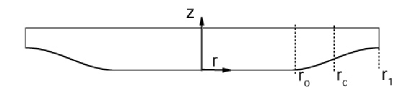
Figure 1: A vertical cross-section of a cylindrical convection layer with a radial ramp in plate separation, $r_{0}$ defines where the ramp begins, $r_{1}$ defines where the ramp ends and $r_{c}$ is where the plate separation corresponds to the critical Rayleigh number. The ramp shown is a cosine ramp given by Eq. (2). For presentation purposes we show a steep ramp with $\delta_{r}=0.25$ (this domain is not used in the simulations).

Experiments using the cosine ramp defined by Eq. (2) have yielded unexpected results for the wavenumber Ahlers et al. (2001); Bajaj et al. (1999). Mean pattern wavenumber measurements (using the Fourier methods discussed in Morris et al. (1993)) yielded $\tilde{k}_{c}=2.97<k_{c}$. Additionally, measurements of the local wavenumber defined at each position in space (method discussed in Egolf et al. (1998)) displayed interesting variation as $\epsilon_{0}$ is increased. For the time independent patterns the bulk region, $r\leq r_{0}$, contains approximately straight parallel rolls. Near threshold, $\epsilon_{0}\lesssim 0.048$, a centered egg-shaped domain of convection rolls with small wavenumber, $k<k_{c}$, extends through the convection cell with the long-axis parallel to the roll axes. A dramatic roll expansion from $k\approx 3.6$ at the edge where the ramp begins to $k\approx 2.6$ in the center of the domain is observed. As $\epsilon_{0}$ increases, the wavenumber field evolves into a domain characterized by large wavenumbers extending through the layer with the long-axis perpendicular to the roll axes (see Fig. 3 of Bajaj et al. (1999)). Similar experiments without a ramp do not exhibit this wavenumber behavior Hu et al. (1993, 1994, 1995).

In the experiments with a radial ramp in plate separation, for $\epsilon_{0}\lesssim 0.03$, time dependent states were found through the repeated formation of defects via an Eckhaus mechanism consistent with the local wavenumbers crossing the Eckhaus stability boundary for an ideal infinite layer of two-dimensional rolls. Also in the ramped experiments, for $\epsilon_{0}\gtrsim 0.18$, defects were formed via a skewed varicose mechanism consistent with the local wavenumber exceeding the skewed varicose stability boundary for an ideal infinite layer of two-dimensional rolls similar to what has been observed in experiments in unramped cylindrical domains with rigid sidewalls Croquette and Williams (1989).

It has been suggested that these features may be the result of the interaction of the convective roll pattern and weak large scale flows Bajaj et al. (1999). The visualization and quantification of these large scale flows is not possible in the current generation of experiments. However, we are able to make these measurements by performing full numerical simulations with a new spectral element code (discussed further in Section III). We utilize the complete knowledge of the flow field together with analytical results valid near threshold to explore this further.

II Large Scale Flows

In this work the terminology large scale flows is used to describe flows that extend over distances larger than that of the convection roll scale. We would like to distinguish between two different large scale flows: large scale counterflow and mean flow.

II.1 Large Scale Counterflow

In the presence of a spatial ramp in plate separation a large scale counterflow is present for all values of the bulk control parameter $\epsilon_{0}$, including $\epsilon_{0}<0$. Warm fluid ascends the ramp eventually reaching the sidewall and is forced to flow back toward the center of the domain over the cold top wall causing it to descend resulting in a large zone of circulation in the vertical plane over the ramp. The magnitude of the large scale counterflow depends upon the specifics of the ramp and is roughly independent of $\epsilon_{0}$ and $\sigma$ Walton (1982). Figure 2 illustrates this with a vertical slice from a three-dimensional numerical simulation where the entire convection layer is subcritical. As shown for this subcritical case the fluid motion of the large scale counterflow generates axisymmetric convection near the base of the ramp which extends a couple of roll widths toward the center of the domain. For the gradual ramp used in experiment the large scale counterflow is small in magnitude and has not been measured.

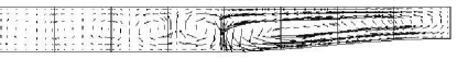
Figure 2: Velocity vectors illustrating the large scale counterflow for a vertical slice of a cylindrical convection layer for subcritical conditions, $\epsilon_{0}=-0.063$. The ramp parameters are $r_{0}=7.66$, $r_{1}=10$, and $\delta_{r}=0.15$. A steep ramp is shown to clearly illustrate the flow. Solid vertical lines indicate the boundaries of the spectral element grid used in the simulation, only a portion of the layer is shown emphasizing the ramped region.

II.2 Mean Flow

In discussing the mean flow it will be convenient to first present the governing heat and fluid equations. The velocity $\vec{u}$, temperature $T$, and pressure $p$, evolve according to the Boussinesq equations,

$${\sigma}^{-1}\left({\partial}_{t}+\vec{u}{\scriptscriptstyle\stackrel{{\scriptstyle\bullet}}{{{}}}}\vec{\nabla}\right)\vec{u} = -\vec{\nabla}p+RT\hat{z}+\nabla^{2}\vec{u},$$ (3)

$$\left({\partial}_{t}+\vec{u}{\scriptscriptstyle\stackrel{{\scriptstyle\bullet}}{{{}}}}\vec{\nabla}\right)T = \nabla^{2}T,$$ (4)

$$\vec{\nabla}{\scriptscriptstyle\stackrel{{\scriptstyle\bullet}}{{{}}}}\vec{u} = 0,$$ (5)

where $\partial_{t}$ indicates time differentiation, and $\hat{z}$ is a unit vector in the vertical direction opposite to gravity. The equations are nondimensionalized in the standard manner using the layer depth $d$, the vertical diffusion time for heat ${\tau}_{v}\equiv d^{2}/\kappa$ where $\kappa$ is the thermal diffusivity, and $\Delta T$ the temperature difference between the top and bottom surfaces, as the length, time, and temperature scales, respectively. The lower and upper surfaces are no-slip and are held at constant temperature. The sidewalls are also no-slip and, unless otherwise noted, are insulating.

The mean flow field, $\vec{U}(x,y)$, is the horizontal velocity integrated over the depth and originates from the Reynolds stress induced by pattern distortions. As illustrated by the fluid equations, Eqs. (3) and (5), it is evident that the pressure is not an independent dynamic variable. The pressure is determined implicitly to enforce incompressibility,

$$\nabla^{2}p=-\sigma^{-1}\vec{\nabla}{\scriptscriptstyle\stackrel{{\scriptstyle\bullet}}{{{}}}}\left[\left(\vec{u}{\scriptscriptstyle\stackrel{{\scriptstyle\bullet}}{{{}}}}\vec{\nabla}\right)\vec{u}\right]+R\partial_{z}T.$$ (6)

Focussing on the nonlinear Reynolds stress term and rewriting the pressure as $p=p_{o}(x,y)+\bar{p}(x,y,z)$ yields,

$$p_{o}(x,y)\sim\sigma^{-1}\int dx^{\prime}dy^{\prime}\ln\left(1/\left|r-r^{\prime}\right|\right)\left<\vec{\nabla}^{\prime}{\scriptscriptstyle\stackrel{{\scriptstyle\bullet}}{{{}}}}\left[\left(\vec{u}{\scriptscriptstyle\stackrel{{\scriptstyle\bullet}}{{{}}}}\vec{\nabla}\right)\vec{u}\right]\right>_{z},$$ (7)

where $\left<\cdot\right>_{z}$ represents an average in the z direction. In Eq. (7) the $\ln(1/|r-r^{\prime}|)$ is not exact, in order to be more precise the finite system Green’s function would be required; however the long range behavior persists. This gives a contribution to the pressure that depends on distant parts of the convection pattern. The Poiseuille-like flow driven by this pressure field subtracts from the Reynolds stress induced flow leading to a divergence free horizontal flow that can be described in terms of a vertical vorticity.

Near threshold an explicit expression for the mean flow is Cross and Newell (1984)

$$\vec{U}(x,y)=-\gamma\vec{k}\vec{\nabla}_{\perp}{\scriptscriptstyle\stackrel{{\scriptstyle\bullet}}{{{}}}}\left(\vec{k}A^{2}\right)-\vec{\nabla}_{\perp}p_{o}(x,y)$$ (8)

where $\gamma$ is a coupling constant given by $\gamma=0.42{\sigma}^{-1}(\sigma+0.34)(\sigma+0.51)^{-1}$, $A^{2}$ is the convection amplitude normalized so that the convective heat flow per unit area relative to the conducted heat flow at $R_{c}$ is $|A|^{2}R/R_{c}$, $p_{o}$ is a slowly varying pressure, see Eq. (7), and $\vec{\nabla}_{\perp}$ is the horizontal gradient operator [see Siggia and Zippelius (1981); Newell et al. (1990) for the complete analysis and more details]. The mean flow is important not because of its strength; under most conditions the magnitude of the mean flow is substantially smaller than the magnitude of the roll flow making it extremely difficult to quantify experimentally. The mean flow is important because it is a nonlocal effect acting over large distances (many roll widths) and changes important general predictions of the phase equation Cross and Newell (1984). The mean flow is driven by roll curvature, roll compression and gradients in the convection amplitude. The resulting mean flow advects the pattern giving an additional slow time dependence. It is important to note, that unlike the long range counterflow, the magnitude of the mean flow vanishes when the convection layer becomes critical, $|\vec{U}|\sim\epsilon_{0}$ for $\epsilon_{0}\ll 1$.

III Numerical Simulation

We have performed full numerical simulations of the governing fluid and heat equations, Eqs. (3)-(5), in a cylindrical geometry with a radial ramp in plate separation using a parallel spectral element algorithm (described in detail elsewhere Fischer (1997), see Paul et al. (2001, submitted March 2002) for related applications).

For discussion purposes it will be convenient to define Cartesian $(x,y)$ and polar $(r,\theta)$ coordinates centered on a mid-depth horizontal slice of a cylindrical convection layer containing a field of straight parallel x-rolls with wavevector $\vec{k}=k_{o}\hat{x}$ as shown in Fig. 3. The x-axis is perpendicular to the roll axes, the y-axis is parallel to the roll axes and $\theta$ measures the angle from the positive x-axis.

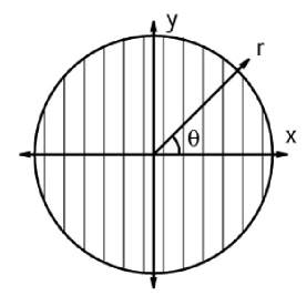
Figure 3: Cartesian $(x,y)$ and polar $(r,\theta)$ coordinates defined on a mid-depth horizontal cross-section of a cylindrical convection layer containing a field of x-rolls described by $\vec{k}=k_{o}\hat{x}$.

We have investigated the results found in experiment by performing simulations on a ramped cylindrical convection layer for a variety of scenarios and initial conditions. Simulations were performed over the range $\epsilon_{0}\lesssim 0.2$ and for simulation times of $t_{f}>\tau_{h}$ where $\tau_{h}\equiv r_{0}^{2}$ is the time required for heat to diffuse horizontally across the bulk region of the layer which has been suggested as the earliest time scale for the flow field to reach equilibrium Cross and Newell (1984).

The mean flow present in the simulation flow fields, $\vec{U}_{s}(x,y)$, is investigated by calculating the depth averaged horizontal velocity,

$$\vec{U}_{s}(x,y)=\int^{1}_{0}\vec{u}_{\perp}dz$$ (9)

where $\vec{u}_{\perp}$ is the horizontal velocity field. Furthermore it will be convenient to work with the vorticity potential, $\zeta$, defined as

$$\nabla^{2}_{\perp}\zeta=-\hat{z}{\scriptscriptstyle\stackrel{{\scriptstyle\bullet}}{{{}}}}\left(\nabla_{\perp}\times\vec{U}_{s}\right)=-\omega_{z}$$ (10)

where $\omega_{z}$ is the vertical vorticity and $\nabla^{2}_{\perp}$ is the horizontal Laplacian.

IV Analytical Development

Near threshold, assuming straight parallel rolls, it is possible to approximately determine $\omega_{z}$ analytically. It will be convenient to start from $\omega_{z}$ given by the vertical component of the curl of Eq. (8),

$${\omega}_{z}=\hat{z}{\scriptscriptstyle\stackrel{{\scriptstyle\bullet}}{{{}}}}\left(\vec{\nabla}_{\perp}\times\vec{U}\right)=-\gamma\hat{z}{\scriptscriptstyle\stackrel{{\scriptstyle\bullet}}{{{}}}}\vec{\nabla}_{\perp}\times\left[\vec{k}\vec{\nabla}_{\perp}{\scriptscriptstyle\stackrel{{\scriptstyle\bullet}}{{{}}}}\left(\vec{k}|A|^{2}\right)\right].$$ (11)

Consider a cylindrical convection layer with a radial ramp in plate separation containing a field of x-rolls given by $\vec{k}=k_{o}\hat{x}$. The amplitude can be represented for large $\epsilon_{0}$, using an adiabatic approximation, as $|A|^{2}=\epsilon(r)/g_{o}$ for $\epsilon>0$ and $|A|^{2}=0$ for $\epsilon(r)<0$, making the amplitude a function of radius only $|A|^{2}=f(r)$. This approximation is good except for the kink at $r_{c}$ where $\epsilon=0$. Inserting $|A|^{2}=f(r)$ into Eq. (11) yields, after some manipulation, the following expression for the vertical vorticity,

$${\omega}_{z}=\frac{\gamma{k_{o}}^{2}}{2}\left[\frac{d^{2}|A|^{2}}{dr^{2}}-\frac{1}{r}\frac{d|A|^{2}}{dr}\right]\sin 2\theta.$$ (12)

To correct for nonadiabaticity and to smooth $|A(r)|^{2}$ near $r_{c}$, the one-dimensional time independent amplitude equation is solved,

$$0=\epsilon(r)A+{{\xi}_{o}}^{2}{\cos}^{2}{\theta}\frac{\partial^{2}A}{\partial r^{2}}-g_{o}|A|^{2}A,$$ (13)

where angular derivatives have been assumed small, ${{\xi}_{o}}^{2}=0.148$, $g_{o}=0.6995-0.0047\sigma^{-1}+0.0083\sigma^{-2}$ and $\epsilon(r)$ is determined by

$$\epsilon(r)=\left\{\begin{array}[]{ll}\epsilon_{0},&\mbox{$r<r_{0}$}\\ \epsilon_{0}(h^{3}-h_{c}^{3})/(1-h_{c}^{3}),&\mbox{$r\geq r_{0}$}\end{array}\right.$$ (14)

where $h_{c}=h(r_{c})$. In Eq. (11) $\omega_{z}$ is dominated by radial derivatives so Eq. (12) is still a good approximation for the case $|A|^{2}=f(r,\theta)$, $d/dr\rightarrow\partial/\partial r$. Due to the angular dependence of the nonadiabaticity $|A|^{2}$ is now $\theta$ dependent which will induce higher angular harmonics in $\omega_{z}$. We will neglect these higher harmonics, assume a $\sin 2\theta$ dependence and approximately evaluate the magnitude using Eqs. (12) and (13) at $\theta=\pi/4$. Equation (13) can be rewritten in a more convenient form as,

$$0=\frac{\epsilon(\bar{r})}{\epsilon_{0}}\bar{A}+\frac{\partial^{2}\bar{A}}{\partial\bar{r}^{2}}-\bar{A}^{3}$$ (15)

where $r=\left({{\epsilon}_{0}}^{-1/2}{\xi}_{o}\cos\theta\right)\bar{r}$ and $A={(\epsilon_{0}/g_{o})}^{1/2}\bar{A}$ Cross and Newell (1984) (since the amplitude goes to zero it can be shown that $A$ is now a real quantity Cross et al. (1983)). Equation (15) is solved numerically using the boundary conditions $\partial_{\bar{r}}\bar{A}=0$ at $\bar{r}=0$, and $\bar{A}=0$ at $\bar{r}={\bar{r}}_{1}$.

These analytical results are now used to investigate the vertical vorticity generation in a large radially ramped cylindrical convection layer. We start by looking at the configuration used in the recent experiments with input parameters: $r_{0}=42.29$, $r_{1}=101.33$, ${\delta}_{r}=0.036$ and $\sigma=0.87$.

When ${\epsilon_{0}}^{1/2}{\xi_{o}}^{-1}(r_{c}-r_{0})\lesssim 1$ the amplitude $A^{2}(r)$ is unable to adiabatically follow the ramp, this nonadiabaticity results in a considerable deviation from $\epsilon(r)/g_{o}$ as shown in Fig. 4. However, when ${\epsilon_{0}}^{1/2}{\xi_{o}}^{-1}(r_{c}-r_{0})\gg 1$ the amplitude $A^{2}(r)$ follows $\epsilon(r)/g_{o}$ adiabatically almost over the entire ramp except for the small kink at $r_{c}$ as shown in Fig. 5. The structure of $\omega_{z}$ depends upon this adiabaticity and is shown for various values of $\epsilon_{0}$ in Fig. 6 where the $\sin 2\theta$ dependence has been removed by choosing $\theta=\pi/4$.

If the $\theta$ dependence is included it is evident from Fig. 6 that the vertical vorticity has a quadrupole angular structure for small $\epsilon_{0}$, i.e. four lobes of alternating positive and negative vorticity with one lobe per quadrant, and makes a transition to an octupole angular dependence for larger $\epsilon_{0}$, octupole in the sense of an inner, $r\lesssim r_{c}$, and outer, $r\gtrsim r_{c}$, quadrupole. In addition, since $\partial r_{c}/\partial\epsilon_{0}>0$ there is a radial shift of the vorticity curves as $\epsilon_{0}$ is increased.

In all cases the amplitude $A^{2}(r)$ decreases monotonically with $r$ and as a result $-r^{-1}~{}d|A|^{2}/dr\geq 0$ thus generating only positive vorticity. However, the term $d^{2}|A|^{2}/dr^{2}$ can be of either sign and is responsible for the quadrupole and octupole angular structure in $\omega_{z}$.

Figure 4: The solution of Eq. (15) plotted as $A^{2}(r)$ for $r_{0}=42.29$, $r_{c}=47.56$, $r_{1}=101.33$, $\delta_{r}=0.036$, $\sigma=0.87$ and $\epsilon_{0}=4.20\times 10^{-3}$. Also shown for comparison is $\epsilon(r)/g_{o}$.

Figure 5: The solution of Eq. (15) plotted as $A^{2}(r)$ for $r_{0}=42.29$, $r_{c}=80.05$, $r_{1}=101.33$, $\delta_{r}=0.036$, $\sigma=0.87$ and $\epsilon_{0}=0.17$. Also shown for comparison is $\epsilon(r)/g_{o}$.

Figure 6: Dependence of the radial variation of $\omega_{z}=\omega_{z}(r)$ with $\epsilon_{0}$ as determined analytically from Eqs. (12) and (15) illustrating the evolution from a mean flow with a quadrupole dependence to an octupole dependence as $\epsilon_{0}$ increases. Shown explicitly are $\omega_{z}$ curves for $\epsilon_{0}=7.2\times 10^{-3}$, $4.2\times 10^{-3}$, and $1.3\times 10^{-3}$ with the parameters $r_{0}=42.29$, $r_{1}=101.33$, $\delta_{r}=0.036$ and $\sigma=0.87$ labelled (a)-(c), respectively.

As $\epsilon_{0}$ approaches zero the nonadiabaticity of $A^{2}(r)$ increases until $A^{2}(r)$ exhibits a quadratic fall-off with $r$ for $r\ll r_{0}$ resulting in $\omega_{z}(r)\geq 0$ for all $r$.

The mean flow generated by these vorticity distributions is determined by solving Eq. (11) with the boundary condition $\zeta(r_{1})=0$. The vorticity potential is related to the mean flow in polar coordinates by $(U_{r},U_{\theta})=(r^{-1}\partial_{\theta}\zeta,-\partial_{r}\zeta)$. The vorticity potential is expanded radially in second order Bessel functions while maintaining the $\sin 2\theta$ angular dependence. Of particular interest is the mean flow perpendicular to the convection rolls, $U_{r}(\theta=0)$ or equivalently $U_{x}(y=0)$, which is shown in Fig. 7.

Figure 7: Variation of the mean flow, $U_{x}(y=0)$ with $\epsilon_{0}$ as determined from Eq. (10). Shown explicitly are curves for $\epsilon_{0}=7.2\times 10^{-3}$, $4.2\times 10^{-3}$, and $1.3\times 10^{-3}$ labelled (a)-(c), respectively with the parameters $r_{0}=42.29$, $r_{1}=101.33$, $\delta_{r}=0.036$ and $\sigma=0.87$.

As expected, regions of negative and positive vorticity yield corresponding negative and positive values of the mean flow. As $\epsilon_{0}$ vanishes $U\geq 0$ for all $r$ providing a mechanism for roll expansion in the bulk. For larger $\epsilon_{0}$ the mean flow becomes larger in magnitude and increasingly negative for $r\leq r_{0}$ providing a mechanism for roll compression.

To make the connection between mean flow and wavenumber quantitative it is noted that the wavenumber variation resulting from a mean flow across a field on x-rolls can be determined from the one-dimensional phase equation,

$$U\partial_{x}\phi=D_{\parallel}\partial_{xx}\phi$$ (16)

where the wavenumber is the gradient of the phase, $k=\partial_{x}\phi$, $D_{\parallel}=\xi_{o}^{2}\tau_{o}^{-1}$, and $\tau_{o}^{-1}=19.65\sigma(\sigma+0.5117)^{-1}$ Cross and Hohenberg (1993). Assuming that for $\epsilon_{0}\ll 1$ the wavenumber is approximately $k\approx k_{c}$ everywhere and that the rolls are exposed to a constant mean flow the wavenumber change over the bulk can be expressed as

$$\Delta k=k(r_{0})-k(r=0)=Uk_{c}D_{\parallel}^{-1}r_{0}.$$ (17)

For example, for curve (c) in Fig. 7 the maximum value of the mean flow is $U=4.92\times 10^{-5}$ which yields a small roll expansion of $\Delta k=0.0035$. If the mean flow were solely responsible for the dramatic roll expansion seen in experiment of $\Delta k\approx 1.0$ ($\epsilon_{0}=0.012$ see Fig. 3(a) of Bajaj et al. (1999)) a mean flow of $U\approx 0.014$ would be required, which is not found in the analytic results.

V Discussion

The large scale flows discussed in Section II cannot be measured in current experiments placing us in a unique position to use the complete flow field information from our full numerical simulations of Eqs. (3)-(5) together with the analytical results of Section IV to investigate how the mean flow and the large scale counterflow induce wavenumber distortions and the variation of this distortion with Rayleigh number.

It is computationally expensive to perform full three-dimensional numerical simulations for the very large system used in experiment. We have, however, performed a variety of simulations for radially ramped cylindrical convection layers. The full three-dimensional simulations are of smaller spatial extent with the precise ramp defined by Eq. (2) and the specific input parameters: $r_{0}=11.31$, $r_{1}=20$, $\delta_{r}=0.036$, and $\sigma=0.87$. Two-dimensional simulations of a vertical slice of a three-dimensional domain (see Fig. 1) were also performed for both the large experimental configuration and the smaller computational domain just described. Three-dimensional simulations were also conducted without a large scale counterflow by a specific choice of ramp parameters that will be discussed below.

Initially we consider prescribed x-roll initial conditions given by $\vec{k}=k_{c}\hat{x}$. Other initial conditions such as random thermal perturbations or initial x-rolls of varying wavenumbers were also investigated and found not to affect the final pattern wavenumber or any of the conclusions drawn. Simulations were performed for $\epsilon_{0}=0.025$, 0.054, 0.113, and 0.171. Figure 8 compares the wavenumbers found in these simulations with recent experiments and will be discussed in detail below.

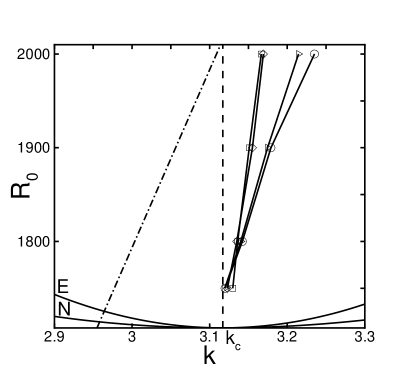
Figure 8: Comparison of the mean wavenumber variation as a function of the bulk Rayleigh number (i.e. for $r\leq r_{0}$), $R_{0}$, between simulation (solid lines with symbols) and experiment (dashed-dotted line) Bajaj et al. (1999). Unless otherwise noted $r_{0}=11.31$, $r_{1}=20$, $\delta_{r}=0.036$, and $\sigma=0.87$. The symbols represent: $(\circ)$ three-dimensional simulations, ($\square$) two-dimensional simulations, ($\triangleright$) three-dimensional simulations for a specific ramp construction without a large scale counterflow, and ($\diamond$) two-dimensional simulations with $r_{0}=42.29$, and $r_{1}=101.33$. Dark solid lines denote the approximate location of the neutral (N) and Eckhaus (E) stability boundaries for an ideal infinite layer of parallel rolls.

The final patterns in the simulations maintain the x-roll configuration imposed by the initial conditions. Figure 9 displays the final pattern observed for three-dimensional simulations with $\epsilon_{0}=0.025$ in panel (a) and $\epsilon_{0}=0.171$ in panel (b). Figure 9a illustrates that near threshold the convection rolls exhibit very little curvature indicating that the assumption of straight parallel x-rolls in Section IV is valid. There is more roll curvature apparent in Fig. 9b as would be expected for larger $\epsilon_{0}$. Figure 9 also illustrates the decreasing size of the subcritical region as the supercriticality of the bulk increases. All simulations settled to a time independent state.

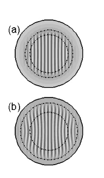
Figure 9: Final convection patterns for $\epsilon_{0}=0.025$ and $0.17$ are shown in panels (a) and (b), respectively. Shaded contours of the thermal perturbation are shown with dark regions representing cool descending fluid and light regions warm ascending fluid. The inner dotted circle indicates where the ramp begins, $r_{0}$, and the outer dotted circle indicates where the convection layer becomes critical, $r_{c}$. Simulation parameters, $r_{0}=11.31$, $r_{1}=20$, $\delta_{r}=0.036$, $\sigma=0.87$.

It is illustrative to compare the analytical results of Section IV with the results of simulation. Figure 10a displays $A^{2}(r)$ for the case $\epsilon_{0}=0.025$, as determined by Eq. (15). A significant nonadiabaticity is present for this case as shown by the deviation of $A^{2}(r)$ from $\epsilon(r)/g_{o}$. For the ramped domain used in simulation the distance $r_{c}(\epsilon_{0})-r_{0}$ is smaller than in the larger domain with a more shallow ramp used in experiment. This results in the presence of more nonadiabaticity in the simulations when compared to experimental results at the same control parameter. This is beneficial because this allows the exploration of highly nonadiabatic situations without having to perform the task of simulating near the convective threshold, which becomes computationally difficult because of the diverging time scales.

A comparison between theory and simulation of the vertical vorticity and the resulting mean flow is shown in Fig. 10b and c. The theoretical predictions are based on the amplitude variation caused when straight parallel convection rolls encounter a radial ramp in plate separation as discussed in Section IV. For both the vertical vorticity and the mean flow the comparison is made in the absence of any adjustable parameters. For the vertical vorticity calculated in simulation an angular average, weighted by $\sin 2\theta$, is used for the comparison. The agreement between theory and simulation is quite good. This illustrates quantitatively that the major source of vertical vorticity and mean flow is indeed the variation in the convective amplitude caused by the radial ramp in plate separation. Over the bulk of the domain the mean flow is negative and very small in magnitude with a maximum value of $U_{x}(y=0)=-7.0\times 10^{-4}$ and by Eq. (17) the wavenumber variation would be extremely small in agreement with the near constant bulk wavenumbers found in simulation.

Figure 10: Panel (a) shows the solution of Eq. (15) plotted as $A^{2}(r)$, shown for comparison is $\epsilon(r)/g_{o}$. Panel (b) compares the vertical vorticity found analytically from Eq. (15) with an angular average, weighted by $\sin 2\theta$, of the vertical vorticity from simulation. Panel (c) compares the mean flow found analytically from Eq. (10) with the mean flow from simulation flowing along the x-axis at $y=0$. Parameters are $r_{0}=11.31$, $r_{c}=13.20$, $r_{1}=20.0$, $\delta_{r}=0.036$, $\sigma=0.87$ and $\epsilon_{0}=0.025$.

A similar comparison between theory and simulation is made in Fig. 11 for $\epsilon_{0}=0.171$. As shown in Fig. 11a $A^{2}(r)$ is much more able to follow the ramp, $\epsilon(r)/g_{o}$, and exhibits very little nonadiabaticity except for the kink near $r_{c}$. This results in a much stronger negative vertical vorticity in the bulk which in turn yields a larger negative mean flow as shown if Fig. 11b and c. The agreement between theory and simulation for the vertical vorticity is still quite good. The discrepancy in the mean flow comparison may be due to the fact that as $\epsilon_{0}$ increases other mean flow sources such as roll curvature, see Fig. 9b, become important.

Figure 11: Panel (a) shows the solution of Eq. (15) plotted as $A^{2}(r)$, shown for comparison is $\epsilon(r)/g_{o}$. Panel b compares the vertical vorticity found analytically from Eq. (15) with an angular average, weighted by $\sin 2\theta$, of the vertical vorticity from simulation. Panel (c) compares the mean flow found analytically from Eq. (10) with the mean flow from simulation flowing along the x-axis at $y=0$. Parameters are $r_{0}=11.31$, $r_{c}=13.20$, $r_{1}=20.0$, $\delta_{r}=0.036$, $\sigma=0.87$ and $\epsilon_{0}=0.171$.

Figure 12 illustrates the octupole structure in the vorticity potential in panel (a) and the roll compression occurring in the bulk by plotting contours of the local wavenumber in panel (b) for $\epsilon_{0}=0.171$. As illustrated in panel (a) the mean flow has significant structure over the ramped region as well as extending into the subcritical region of the layer, $r>r_{c}$. It has also been suggested that the mean flow extends into a subcritical region in related experiments implementing “finned” boundaries Pocheau and Daviaud (1997).

The vorticity potential displays an octupole structure containing a pair of counter-rotating vortices in each quadrant. The inner quadrupole is localized around $r_{0}$ where gradients in the amplitude of convection occur as the ramp in plate separation begins. The direction of rotation of the inner quadrupole causes a focussing of the mean flow into the bulk region of the domain and is responsible for the larger wavenumbers found as $\epsilon_{0}$ is increased as shown by the ($\circ$) curve in Fig. 8.

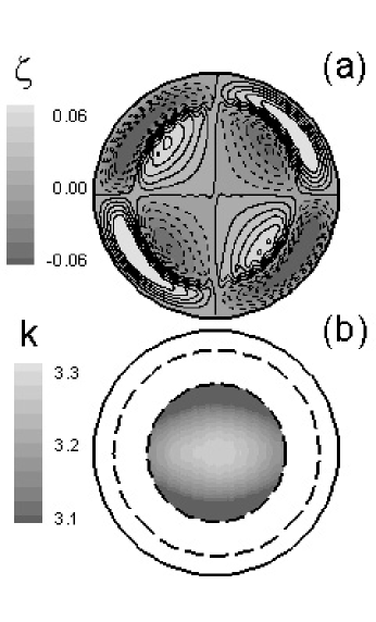
Figure 12: Contours of the vorticity potential $\zeta$, panel (a), (light indicates counterclockwise rotation drawn with solid contours and dark indicates clockwise rotation drawn with dashed contours) and the corresponding local wavenumber distribution, $k$, panel (b). The magnitude of the mean flow is approximately $2\%$ of the magnitude of the velocity field, $|\vec{U}_{s}|/|\vec{u}|\approx 0.02$. Local wavenumber distributions are shown only in the bulk, $r\leq r_{0}$. The inner dotted circle indicates where the ramp begins, $r_{0}$, and the outer dotted circle indicates where the convection layer becomes critical, $r_{c}$. Simulation parameters, $r_{0}=11.31$, $r_{1}=20$, $\delta_{r}=0.036$, $\sigma=0.87$ and $\epsilon_{0}=0.171$ ($R_{0}=2000$).

To make the connection between mean flow and wavenumber quantitative Eq. (16) is applied to the simulation results in the form,

$$U=D_{\parallel}k_{c}^{-1}\partial_{x}k.$$ (18)

Figure 13a illustrates the wavenumber variation, $k(r)$ for $r\leq r_{0}$, found in simulation by simply measuring the distance between roll boundaries and makes evident the roll compression, $k(r=0)>k(r_{0})$. Figure 13b compares the mean flow calculated from simulation with the predicted value of the mean flow required to produce the wavenumber variation shown in Fig. 13a using Eq. (18). The agreement is good and the discrepancy near $r_{0}$, which is contained within one roll wavelength from where the ramp begins, is expected because the influence of the ramp was not included in Eq. (16). This illustrates quantitatively that the mean flow compresses the rolls in the bulk of the domain.

Figure 13: Panel (a), the variation in the local wavenumber along the positive x-axis, or equivalently $k(r)$ at $\theta=0$. Panel (b), a comparison of the mean flow from simulation (solid line) with the predicted value calculated from Eq. (16) using the wavenumber variation from panel (a). Simulation parameters, $r_{0}=11.31$, $r_{1}=20$, $\delta_{r}=0.036$, $\sigma=0.87$ and $\epsilon_{0}=0.171$ ($R_{0}=2000$).

As mentioned earlier, the mean flow vanishes as $\epsilon_{0}$ approaches critical whereas the large scale counterflow is present for all $\epsilon_{0}$ and therefore could play a role near threshold in the determination of the final convection pattern. In order to gain further insight into this possibility a radial ramp was constructed that did not drive a large scale counterflow. This was accomplished by setting the temperature of the ramped surface, $T_{b}(r)$, to the value of the linear conduction profile at that height, $T_{b}(r)=h(r)$. This ramp, therefore, does not bend the isotherms which is the source of the large scale counterflow. The wavenumber variation for these simulations, see curve labelled with ($\triangleright$) in Fig. 8, does not differ strongly from the simulations with a ramp producing large scale counterflow, see the curve labelled with ($\circ$). The similarity in wavenumber results is strongest for small $\epsilon_{0}$ suggesting that the large scale counterflow is not responsible for the shift of the critical wavenumber to smaller values as seen in experiment.

To study the large scale counterflow further two-dimensional simulations were also performed, corresponding to a vertical slice of the domain considered thus far, and in addition to a more spatially extended domain as used in experiment. In two dimensions the mean flow is absent however the large scale counterflow persists. As shown by the ($\diamond$) and ($\square$) curves in Fig. 8 the wavenumbers measured in the two-dimensional simulations are not compressed to the same extent as $\epsilon_{0}$ increases as in the three-dimensional simulations with both mean flow and large scale counterflow present. As expected, the wavenumbers found in the two-dimensional simulations are also independent of aspect ratio. Additionally, for small $\epsilon_{0}$ the wavenumber found in simulation does not deviate markedly from its critical value suggesting that the large scale counterflow is not responsible for the wavenumber shift observed in experiment near threshold regardless of the spatial extent of the domain.

We also investigated the possibility that the vertical large scale counterflow could bifurcate into a horizontal flow similar to the mean flow in the presence of a slight spatial asymmetry. This was accomplished by giving the ramped domain used in the full three-dimensional simulations an eccentricity of $e\approx 0.8$ for a variety of ramps $0.036\leq\delta_{r}\leq 0.25$ and simulating over a range of subcritical and supercritical conditions. For all of the scenarios tested the large scale counterflow remained vertical and did not undergo any significant changes.

Lastly, the possibility of wavenumber pinning was studied by varying the aspect ratio in increments of less than half of a roll width for both the two- and three-dimensional domains. In all of the scenarios tested the final pattern wavenumbers were not appreciably affected by these small changes in aspect ratio.

VI Conclusion

We have analytically and numerically investigated pattern formation in a cylindrical convection layer with a radial ramp in plate separation. In particular, we have studied quantitatively the effects of two large scale flows; large scale counterflow and mean flow. These large scale flows are important theoretically yet are extremely difficult to measure experimentally.

Our results suggest that the mean flow plays an important role in the observed pattern wavenumber and is generated in a novel way, by the spatial variation of $|A|^{2}$ driven by the variation of $\epsilon$ rather than the more usual variations in roll curvature and wavenumber. The mean flow sources are quantified analytically and agreement is found with numerical results. The geometric structure and magnitude of the mean flow is used to explain quantitatively the wavenumber variation found in the simulations.

The large scale counterflow is investigated numerically and our results indicate a small roll compression effect away from threshold. In particular, although the large scale counterflow is present at and near threshold it does not appear responsible for the dramatic wavenumber shift to values less than critical as seen in experiment.

Although it is too expensive computationally to simulate the very large systems used in the experiments we can use our quantitative understanding of the ramp-generated mean flow, validated by the simulations at smaller aspect ratio, to extrapolate our results to these larger systems. Furthermore our two-dimensional simulations in sizes equal to the experimental ones allow us to estimate the effect of the large scale counterflow on the wavenumber distribution. Despite these exhaustive efforts, we are unable to reproduce the large shift to smaller wavenumbers observed near threshold in the experiments, and the physical origin of these results remains a mystery.

References

- Cross and Hohenberg (1993) M. C. Cross and P. C. Hohenberg, Rev. of Mod. Phys. 65(3 II), 851 (1993).
- Cross et al. (1986) M. C. Cross, G. Tesauro, and H. S. Greenside, Physica D 23, 12 (1986).
- Catton (1988) I. Catton, J. Heat Trans. 110, 1154 (1988).
- Getling (1998) A. V. Getling, Rayleigh-Bénard Convection (World Scientific, Singapore, 1998).
- Eagles (1980) P. M. Eagles, Proc. R. Soc. Lond. A 371, 359 (1980).
- Kramer et al. (1982) L. Kramer, E. Ben-Jacob, H. Brand, and M. C. Cross, Phys. Rev. Lett. 49(26), 1891 (1982).
- Kramer and Riecke (1985) L. Kramer and H. Riecke, Z. Phys. B 59, 245 (1985).
- Buell and Catton (1986) J. C. Buell and I. Catton, J. Fluid Mech. 171, 477 (1986).
- Bajaj et al. (1999) K. M. S. Bajaj, N. Mukolobwiez, N. Currier, and G. Ahlers, Phys. Rev. Lett. 83(25), 5282 (1999).
- Pomeau and Zaleski (1983) Y. Pomeau and S. Zaleski, J. Phys. Lett. 44, L135 (1983).
- Ahlers et al. (2001) G. Ahlers, K. M. S. Bajaj, N. Mukolobwicz, and J. Oh, unpublished (2001).
- Morris et al. (1993) S. W. Morris, E. Bodenschatz, D. S. Cannell, and G. Ahlers, Phys. Rev. Lett. 71(13), 2026 (1993).
- Egolf et al. (1998) D. A. Egolf, I. V. Melnikov, and E. Bodenschatz, Phys. Rev. Lett. 80(15), 3228 (1998).
- Hu et al. (1993) Y. Hu, R. E. Ecke, and G. Ahlers, Phys. Rev. E 48(6), 4399 (1993).
- Hu et al. (1994) Y. Hu, R. E. Ecke, and G. Ahlers, Phys. Rev. Lett. 72(14), 2191 (1994).
- Hu et al. (1995) Y. Hu, R. Ecke, and G. Ahlers, Phys. Rev. E 51, 3263 (1995).
- Croquette and Williams (1989) V. Croquette and H. Williams, Physica D 37, 300 (1989).
- Walton (1982) I. C. Walton, Stud. Appl. Maths. 67, 199 (1982).
- Cross and Newell (1984) M. C. Cross and A. C. Newell, Physica D 10, 299 (1984).
- Newell et al. (1990) A. C. Newell, T. Passot, and M. Souli, J. Fluid Mech. 220, 187 (1990).
- Siggia and Zippelius (1981) E. D. Siggia and A. Zippelius, Phys. Rev. Lett. 47, 835 (1981).
- Fischer (1997) P. F. Fischer, J. Comp. Phys. 133, 84 (1997).
- Paul et al. (2001) M. R. Paul, M. C. Cross, P. F. Fischer, and H. S. Greenside, Phys. Rev. Lett. 87(15), 154501 (2001).
- Paul et al. (submitted March 2002) M. R. Paul, K.-H. Chiam, M. C. Cross, P. F. Fischer, and H. S. Greenside, Physica D (submitted March 2002).
- Cross et al. (1983) M. C. Cross, P. G. Daniels, P. C. Hohenberg, and E. D. Siggia, J. Fluid. Mech. 127, 155 (1983).
- Pocheau and Daviaud (1997) A. Pocheau and F. Daviaud, Phys. Rev. E 55(1), 353 (1997).