Experimental Test of a Trace Formula for a Chaotic Three Dimensional Microwave Cavity

Abstract

We have measured resonance spectra in a superconducting microwave cavity with the shape of a three-dimensional generalized Bunimovich stadium billiard and analyzed their spectral fluctuation properties. The experimental length spectrum exhibits contributions from periodic orbits of non-generic modes and from unstable periodic orbits of the underlying classical system. It is well reproduced by our theoretical calculations based on the trace formula derived by Balian and Duplantier for chaotic electromagnetic cavities.

In the last few decades, billiard systems have provided a most appropriate model for the understanding and discussion of classical chaotic Hamiltonian systems [1] and their quantum counterparts [2]. In two dimensions the Schrödinger equation for quantum billiards coincides with the Helmholtz equation for microwave cavities of corresponding shape. This correspondence is the basis for experimental studies of quantum manifestations of classical chaos. Early experiments focused on spectral fluctuation properties in chaotic billiards [3, 4]. About 30 years ago Gutzwiller established a direct relationship between the oscillating part of the density of states and the properties of the classical periodic orbits by means of a trace formula [5]. Gutzwiller’s trace formula and its extension to systems with mixed classical dynamics [6] were verified experimentally using flat microwave cavities [4, 7]. Three-dimensional chaotic billiard systems have been scarcely studied theoretically [8, 9]. There is no analogy between quantum billiards and electromagnetic cavities in three dimensions. Still, the latter are of great interest for the study of wave dynamical phenomena in chaotic systems. Spectral properties of the vectorial Helmholtz equation have recently been studied theoretically for integrable systems [10] and experimentally for mixed and chaotic systems [11, 12, 13].

We present the first experimental test of the trace formula derived by Balian and Duplantier [14] for chaotic electromagnetic resonators. The main difficulty to overcome consists in the construction of a microwave resonator that is completely chaotic while permitting only a few non-generic modes. We meet these requirements by using a superconducting resonator with the shape of a desymmetrized three-dimensional stadium billiard [15]. Figure 1 shows that this billiard consists of two quarter cylinders with radii $r_{1}$ and $r_{2}$, resp. The electromagnetic resonator has dimensions $r_{1}=200.0~{}{\rm mm},\ r_{2}=141.4~{}{\rm mm}$ and is made of niobium which becomes superconducting at temperatures below 9.2 K. This tremendously increases the resolution of the measured spectra due to a quality factor of up to $10^{7}$ compared to $10^{3}$ in normal conducting resonators. The measurements were performed at a temperature of 4.2 K for frequencies $f$ up to $20$ GHz. We show a typical spectrum in Fig. 2. The evaluation of four reflection and six transmission spectra yielded 18764 resonances. According to Weyl‘s formula [14, 16] for electromagnetic cavities the smooth part of the integrated resonance density, ${N_{\rm smooth}(f)}$, is a polynomial of third order in the frequency, where, in contrast to the corresponding quantum case, the quadratic term is absent. Its coefficients have been obtained by a fit to ${N(f)}$. The fluctuating part $N_{\rm fluc}(f)$ is shown in Fig. 3; it still displays smooth oscillations, which are due to the non-generic periodic orbits. Our cavity (see Fig. 1) exhibits two types of non-generic orbits. First, there are two families of three-dimensional, marginally stable “bouncing ball” orbits with length $2r_{1}$ and $2r_{2}$ that evolve parallel to the axis of the two cylinders. Second, there are trajectories inside the plane $z=0$ that are linearly stable with respect to deviations parallel to this plane and unstable with respect to perpendicular deviations. While both types of orbits are of measure zero, they generate smooth oscillations in the staircase function and yield dominant peaks in the length spectrum, i.e. the absolute value of the Fourier transform of the fluctuating part of the $k$-dependent density of states, where $k=2\pi f/c_{0}$ is the wave number, $c_{0}$ denotes the speed of light. Such effects of non-generic periodic orbits have been found in various types of billiards [4, 13, 17]. The experimental length spectrum is shown in the top of Fig. 4. To obtain an analytical expression for the staircase function of the non-generic modes we combine the semiclassical method of Ref.[12] with the adiabatic method of Ref.[18]. The quantum adiabatic method [18] has been applied to the calculation of bouncing ball modes in the two-dimensional stadium billiard. This method corresponds to a Born-Oppenheimer approximation, where the fast coordinate is parallel to the classical motion corresponding to the bouncing ball orbits, while the slow variable is transversal to it. Accordingly, we assume that the modes in the $x-$ and $y-$directions are adiabatically decoupled from the modes in the $z$-direction and quantize the rectangle with side lengths $l_{x}$ and $l_{y}$. Then, the $x-$ and $y-$component of the wave vector $\vec{k}_{\rm ng}$ of the non-generic modes are given as $k_{x}={\pi\mu/l_{x}}$ and $k_{y}={\pi\nu/l_{y}}$ for integers $\mu$ and $\nu$, where, according to the geometry of our billiard the $z$-dependence of the lengths $l_{x}$ and $l_{y}$ is

$\displaystyle\begin{array}[]{lllrl}l_{x}(z)=r_{1},&l_{y}(z)=\sqrt{r_{2}^{2}-z^{2}}&~{}~{}\mbox{for}&0&\leq z\leq r_{2}\\ l_{y}(z)=r_{2},&l_{x}(z)=\sqrt{r_{1}^{2}-z^{2}}&~{}~{}\mbox{for}&-r_{1}&\leq z<0.\end{array}$

Combining this adiabatic method with the approach of ref. [12] we express the staircase function $N_{\rm ng}(k)$ for the non-generic modes (ng) as $N_{\rm ng}(k)={\rm Tr}\Theta(k^{2}-k_{\rm ng}^{2})$, where the trace is over the wave vector $\vec{k}_{\rm ng}$ of the non-generic modes

$$N_{\rm ng}(k)=\sum_{\mu,\nu}\int{dzdk_{z}\over 2\pi}\,\Theta\left(k^{2}-k_{x}^{2}-k_{y}^{2}-k_{z}^{2}\right).$$ (1)

Note that the integration over $z$ is restricted to the interval $[-r_{1},r_{2}]$ while the $k_{z}$-integration is unrestricted. The integers $\mu$ and $\nu$ label the modes in $x-$ and $y-$directions, resp. Dirichlet ($\mu,\nu>0$) or von Neumann ($\mu,\nu\geq 0$) boundary conditions correspond to the magnetic and electric non-generic modes, resp.

For the electromagnetic cavity under consideration, the non-generic magnetic and electric modes decouple. Thus, the non-generic contribution to the staircase function is given by the sum of the quantum mechanical expression for Dirichlet and von Neumann boundary conditions. Figure 3 shows that the smooth oscillations of the fluctuating part of the experimental staircase function are well described by our expression. Thus, the adiabatic method yields a very good approximation for the contributions of the non-generic modes to the staircase function. In order to study the local fluctuation properties in the resonance spectrum, we rescaled the resonances to unit mean spacing and subtracted the non-generic contributions from the spectrum. For a time-reversal invariant, classically chaotic system the local fluctuation properties are expected to coincide with those of random matrices from the Gaussian orthogonal ensemble (GOE) [19, 20]. We however find notable deviations and attribute them to a partial decoupling between electric and magnetic modes which is prominent at low frequencies. Indeed, our spectral statistics are in very good agreement with that obtained for random matrices $\hat{H}$ from an ensemble, that models two coupled, chaotic systems [21, 22, 23],

$$\hat{H}=\left(\matrix{\hat{H}_{e}&\sqrt{\lambda}Dv_{ij}\cr\sqrt{\lambda}Dv_{ji}&\hat{H}_{m}\cr}\right).$$ (2)

Here, $\hat{H}_{e}$ and $\hat{H}_{m}$ are matrices from the GOE with dimensions $N_{e}$ and $N_{m}$, resp. The coupling matrix elements $v_{ij}$ are Gaussian random variables with zero mean and unit variance, $D$ is the mean level spacing, and $\lambda$ is the coupling strength. The random matrix model interpolates between two uncoupled GOE-systems at $\lambda=0$ and one GOE at $\lambda=1$. We obtain the best agreement between our experimental level statistics and that of random matrices $\hat{H}$ as defined in Eq. (2) when we treat $\lambda$ as a fitting parameter and set $N_{e}$ ($N_{m}$) equal to the number of eigenvalues of the scalar Helmholtz equation with von Neumann (Dirichlet) conditions on the boundary of the billiard. This suggests an interpretation of model (2) in terms of electric and magnetic modes that are coupled with strength $\lambda$. Figure 5 shows the level-spacing distribution and the $\Delta_{3}$-statistics for a frequency range of 5-10 GHz ($\lambda=0.352$) and 18-18.5 GHz ($\lambda=0.658$). The level-spacing distributions agree well with the GOE and with those of the model defined by Equation (2). The $\Delta_{3}$-statistics coincides with that for the random matrix model (2) but differs from the GOE. Note, however, that the GOE is approached with increasing frequency, (2-5 GHz: $\lambda=0.07$, 11.5-13 GHz: $\lambda=0.546$, 15-17 GHz: $\lambda=0.633$). We furthermore found that $2\pi\lambda=\Gamma/D$, where $1/D$ ist the level density, while $\Gamma$ shows only a weak dependence on frequency for the frequency range from 0 to 20 GHz. This is similar to a behavior that was observed in studies of isospin mixing in nuclei [24]. The partial decoupling of electric and magnetic modes at low frequencies was not observed in the three-dimensional Sinai billiard [13] and seems to be due to the particular geometry of the three-dimensional generalized stadium billiard. Its desymmetrized version (see Fig. 1) corresponds to two quarter cylinders, which are rotated by $\pi/2$ with respect to each other. The electric and the magnetic modes are completely decoupled in each of these quarter cylinders [10].

Let us finally turn to a semiclassical analysis of the experimental spectrum. According to [14] the generic contribution to the fluctuating part of the density of states is semiclassically given by the periodic orbit sum, i.e. the trace formula

$$\rho_{\rm fluc}(k)=\sum_{p}{2\cos{(\phi_{p})}L_{p}/\pi\over|{\rm det}(1-M_{p})|^{1/2}}\cos{\left(kL_{p}-{\pi\over 2}\mu_{p}\right)}.$$ (3)

The factor $2\cos{\phi_{p}}$ stems from the polarization and is thus due to the vectorial character of the underlying wave equation. It vanishes for orbits with an odd number of reflections. The remaining quantities in Eq. (3) are identical to those appearing in Gutzwiller’s trace formula [5]. We numerically determined the first 381 periodic orbits, their lengths $L_{p}$ up to about 1.5 m, and their stability matrices $M_{p}$ by two different methods. Based on an ansatz for a symbolic code (see, e.g., Chap. 8 in ref. [3]) we determined all orbits in the full (not the desymmetrized) three-dimensional stadium billiard for up to eight reflections off the boundary. For more reflections the numerical evaluations become too time consuming. The resulting list of periodic orbits was checked for completeness and enlarged by a numerical search of fixed points in the Poincaré surface of section $(z=0,p_{z}>0)$. The latter method is blind to some whispering gallery modes. As in the two-dimensional stadium billiard our device exhibits infinitely many whispering gallery modes. The shortest of these orbits propagate along the curved edges of the billiard and have lengths $2r_{1}+\pi r_{2}\approx 0.843$m, $2r_{2}+\pi r_{1}\approx 0.910$m and $\pi(r_{1}+r_{2})\approx 1.07$m. There are no significant peaks associated with these lengths (see Fig. 4, top). Similar cancellation effects have been observed in the two-dimensional stadium billiard [25]. For the computation of the Maslov indices $\mu_{p}$ we followed [26]. Figure 4 shows a comparison between the experimentally obtained length spectrum, the length spectrum for the sum of non-generic orbits [Eq. (1)] plus unstable periodic orbits [Eq. (3)], and the length spectrum of the unstable periodic orbits alone. Diamonds mark those peaks of the non-generic contributions, that cannot be assigned to bouncing ball modes but to orbits in the plane $z=0$. Evidently, the theoretical reconstruction describes the experiment rather well. One peculiarity are peaks that appear at about $l\approx 0.77~{}$m and $l\approx 0.97~{}$m. While we could not find corresponding orbits inside the billiard, there are two orbits in the boundary plane $y=0$, whose lengths and stability amplitudes exactly match those peaks. Peaks at lengths below $l=0.28~{}$m, which corresponds to the shortest possible periodic orbit, are the result of the (unavoidable) experimental inaccuracy. The good agreement between the experimental and the theoretical length spectrum quickly deteriorates beyond $l\approx 1.3~{}$m. We recall the exponential proliferation of long orbits which enter the trace formula (3). It might be that we have missed some periodic orbits in our numerical reconstruction of the length spectrum. Note that a considerable fraction of the short periodic orbits have $|2\cos{\phi_{p}}|=2$. In a semiclassical picture the electric and magnetic modes decouple locally on such an orbit. This finding supports our interpretation of the level statistics in terms of a partial decoupling between electric and magnetic modes.

In summary, we have investigated wave chaotic phenomena in a superconducting three-dimensional microwave resonator. Spectral fluctuations on short frequency scales agree well with those of random matrices from an ensemble modelling two coupled chaotic systems. We interpret this as a partial decoupling of the electric and magnetic modes in the low-frequency domain. The length spectrum can be understood in terms of non-generic modes and in terms of unstable periodic orbits of the underlying classical system.

We acknowledge discussions with B. Eckhardt, T. Guhr, H. L. Harney, T. H. Seligman, S. Tomsovic, and T. Weiland. T.P. thanks the MPI für Kernphysik, Heidelberg, for its hospitality during the initial stages of this work. Oak Ridge National Laboratory is managed by UT-Battelle, LLC for the U.S. DOE under contract DE-AC05-00OR22725. This work was supported by the DFG under contract Ri 242/16-1 and -2 and by the HMWK within the HWP. C.D., B.D., A.H., and T.P. thank CONACYT for support during the workshop Chaos in few and many body problems at CIC.

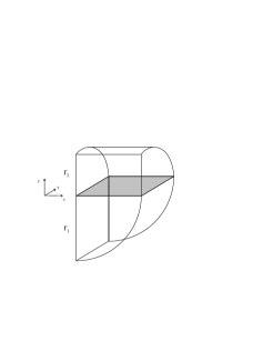
FIG. 1.: Desymmetrized version of the three-dimensional generalized stadium billiard. The plane $z=0$ is shaded.

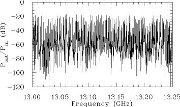
FIG. 2.: Typical transmission spectrum for the frequency range 13-13.25 GHz, where the resonances are still well separated.

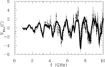
FIG. 3.: Fluctuating part of the experimentally obtained staircase function (dashed line) compared to the fluctuating part of the staircase function for the non-generic modes (full line). We only show that range of the spectrum where both curves are distinguishable.

FIG. 4.: Length spectra from the experimental data (top) compared to (middle) the sum of non-generic modes [from Eq. (1)] plus the unstable periodic orbits [trace formula (3) of Balian and Duplantier], and the unstable periodic orbits (bottom). Diamonds mark those peaks that are assigned to periodic orbits in the plane $z=0$.

FIG. 5.: Left figures: Experimental level-spacing distribution (histogram) and $\Delta_{3}$-statistics (diamonds) for the frequency range 5-10 GHz ($\lambda=0.352$) compared to GOE (full line) and the predictions from the model (see Eq. (2)) (dashed line). Right figures: Same as left figures but for the frequency range 18-18.5 GHz ($\lambda=0.658$).

REFERENCES

- [1] Y. G. Sinai, Russian Math. Surveys (2) 25, 137 (1970); M. V. Berry, Eur. J. Phys. 2, 91 (1981); L. A. Bunimovich, Chaos 1, 187 (1991).
- [2] O. Bohigas, M. J. Gianonni, and C. Schmit, in Quantum Chaos and Statistical Nuclear Physics, edited by T. H. Seligman, H. Nishioka (Springer, Berlin, 1986); E. Heller, in Chaos and Quantum Physics, edited by M.-J. Giannoni, A. Voros, J. Zinn-Justin (Elsevier, Amsterdam, 1991).
- [3] H.-J. Stöckmann, Quantum Chaos: an introduction, (Cambridge University Press, Cambridge, England, 1999).
- [4] H.-D. Gräf et al., Phys. Rev. Lett.69, 1296 (1992).
- [5] M. C. Gutzwiller, J. Math. Phys. 12, 343 (1971).
- [6] D. Ullmo, M. Grinberg, and S. Tomsovic, Phys. Rev E 54, 136 (1996).
- [7] C. Dembowski et al., Phys. Rev. Lett.86, 3284 (2001).
- [8] H. Primack and U. Smilansky, Phys. Rev. Lett.74, 4831 (1995); Phys. Rep. 327, 1 (2000).
- [9] T. Prosen, Phys. Lett. A 233, 323 (1997), ibid. 332.
- [10] O. Frank and B. Eckhardt, Phys. Rev. E53, 4166 (1996).
- [11] R. L. Weaver, J. Acoust. Soc. Am. 85, 1005 (1989); C. Ellegaard et al., Phys. Rev. Lett.75, 1546 (1995); S. Deus, P. M. Koch, and L. Sirko, Phys. Rev. E52, 1146 (1995).
- [12] H. Alt et al., Phys. Rev. E54, 2303 (1996).
- [13] H. Alt et al., Phys. Rev. Lett.79, 1026 (1997).
- [14] R. Balian and B. Duplantier, Ann. Phys. 104, 300 (1977).
- [15] T. Papenbrock, Phys. Rev. E61, 4626 (2000).
- [16] W. Lukosz, Z. Phys. 262, 327 (1973).
- [17] T. Papenbrock and T. Prosen, Phys. Rev. Lett.84, 262 (2000).
- [18] Y. Y. Bai et al., Phys. Rev. A31, 2821 (1985).
- [19] M. L. Mehta Random Matrices, 2nd ed. (Academic Press, San Diego, 1991).
- [20] O. Bohigas, M. J. Giannoni, and C. Schmit, Phys. Rev. Lett. 52, 1 (1984).
- [21] T. Guhr, A. Müller-Groeling, and H. A. Weidenmüller, Phys. Rep. 299, 189 (1998).
- [22] N. Rosenzweig and C. E. Porter, Phys. Rev. 120, 1698 (1960).
- [23] H. Alt et al., Phys. Rev. Lett.81, 4847 (1998).
- [24] H. L. Harney, A. Richter, and H. A. Weidenmüller, Rev. Mod. Phys. 58, 607 (1986).
- [25] M. Sieber et al., J. Phys. A 26, 6217 (1993).
- [26] M. Sieber, Nonlinearity 11, 1607 (1998).