Statistics of Self-Crossings and Avoided Crossings of Periodic Orbits in the Hadamard-Gutzwiller Model

Abstract

Employing symbolic dynamics for geodesic motion on the tesselated pseudosphere, the so-called Hadamard-Gutzwiller model, we construct extremely long periodic orbits without compromising accuracy. We establish criteria for such long orbits to behave ergodically and to yield reliable statistics for self-crossings and avoided crossings. Self-encounters of periodic orbits are reflected in certain patterns within symbol sequences, and these allow for analytic treatment of the crossing statistics. In particular, the distributions of crossing angles and avoided-crossing widths thus come out as related by analytic continuation. Moreover, the action difference for Sieber-Richter pairs of orbits (one orbit has a self-crossing which the other narrowly avoids and otherwise the orbits look very nearly the same) results to all orders in the crossing angle. These findings may be helpful for extending the work of Sieber and Richter towards a fuller understanding of the classical basis of quantum spectral fluctuations.

I Introduction

Billiards on surfaces of negative curvature were first investigated by J. Hadamard [1]. The case of constant negative curvature, known as the pseudosphere, has enjoyed considerable popularity since Gutzwiller’s realization [2] of its potential as a paradigm of quantum chaos. Complete hyperbolicity, the availability of symbolic dynamics, the equality of the Lyapunov exponents of all periodic orbits, and the validity of Selberg’s trace formula are among the attractive features of that system. Useful introductions can be found in Refs. [3, 4, 5, 6]. For a tesselation by maximally desymmetrized octagons (see below) Aurich and Steiner found the spectral fluctuations of the quantum energy spectrum faithful to the Gaussian orthogonal ensemble (GOE) of random-matrix theory [7], as illustrated in Fig. 1 for the so-called form factor, the Fourier transform of the energy dependent two-point correlator of the density of levels.

One of the urgent problems in quantum chaology is to understand the rather universal validity of random-matrix type spectral fluctuations for chaotic dynamical systems, nowadays known as the Bohigas-Giannoni-Schmit conjecture [8]. An important first step was made by Berry [9] on the basis of Gutzwiller’s trace formula [10] which expresses the oscillatory part of the density of energy levels as a sum over periodic orbits, $d_{{\rm osc}}(E)=\mbox{Re}\sum_{\gamma}A_{\gamma}{\rm e}^{{\rm i}S_{\gamma}/\hbar}$, with $S_{\gamma}$ the action and $A_{\gamma}$ a classical stability amplitude of the periodic orbit $\gamma$. Berry realized that the double sum over periodic orbits in the form factor, which involves the building block $A_{\gamma}A_{\gamma^{\prime}}^{*}{\rm e}^{{\rm i}(S_{\gamma}-S_{\gamma^{\prime}})/\hbar}$ in each summand, must draw an important contribution from the diagonal terms $\gamma=\gamma^{\prime}$ since pairs of orbits with action differences larger than Planck’s unit $\hbar$ can be expected to interfere destructively and thus to cancel in the form factor. For time reversal invariant systems each orbit $\gamma$ and its time reverse $\gamma^{\rm TR}$ have equal action such that Berry’s “diagonal approximation” generalizes to include pairs of mutually time reversed orbits and then gives the time dependent form factor as $K(\tau)=2\tau+\ldots$ where $\tau$ is the time in units of the so called Heisenberg time, which is given in terms of the mean level density $\bar{d}(E)$ as $T_{\rm H}(E)=2\pi\hbar\bar{d}(E)$.

Recently, Sieber and Richter [11, 12] employed the pseudosphere in their pioneering move beyond the diagonal approximation; they found a one-parameter family of orbit pairs within which the action difference can be steered to zero. One orbit within each “Sieber-Richter pair” undergoes a small-angle self-crossing which the partner orbit narrowly avoids. The form factor receives the contribution $K_{\rm off}^{1}(\tau)=-2\tau^{2}$ from the family. Together with Berry’s $K_{\rm diag}(\tau)=2\tau$ we thus have a semiclassical understanding of at least the first two terms in the Taylor series of the random-matrix form factor [13] $K_{\rm GOE}(\tau)=2\tau-\tau\ln(1+2\tau)$. The search is now on for further families of orbit pairs which might yield the higher-order terms of the expansion. At the same time, one would like and will eventually have to go beyond the pseudosphere, in order to find the conditions for universal behavior; interesting first steps have been taken for quantum graphs [14] and other billiards [15].

In the present paper we remain with the pseudosphere for a thorough investigation of action correlations which we feel necessary as a basis for further progress towards an understanding of the random-matrix like spectral fluctuations in this prototypical dynamical system (and beyond). We shall make extensive use of symbolic dynamics in (i) establishing a certain local character of the relation between an orbit and its symbol sequence (only a section of the symbol sequence is necessary to determine the associated section of the orbit), (ii) constructing very long periodic orbits (up to hundreds of thousands of symbols) with full control of accuracy, (iii) identifying the ergodic ones among them and establishing a simple and instructive rederivation of Huber’s exponential-proliferation law, (iv) expressing the angle $\epsilon$ of a self-crossing and the closest-approach distance $\delta$ in the partner orbit of a Sieber-Richter pair in terms of the Möbius-transformation matrices associated with the loops joined in a crossing, (v) revealing a useful analytic-continuation kinship of $\epsilon$ and $\delta$, (vi) explicitly relating the joint density $P(\epsilon,l|L)$ for crossing angles and loop lengths $l$ in orbits of total length $L$ to the associated density $P^{a}(\delta,l|L)$ for avoided crossings, and (vii) constructing an expression for the action difference of a Sieber-Richter pair valid to all orders in $\epsilon$.

Some of our findings are based on (overwhelming and exceptionless) numerical evidence based on large numbers of long periodic orbits and thus call for mathematical substantiation.

Even though we strictly confine ourselves to the pseudosphere we expect (and have indeed begun to check) generalizability to other systems for which symbolic dynamics is available.

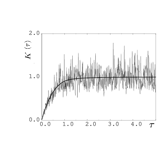
FIG. 1.: Form factor $K(\tau)$ for an asymmetric octagon based on energy levels determined by Aurich and Steiner [7], after averaging over a time window $\Delta\tau=0.01$. Smooth line for GOE.

II The Hadamard-Gutzwiller model

The Hadamard-Gutzwiller model [4, 7] is a two-dimensional billiard on the so called Poincaré disc, i.e. the unit disc $x^{2}+y^{2}=|z|^{2}\leq 1$ endowed with the metric

$$ds^{2}=4\frac{dx^{2}+dy^{2}}{(1-x^{2}-y^{2})^{2}}=4\frac{dzdz^{*}}{(1-|z|^{2})^{2}}\,.$$ (1)

The distance $d(z_{1},z_{2})$ between two points $z_{1},z_{2}$, measured along the unique geodesic connecting them, reads

$$\cosh d(z_{1},z_{2})=1+\frac{2|z_{1}-z_{2}|^{2}}{(1-|z_{1}|^{2})(1-|z_{2}|^{2})}\,.$$ (2)

The geodesics are circles intersecting the boundary at right angles. The total length of the geodesics between its two crossing points with the disc boundary is infinite signaling non-compactness. Free motion on that space is completely hyperbolic. All trajectories (geodesics) have the same Lyapunov exponent, $\lambda=1$, and that fact makes for great simplifications as compared to usual billiards in flat space. The Poincaré disc can be regarded as the stereographic projection of the pseudosphere, the surface of constant negative curvature.

The symmetry of the Poincaré disc is described by the non-compact Lorentz group $SU(1,1)$; we shall only be interested in its hyperbolic elements which are matrices with the structure

$${\cal M}=\left(\begin{array}[]{cc}\alpha&\beta\\ \beta^{*}&\alpha^{*}\end{array}\right)\,,\quad|\alpha|^{2}-|\beta|^{2}=1\,,\quad|{\rm Re}\,\alpha|>1\,.$$ (3)

Their action on points of the complex plane is defined as the Möbius transformation

$$z^{\prime}={\cal M}(z):=\frac{\alpha z+\beta}{\beta^{*}z+\alpha^{*}}\,.$$ (4)

Inner points of the Poincaré disc are transformed to inner points, and boundary points $|z|=1$ to boundary points. Two boundary points $z_{S},z_{U}$ remain invariant, $z_{S}={\cal M}(z_{S})$ and similar for $z_{U}$; the indices signaling “stable” and “unstable”. Using ${\rm det}\ {\cal M}=1$ we find

$$z_{S,U}=\frac{1}{2\beta^{*}}\Big{(}\alpha-\alpha^{*}\pm\sqrt{(\alpha+\alpha^{*})^{2}-4}\Big{)}$$ (5)

where $S$ refers to the $+$ sign, and $U$ to the $-$ sign in the case ${\rm Re}\,\alpha>1$; if ${\rm Re}\,\alpha<-1$ the opposite sign assignment applies. Repeated application of the transformation ${\cal M}$ on any point $z$ leads to the stable fixed point, ${\cal M}^{k}(z)\rightarrow z_{S}$ for $k=1,2,3,\ldots$, while iteration of the inverse map leads to the unstable fixed point, ${\cal M}^{-k}(z)\rightarrow z_{U}$.

The geodesic passing through $z_{S}$ and $z_{U}$ (to be called the “own” geodesic of the matrix ${\cal M}$) is invariant with respect to ${\cal M}$: if $z$ belongs to this geodesic then so does $z^{\prime}={\cal M}(z)$. The distance $d(z,{\cal M}(z))$ is the same for all points of the geodesic and equals

$$L=d(z,z^{\prime})=2\mbox{arccosh}\frac{|\mbox{ Tr }{\cal M}|}{2}\,.$$ (6)

The inverse ${\cal M}^{-1}$ of a matrix ${\cal M}$ is obtained by the replacement $\alpha\to\alpha^{*},\beta\to-\beta$ in (3). These two matrices have their stable and unstable points interchanged. Consequently, a matrix and its inverse shift points along their common “own” geodesic by the same distance but in opposite directions.

To obtain a model with compact configuration space the Poincaré disc is tesselated with tiles of equal area and shape. Each type of tesselation is connected with a particular discrete infinite subgroup $\Gamma$ of $SU(1,1)$ such that by acting on all inner points of a tile by some fixed matrix ${\cal W}\neq{\bf 1}$ we get all inner points of some other tile; the boundaries are mapped to boundaries of the same or other tiles. Using all ${\cal W}\in\Gamma$ we get all tiles and restore the whole disc from a single initial tile. A particular tile is distinguished by containing the origin $z=0$ and is called the fundamental domain. In fact, different tiles are identified by identifying each point $z$ of the Poincaré disc with all its images ${\cal W}(z)$, and so a compact configuration space is indeed arrived at.

In the present paper we exclusively work with octagonal tiles which are all identified with the fundamental domain. The opposite sides of the latter are glued together such that we arrive at a Riemann surface of genus 2, i.e. a two-hole doughnut. Matrices ${\cal W}$ giving rise to octagonal tiles are arbitrary products of four elementary group elements $l_{0},l_{1},l_{2},l_{3}\in SU(1,1)$ and their inverses. For simplicity, we shall mostly consider tesselation with “regular octagons ” (Fig. 2) which have the highest possible symmetry; the pertinent elementary matrices $l_{k},\,k=0,1,2,3,$ are

$$l_{k}=\left(\begin{array}[]{cc}1+\sqrt{2}&\sqrt{2+2\sqrt{2}}\,{\rm e}^{{\rm i}\pi k/4}\\ \sqrt{2+2\sqrt{2}}\,{\rm e}^{-{\rm i}\pi k/4}&1+\sqrt{2}\end{array}\right)\;$$ (7)

and their inverses. The inverse of $l_{k}$ is easily checked to be $l_{k+4}$. Since the index $k$ describes a phase in the off-diagonal matrix elements we conclude

$$l_{k}^{-1}=l_{k+4}=l_{(k+4){\rm\mbox{ }mod\mbox{ }}8}\equiv l_{\bar{k}}\,,$$ (8)

where we have introduced $\bar{k}=(k+4){\rm\mbox{ }mod\mbox{ }}8$. The full set of elementary matrices is thus $l_{k},\,k=0,\ldots,7$.

The sides of the boundary of the fundamental domain can now be labeled $0,1,\ldots,7$ and constructed as follows. Tesselation identifies opposite sides of the regular octagon as 0 $\equiv$ 4, 1 $\equiv$ 5, 2 $\equiv$ 6, and 3 $\equiv$ 7. Points on side $k+4$ are thus images of their mirror symmetric counterparts on side $k$; the group element responsible for such imaging is $l_{k+4}$. In particular, the points on side 0 solve the quadratic equation $l_{4}(z)=-z^{*}$ and form a circle of radius $\left(2^{-1/2}-2^{-1}\right)^{1/2}$, which is in fact a geodesic. Side $k$ is obtained by a rotation of side 0 by $k\pi/8$.

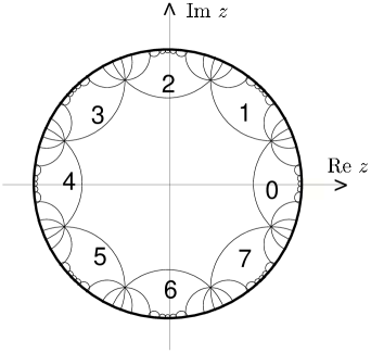
FIG. 2.: Poincaré disc and its tesselation with regular octagons.

Elementary matrices other than $l_{k+4}$ lead from points on side $k$ of the fundamental domain to boundary sides in the next generation of tiles, which may be called ”higher Brillouin zones”, using an analogy with periodic lattices. Obviously, there are eight Brillouin zones neighboring to the fundamental domain. In all other Brillouin zones of all generations, opposite sides are still identified. All Brillouin zones have the same octagonal shape and the same area as the fundamental domain; their visual difference in size and form is caused by the metric (1).

In what follows, we shall often call the elementary matrices $l_{k}$ ”letters”, and their products $l_{j_{1}}l_{j_{2}}l_{j_{3}}\ldots l_{j_{n}}$ ”words”. As a convenient shorthand for a word we shall also employ just the string of indices of the letters, i.e. ${\cal W}=l_{j_{1}}l_{j_{2}}l_{j_{3}}\ldots l_{j_{n}}\equiv(j_{1},j_{2},j_{3},\ldots j_{n})$.

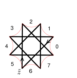
FIG. 3.: Corner points identified by the group identity (9); starting from ${\tilde{z}}$ and following the arrow, the identity can be read off.

As already mentioned, the identification of points $z\equiv{\cal W}(z)$ implies gluing together opposite sides of the octagon; the result is a Riemann surface of genus $2$. On that surface, the eight corner points of the octagon in the unit disc coincide. The identification of the corner points is shown in Fig. 3 . Starting from any corner, (for instance ${\tilde{z}}$ in the figure), taking into account that elementary matrices map opposite points of the boundaries of the fundamental domain onto each other, we go through all corners and come back after eight steps, and read off $l_{5}l_{0}l_{3}l_{6}l_{1}l_{4}l_{7}l_{2}({\tilde{z}})={\tilde{z}}$. Due to the fact that the fixed-point equation ${\cal W}(z)=z$ for ${\cal W}\neq{1\,0\choose 0\,1}$ has unimodular solutions $|z_{S,U}|=1$, we conclude that the matrix product $l_{5}l_{0}l_{3}l_{6}l_{1}l_{4}l_{7}l_{2}$ must be the identity, since the corner point ${\tilde{z}}$ obviously fulfills ${\tilde{z}}\neq 1$ . In fact, using the explicit form (7) of the $l_{k}$, one checks that the foregoing product of eight matrices is the $2\times 2$ unit matrix,

$$l_{5}l_{0}l_{3}l_{6}l_{1}l_{4}l_{7}l_{2}\equiv(5,0,3,6,1,4,7,2)={1\,0\choose 0\,1}=\mathbf{1}\,.$$ (9)

Any geodesic in the tesselated unit disc can be folded into the fundamental domain where it will look like a sequence of disjoint circular segments starting and ending on the boundaries of the octagon. Of course, when the fundamental tile is regarded as a surface of genus 2 the circular sections in question no longer appear as disjoint: A trajectory leaving the fundamental domain through one of the eight sides of the octagon and reentering on the opposite side appears as a smooth curve on the genus 2 surface. It is only after representing the whole unit disc by a single tile with opposite sides glued together (or, equivalently by a surface of genus 2) that a geodesic is capable of self-crossings.

Consider now inertial motion along the “own” geodesic of a matrix ${\cal W}\in\Gamma$. Any point $z$ of the geodesic and its image ${\cal W}(z)$ ( which we know to belong to the same geodesic) are identified by the tesselation. Geodesically moving from $z$ to ${\cal W}(z)$ we are in fact traversing a periodic orbit associated with ${\cal W}$, and the length of that periodic orbit is given by (6); the time reversed orbit is similarly associated with the matrix ${\cal W}^{-1}$. Since each ${\cal W}\in\Gamma$ can be written as a product of elementary matrices ${\cal W}=l_{j_{1}}l_{j_{2}}\ldots l_{j_{n}}$ and encoded by the symbolic word $\{j_{1},l_{2},\ldots l_{n}\}$ we have in fact symbolic dynamics at our disposal as a tool for investigating of periodic orbits.

All matrices from an equivalence class ${\cal Z}{\cal W}{\cal Z}^{-1}$, where ${\cal Z}$ is any matrix from $\Gamma$, have their “own” geodesics identified by tesselation; there is thus one and one only periodic orbit per equivalence class in $\Gamma$. An infinite number of words pertaining to the same equivalence class and thus referring to the same periodic orbit can be obtained from one representative word ${\cal W}=(j_{1},j_{2},j_{3},...j_{r})$; this is done by cyclic permutations of the letters, by similarity transforms (replacing ${\cal W}$ by the longer word ${\cal Z}{\cal W}{\cal Z}^{\rm TR}$ where ${\cal Z}$ is another word, and its associate ${\cal Z}^{\rm TR}={\cal Z}^{-1}$ stands for the matrix inverse to the one represented by ${\cal Z}$; the superscript “TR” is read as “time reversed”), and by using the group identity (9) in all its various forms. A code of the time reversed periodic orbit is produced from the original ${\cal W}$ by writing its symbols $j_{i}$ in the opposite order and replacing each $j_{i}$ by $\bar{j}_{i}=j_{i}+4\mbox{ mod }8$.

Like any geodesic the periodic orbit can be folded into the fundamental domain where it will consist of a finite number $n$ of disjoined circular segments. After that a distinguished $n$-letter word can be introduced for the orbit which is simply the sequence of the “landing” sides of the orbit segments. (The “launching” side is always opposite to the “landing” side of the preceding segment and is not admitted to the symbolic code.) This encoding contains the least possible number of symbols among all members of the equivalence class, and is unique up to cyclic permutations. All $n$ “own” geodesics of a matrix ${\cal W}$ encoded by the distinguished word and its cyclic permutations, cross the fundamental domain.

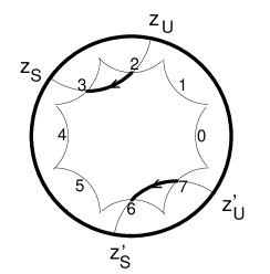
FIG. 4.: Two equivalent geodesics depicting the periodic orbit $(3,6)$; they connect the fixed points $z_{U},z_{S}$ of $l_{3}l_{6}$ and $z_{U}^{\prime},z_{S}^{\prime}$ of $l_{6}l_{3}$. The primitive orbit inside the octagon (bold parts of the geodesics) has two segments.

As an example of how to construct an orbit from its symbol sequence we consider the word ${\cal W}=(3,6)$. Its “own” geodesic can be found calculating the matrix product $l_{3}l_{6}$ and geodesically joining the respective fixed points (Eq.(5)), the curve $z_{S}z_{U}$ in Fig. 4. The full orbit within the fundamental domain could be obtained by folding the geodesic $z_{S}z_{U}$ back into that domain. However, it is easier to find the“own” geodesic of the cyclicly permuted matrix ${\cal W}^{\prime}=l_{6}l_{3}$ and joining its fixed points $z_{S,U}^{\prime}$. The orbit in the fundamental domain is now given by the “inner parts” of the two geodesics (bold intervals of $z_{S}z_{U}$ and $z_{S}^{\prime}z_{U}^{\prime}$ in Fig. 4 ). The “non-primed” segment of the orbit starts on side 2 and ends on side 3, while the “primed” one starts on 7 and ends on 6. The time reversed orbit would have the launching and landing sides interchanged such that its word would be $(2,7)$.

Tesselation with less symmetric octagons, also corresponding to a genus 2 Riemann surface, can be implemented with four elementary matrices $l_{j}\in SU(1,1)$ and their inverses $l_{\bar{j}}$, chosen such that all eight matrices obey the group identity (9). Interestingly, completely desymmetrized genus 2 surfaces do not exist: the inversion symmetry under $z\to-z$ can only be destroyed for $g\geq 3$ [16].

III Construction of long periodic orbits

We here propose a new method for constructing very long periodic orbits. Let us consider a many-letter word ${\cal W}=(j_{1},j_{2},j_{3},...j_{n})$ and its matrix $l_{j_{1}}l_{j_{2}}l_{j_{3}}...l_{j_{n}}$. In order to explicitly construct the associated periodic orbit we can proceed stepwise, so as to determine each of the $n$ circular segments separately. Each step uses only part of the word ${\cal W}$ (the symbol assigned to a segment and its near neighbors); the necessary length of that part is determined by the required accuracy and not at all by the length of ${\cal W}$.

In the preceding section, we discussed the connection between the fixed points $z_{S},z_{U}$ of the Möbius transformation associated with ${\cal W}=l_{j_{1}}l_{j_{2}}l_{j_{3}}...l_{j_{n}}$ and the periodic orbit. We would also like to recall that the two fixed points determine the circular segment associated with the first letter $l_{j_{1}}$ of the word; to find the next circular segment one has to determine the two fixed points for the equivalent word obtained by cyclically permuting $l_{j_{1}}$ to the right end. This is how all $n$ circular segments of the orbit in question can be found, one after the other.

It is convenient to first determine the stable fixed point for the first circular segment. To that end, we consider the sequence of matrices $\{{\cal W}_{1}=l_{j_{1}},{\cal W}_{2}=l_{j_{1}}l_{j_{2}},{\cal W}_{3}=l_{j_{1}}l_{j_{2}}l_{j_{3}},\ldots\}$ which are obtained by truncating ${\cal W}$. For each matrix in the sequence we solve the quadratic fixed-point equation. The sequence of unstable fixed points thus obtained behaves erratically. The sequence of stable fixed points, however, converges rapidly, in fact with exponentially growing accuracy. The limiting point itself is none other than the stable fixed point $z_{S}$ of the whole word beginning with $l_{j_{1}}$.

The convergence of the series of stable fixed points of ${\cal W}_{k}$ can be ascertained analytically. To that end we first observe that the matrix ${\cal W}_{k}$ has its elements grow exponentially with the length $L$ of its corresponding periodic orbit. This is obvious from the relation (6) of the length of an orbit to the trace of its matrix, $|{\rm Tr}\ {\cal W}_{k}|=2\cosh(L_{k}/2)\approx{\rm e}^{L_{k}/2}$, and from the unimodularity of the determinant, ${\rm det}\ {\cal W}_{k}=\alpha\alpha^{*}-\beta\beta^{*}=1$. While under other circumstances such exponential growth gives rise to inaccuracy growing out of control, we can now rejoice in the growth working in our favor when determining the stable fixed point of ${\cal W}$: For large matrix elements, Eq. (5) simplifies to

$$z_{S}\approx\frac{\alpha}{\beta^{*}}\ \ \ \ \ \ \ \ z_{U}\approx-\frac{\alpha^{*}}{\beta^{*}}\,.$$ (10)

When proceeding to ${\cal W}_{k+1}$ by including the letter $l_{j_{k+1}}=\left({l_{11}\atop l_{12}^{*}}{l_{12}\atop l_{11}^{*}}\right)$ and comparing the stable fixed points $z_{S}^{k},\,z_{S}^{k+1}$ of ${\cal W}_{k}=\left({\alpha\atop\beta^{*}}{\beta\atop\alpha^{*}}\right),\,{\cal W}_{k+1}={\cal W}_{k}l_{j_{k+1}}$, we find for their difference, using the approximation (10) and the unimodularity of $\det{\cal W}_{k}$,

$$z_{S}^{k}-z_{S}^{k+1}=\frac{l_{12}^{*}}{\beta^{*}(\beta^{*}l_{11}+\alpha^{*}l_{12}^{*})}\,.$$ (11)

Since the elements $l_{ij}$ are of order unity, the difference $z_{S}^{k}-z_{S}^{k+1}$ is of order ${\rm e}^{-L_{k}}$, i.e. small once the word ${\cal W}_{k}$ is long. Exponentially fast convergence of the sequence $z_{S}^{k}$ is thus obvious.

We can now turn to the task of determining the unstable fixed point of $\cal W$. As explained in the last section, the time reversed orbit is obtained using the reversed Möbius transformation matrix ${\cal W^{\rm TR}}={\cal W}^{-1}$, which has stable and unstable fixed points interchanged relative to ${\cal W}$. Consequently, we get the unstable fixed point of the circular segment of ${\cal W}$ associated with the letter $l_{j_{1}}$ as the limit of the sequence of stable fixed points of the matrices $\{l_{j_{n}}^{-1},l_{j_{n}}^{-1}l_{j_{n-1}}^{-1},l_{j_{n}}^{-1}l_{j_{n-1}}^{-1}l_{j_{n-2}}^{-1},\ldots\}$; these matrices are truncations of ${\cal W}^{\rm TR}$. The sequence of stable fixed points of these truncations converges as rapidly as the one considered before and yields the unstable fixed point $z_{U}$ for the first circular segment of ${\cal W}$.

With both $z_{U}$ and $z_{S}$ determined to the desired accuracy for the segment of the orbit corresponding to $l_{j_{1}}$, one repeats the procedure for the subsequent circular segment, i.e. the one corresponding to $l_{j_{2}}$.

As an obvious property of our method, we find that the computational effort needed to construct a periodic orbit with $n\gg 1$ symbols grows only linearly with $n$. More importantly, we only have to do local work for local properties: Each of the $n$ circular segments of the orbit inside the fundamental domain is found with a number of operations independent of $n$; for each segment one has to calculate a product of a moderate number of elementary matrices (about 18 for a 15-digit accuracy). As we proceed segmentwise, no inaccuracy can accumulate. There is thus practically no limit on the length of the accessible orbits. For example, we had no difficulty in calculating a periodic orbit corresponding to a sequence of $10^{5}$ randomly selected symbols.

It may be useful to again comment on the fact that any periodic orbit is, in principle, determined by any one of its circular segments within the fundamental domain. One just has to take the full geodesic running between the fixed points $z_{U},z_{S}$, to which the segment belongs, and fold that geodesi c into the fundamental domain. However, such folding is numerically unstable and cannot be implemented with finite precision for very long orbits.

Inasmuch as we work with fixed points of Möbius transformations, our method seems to be restricted to the Hadamard-Gutzwiller model. However, underlying all technicalities is a locality in the relationship between orbits and symbolic words, and that locality does in fact make our method generalizable, as will be explained in a separate publication.

IV Pruning

The locality of the word-orbit relationship makes our method a promising pruning tool. Pruning generally means recognizing and deleting symbolic words not corresponding to physically realizable orbits [17]. In the Hadamard-Gutzwiller model every word ${\cal W}$ does correspond to an allowed orbit. On the other hand, there are infinitely many equivalent words which must be counted only once whenever sums over orbits are to be taken, as for instance in Selberg’s trace formula. The particular word we are interested in is simply the ordered list of “landing sides” of the regular octagon for the succession of circular segments of the orbit (Section II). The task of selecting this distinguished word can be regarded as a variant of pruning.

A first step is to discard words which can be shortened, considering that the distinguished representation contains the least possible number of symbols; in particular, the word must not contain pairs of symbols $k{\bar{k}}$ with ${\bar{k}}=(k+4){\rm\mbox{ }mod\mbox{ }}8$. The group identity (9) is yet another source of “badness”: Whenever it allows to replace a word by an equivalent shorter one, only the latter needs to be further scrutinized.

Real problems are due to the fact that the group identity (9) allows to write some four-letter parts of words in reversed order, e.g. $(0,5,2,7)=(7,2,5,0)$. The average number of such reversible 4-sequences in a word with $n$ random symbols is estimated in Appendix A as $0.0043n$. Each of the 4-sequences must have a uniquely defined direction in the distinguished word; it is not known a priori, however, which direction is the “correct” one. The suitable word has thus to be selected among $2^{0.0043n}$ candidates. For, say, $n\sim 10^{5}$ no hope can be set on any trial-and-error procedure like building the orbits corresponding to the equivalent words one by one and discarding those not lying inside the fundamental domain.

With our algorithm we had no problem finding the correct direction of the $4$-letter sequences just mentioned. Whenever at some stage our method produced an arc which did not cross the fundamental domain, the letter for that arc turned up within a reversible $4$-sequence. Upon reversing that particular $4$-sequence (out of the thousands present in the code!) the arc always returned to the fundamental domain, and construction of the periodic orbit could be continued. Pruning thus becomes a local problem, which can be attacked efficiently.

V Ergodic periodic orbits

It is well known that the geodesic flow in the Hadamard-Gutzwiller model is ergodic [4] such that almost all trajectories cover the phase space homogeneously. Introducing limited phase-space resolution we can extend the notion of ergodicity to periodic orbits: Almost all sufficiently long periodic orbits cover the coarse-grained phase space uniformly.

The overwhelming prevalence of ergodic periodic orbits does not imply that a random sequence of uncorrelated symbols must yield an ergodic orbit. In fact, practically every periodic orbit so constructed is extremely non-ergodic, as illustrated in Fig. 5(a) by the configuration-space density for 100000 randomly chosen symbols; the grossly non-uniform density thus incurred is anything but ergodic.

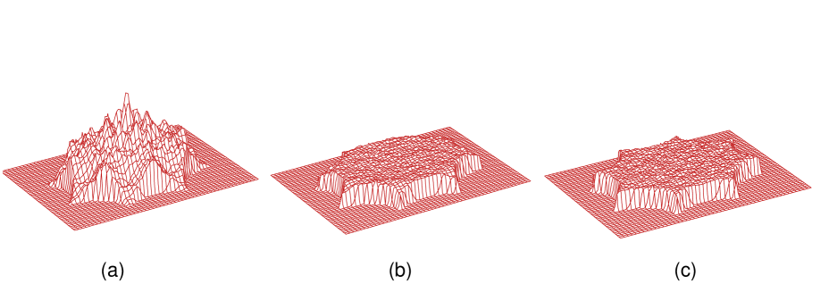
FIG. 5.: Coverage of fundamental domain by three periodic 100000-symbol orbits: (a) Random symbol sequence yields extremely inhomogeneous distribution. (b) Account of two-step correlations gives almost ergodic distribution, with small deviations only near octagon corners. (c) Symbol sequence imported from non-periodic trajectory gives uniform density.

In configuration space, a long periodic orbit intersects itself many times, and the distribution of self-crossing angles $\epsilon$ provides another sensitive test for ergodicity. We shall consider it in some detail because of its role in the Sieber-Richter theory. The angle $\epsilon$, defined to lie in the interval $0\leq\epsilon<\pi$, is complementary to the angle between the velocities at the crossing; see Fig. 6. The number of self-crossings with crossing angles in the interval $(\epsilon,\epsilon+d\epsilon)$ in periodic orbits of length $L$ yields a density $P(\epsilon|L)$. Since no direction is distinguished the probability that an element $d{\vec{l}}_{1}$ of the orbit intersects with the element $d{\vec{l}}_{2}$ is given by the geometric projection $P(\epsilon|L)\propto|d{\vec{l}}_{1}\times d{\vec{l}}_{2}|\propto\sin\epsilon$. Comparing that prediction with the plot of $P(\epsilon|L)$, numerically obtained for our periodic orbit with 100000 randomly chosen symbols, we encounter blatant disagreement, despite the enormous length of the orbit. In particular, for small $\epsilon$, the number $P(\epsilon|L)$ of self-crossings decreases like $\propto\epsilon^{2/3}$ rather than $\propto\epsilon$.

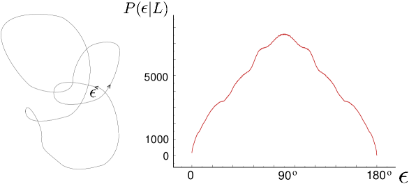
FIG. 6.: Definition of crossing angle $\epsilon$; strongly non-ergodic density $P(\epsilon|L)$ for orbit with $10^{5}$ random symbols.

It is important to stress that the non-ergodic patterns in Figs. 5(a) and 6 are not due to an unlucky choice of the periodic orbit by the random-number generator employed to pick symbols. As we shall see presently, two precautions must be taken for our way towards ergodic periodic orbits. First, we should fix the geometric length $L$ rather than the number $n$ of symbols and, second, wave good-bye to the assumption of uncorrelated symbols.

A Number of symbols vs. orbit length

Within an ensemble of orbits of fixed number of symbols $n$ the orbit length $L$ will fluctuate. Ascribing equal probability to all allowed symbol sequences and invoking, for large $n$, the central limit theorem we have the distribution of $L$ as a Gaussian, with mean and variance both proportional to $n$,

$$g(L|n)=\frac{1}{\sqrt{2\pi n\Delta}}\,{\rm e}^{\frac{(L-nd_{n})^{2}}{2n\Delta}},\ \ \ \ \ \ \ \ \int g(L|n)dL=1\,;$$ (12)

$d_{n}$ and $\Delta$ are the mean length and variance per symbol. The values of these quantities are system specific; using an ensemble of 100000 periodic orbits with $n=100000$ randomly selected symbols each for the regular octagon we numerically find

$$d_{n}\approx 2.2568,\quad\Delta\approx 0.6283\,.$$ (13)

The concentration of $g(L|n)$ in the vicinity of its maximum becomes ever more pronounced as $n$ grows. The mean length per symbol for a long periodic orbit obtained by throwing honest dice for its symbols will therefore almost certainly be very close to $d_{n}$.

Of greater interest is a different ensemble of periodic orbits, which has the length interval $(L)$ fixed rather than the number of symbols $n$. In particular, it is the fixed-length ensemble that one has in mind when speaking about the overwhelming prevalence of ergodic orbits. To find the number of orbits $N(L)dL$ in the length interval $(L,L+dL)$ we need the number of different periodic orbits with $n$ symbols,

$$\nu(n)=\frac{1}{n}p_{\rm eff}^{n}\,,$$ (14)

where the effective number of symbols $p_{\rm eff}=6.98$ deviates only slightly from the naive estimate $8-1=7$ obtained by excluding $k{\bar{k}}$ patterns; the slight deviation is due to the group identity (9); the factor $1/n$ reflects the equivalence of cyclically permuted symbol sequences; a detailed discussion of $p_{\rm eff}$ will be presented in Appendix B. We proceed to $N(L)$ by summing over all possibilities for the length to lie in the interval $(L,L+dL)$ as $N(L)=\sum_{n}g(L|n)\nu(n)$ or, approximating the sum by an integral,

$$N(L)=\int dn\ g(L|n)\nu(n)=\int dn\frac{1}{\sqrt{2\pi n^{3}\Delta}}\,{\rm e}^{n\ln p_{\rm eff}-\frac{(L-nd_{n})^{2}}{2n\Delta}}\,.$$ (15)

In the interesting case of large $L$ the integral can be evaluated using the saddle-point approximation. The saddle of the integrand lies at

$$n_{\rm max}=\frac{L}{\sqrt{d_{n}^{2}-2\Delta\ln p_{\rm eff}}}\,.$$ (16)

FIG. 7.: For fixed number $n$ of symbols, the distribution of orbit lengths is Gaussian (12) with maximum at $<L>=nd_{n}$. However, ergodic orbits are those at $L_{\rm erg}=nd_{L}$, in ultra-left wing of Gaussian.

The orbit density is thus found to obey the familiar exponential proliferation law

$$N(L)=\frac{1}{L}{\rm e}^{\eta L}\,,$$ (17)

with the growth rate

$$\eta=\frac{d_{n}-\sqrt{d_{n}^{2}-2\Delta\ln p_{\rm eff}}}{\Delta}\,.$$ (18)

The latter rate must coincide with the topological entropy. For billiards on surfaces of constant negative curvature that entropy equals unity and (17) becomes Huber’s law [5]. With our approximate numerical values (13) inserted, our expression (18) yields $\eta\approx 1.00026$, in nice agreement with the value $\eta=1$ required by Huber’s law.

The orbits described by the proliferation law (17) are known to be ergodic in their overwhelming majority. Since we have just seen this law to arise mostly from contributions of orbits with the number of symbols close to $n_{\rm max}$, it is clear that the ergodic orbits must have the mean length per symbol given by

$$d_{L}=\frac{L}{n_{\rm max}}=\sqrt{d_{n}^{2}-2\Delta\ln p_{\rm eff}}\,.$$ (19)

For the regular octagon, with its values for $d_{n},\Delta$ given in (13) we have $d_{L}=1.6283$. Note that this latter value strongly deviates from the mean length per symbol $d_{n}=2.2568$ obtained from randomly chosen sequences of $n$ symbols. Therefore, orbits generated using random sequences of $n$ symbols have an exceedingly small probability to be ergodic. To see this we must realize that the orbits constituting the maximum of the integrand in the distribution at fixed length (15) (known to be ergodic) are not those forming the maximum of the Gaussian distribution (12) at fixed number of symbols, but rather belong to its ultra-left wing; the difference of the locations of the maxima of the two distributions in question is of order $L$, while the widths are only of order $\sqrt{L}$.

The enormous difference between the two ensembles is due to the exponential growth of the total number of orbits with $n$ symbols, $\nu(n)$. The orbits with the length per symbol close to $d_{L}$ are in extremely small proportion to all orbits with the same number of symbols. However, they are dominant among the orbits with a given length since they have many more symbols.

The fact that the maximum of the integrand in (15) is formed by ergodic orbits can be regarded as due to a theorem of Bowen’s [18]. The number of orbits within the ergodic subset (characterized by $d_{L}$) grows in the limit $L\to\infty$ as fast as the total number of orbits.

B Symbol correlations in ergodic orbits

Correlations must be accounted for in the symbol sequence if ergodic orbits are to be constructed. We propose to establish such correlations with the help of geometric considerations. The number $dN_{\rm\phi}$ of times an ergodic orbit intersects a line element of infinitesimal length $dl$, with the crossing angle in the interval $(\phi,\phi+d\phi)$, obeys

$$dN_{\phi}\propto\sin\phi\ dld\phi\,.$$ (20)

Indeed, $dN_{\phi}$ and the distribution of self-crossing angles $P(\epsilon|L)$ must have the same sinusoidal angle dependence; for self-crossings the line element $dl$ is a stretch of the periodic orbit itself rather than an element of some fixed line in the billiard. The behavior in question is also similar to the ”cosine law” of optics for the angular distribution of the intensity of light emitted diffusely by some surface element.

We now apply the rule (20) to an element of one side of the regular octagon, say number $0$. The segment of an ergodic orbit launched from that element succeeds the orbit segment with the symbol $4$. In search is now the probability for the orbit segment launched from side 0 to land on side $k$, i.e. the probability $P_{4\to k}$ that a certain symbol $k\neq 0$ follows the symbol $4$ in the symbolic code. An orbit segment is uniquely determined by the position of its initial point on, and the crossing angle with, the “launching side” $0$. We thus find the transition probability by first integrating (20) over the angle range spanned by side $k$ with respect to the launching element, and subsequently integrating along side $0$. Fig. 8 explains the pertinent geometry.

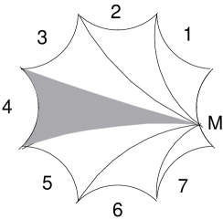
FIG. 8.: Geodesics connecting point $M$ at side $0$ with corners divide octagon into seven sectors. Orbit starting from $M$ with momentum direction within $k$-th sector will arrive at side $k$. Integrating over all such directions and all starting points $M$ on side $0$ gives transition probability $P_{4\to k}$.

For an irregular octagon the procedure just explained must be applied to all launching sides $k_{\mbox{in}}$ to get the probabilities for the symbol $k_{\mbox{in}}$ to be followed by $k_{\mbox{fin}}$. In the regular octagon the transition probabilities depend only on the absolute value of $k_{\mbox{in}}-k_{\mbox{fin}}$ which can be 1,2 or 3; they are to be compared with the value $1/7=0.143\ldots$ which would correspond to the random symbol sequence without correlation.

Alternatively, symbol correlations can be read off non-periodic trajectories with random initial conditions. Both approaches lead to good agreement for the single-step transition probabilities $P_{i\to j}$, as documented in the following table,

theory0.62010.20890.12000.0510nonper. traj.0.61930.20910.12050.0512.fragments theory0.62010.20890.12000.0510nonper. traj.0.61930.20910.12050.0512\displaystyle\begin{tabular}[]{l ||c |c | c | c |}&$P_{4\rightarrow 1}$&$P_{4\rightarrow 2}$&$P_{4\rightarrow 3}$&$P_{4\rightarrow 4}$\\ \hline\cr theory&$0.6201$&$0.2089$&$0.1200$&$0.0510$\\ nonper. traj.&$0.6193$&$0.2091$&$0.1205$&$0.0512$\end{tabular}\,.

P→41P→42P→43P→44P→41P→42P→43P→44 (24)

Symbol sequences respecting the single-step correlations just explained yield periodic orbits exhibiting ergodicity to an impressive degree of approximation. In particular, the average length per symbol of periodic orbits in the regular octagon decreases from 2.257 to 1.694, i.e. a value rather close to the ergodic limit $d_{L}=1.628$.

To further faithfulness to ergodicity we must account for higher correlations in the symbol sequence. The next step involves two-step transition probabilities $P_{i\to j\to k}$, i.e. the conditional probabilities for a certain symbol to follow any given two-symbol sequence. For the regular octagon two-step correlations are embodied in a set of 16 numbers which can be calculated upon suitably refining the geometric reasoning applied above to find the four transition probabilities comprising the single-step correlations. By imposing two-step correlations on the symbol sequence we brought the average length per symbol for periodic orbits down to 1.643; the coverage of configuration space thus obtained is almost uniform, as required by ergodicity; see Fig. 5(b). It is worth noting that $P_{i\to j\to k}$ differ from the product of the single-step transition probabilities $P_{i\to j}P_{j\to k}$ by up to 30%.

An interesting alternative way to account for all correlations of importance is to read off symbol sequences of the desired length from a non-periodic trajectory. The symbolic word thus obtained can be used for generating an almost perfectly ergodic periodic orbit which will almost everywhere coincide, to a high precision, with the corresponding section of the non-periodic trajectory. Only a dozen or so segments of the periodic orbit, namely those corresponding to the beginning and the end of the word, will deviate from the non-periodic progenitor. The ergodicity of the orbit thus produced will be close to perfection, as witnessed by the density distribution in Fig. (5)(c). Moreover, the two trajectories under discussion will have very nearly the same length per symbol; in fact, considering $10^{5}$ orbits with $10^{5}$ symbols each, generated from non-periodic trajectories, we got the average length per symbol as 1.614. The latter value differs slightly from the prediction $d_{L}=1.628$ based on (19) and the numerical data (13) on the ensemble of the orbits with random symbol sequences; we have not bothered to look for an explanation of that (minute) discrepancy.

To finally illustrate the suitability of the mean length per symbol as an indicator of the fidelity of periodic orbits to ergodicity, Fig. 9 depicts the distribution $dN_{\phi}/d\phi$ of the angle $\phi$ between landing side and arriving periodic orbit, for groups of orbits of different mean lengths $d$ per symbol. Such groups were constructed from an ensemble of periodic orbits pertaining to a large fixed number of random uncorrelated symbols. The distribution of lengths $L$ within such an ensemble is the Gaussian depicted in Fig. 7. The approach to ergodicity with $d\to d_{L}$ is clearly visible in Fig. 9

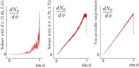
FIG. 9.: Number $dN_{\rm\phi}/d\phi$ of segments landing near some point of side $0$ with angle $\phi$ vs $\phi$, for two different values of mean length $d$ per symbol and for non-periodic trajectories. Fidelity to ergodic sine law (20) increases as $d$ approaches $d_{L}$ of (19).

VI Crossing angles, avoided-crossing widths, and loop lengths

We can now turn to the statistics of self-crossings and associated avoided crossings which is believed to be an important classical ingredient in the explanation of universality of fluctuations in quantum energy spectra of chaotic dynamics [11, 12, 14, 19].

A Crossings

Each crossing divides a periodic orbit of length $L$ into two loops whose lengths $l_{1},l_{2}$ add up to $L$. In what follows, we shall focus on the shorter one and its length $l={\rm min}(l_{1},l_{2})$. For the statistical considerations to follow we employ the number of loops $p(\epsilon,l|L)d\epsilon\ dl$ with lengths in the interval $(l,l+dl)$ and crossing angles in the interval $(\epsilon,\epsilon+d\epsilon)$ in ergodic orbits of length $L$. The density of loop lengths and crossing angles, $p(\epsilon,l|L)$, be calculated analytically for the Hadamard-Gutzwiller model due to the fact that each loop can be continuously deformed to a loop with crossing angle $\pi$, that is, to a periodic orbit $\gamma$, as indicated in Fig. 10. Due to the equality of the Lyapunov exponents for all trajectories in the Hadamard-Gutzwiller model the loop length $l_{\gamma}$ is uniquely determined by the crossing angle $\epsilon$ and the length $L_{\gamma}$ of the periodic orbit $\gamma$ as [11]

$$\cosh\frac{l(\pi)}{2}\equiv\cosh\frac{L_{\gamma}}{2}=\cosh\frac{l(\epsilon)}{2}\sin\frac{\epsilon}{2}\,;$$ (25)

for $L_{\gamma}$ large that relation simplifies to

$$l_{\gamma}(\epsilon)-L_{\gamma}\approx 2\ln\frac{1}{\sin\frac{\epsilon}{2}}\,.$$ (26)

We immediately infer that a loop is longer than its periodic-orbit deformation $\gamma$ by an amount independent of $\gamma$ and the longer the smaller the crossing angle; even for the shortest orbits with the length $L_{0}=3.06$ (the value refers to the regular octagon) the error of the simplified relation (26) relative to (25) is less than 2%.

FIG. 10.: Deformation of loop to periodic orbit.

Using the basic relation (25), Sieber expresses $p(\epsilon,l|L)$ as a sum over periodic orbits [11],

$$p(\epsilon,l|L)=\frac{L}{2\pi A}\sum_{\gamma}\frac{\ L_{\gamma}\ \delta(l-l_{\gamma}(\epsilon))\sin\epsilon}{r_{\gamma}\sqrt{(-1+\cosh L_{\gamma})(-1+\cosh L_{\gamma}+2\cos^{2}\frac{\epsilon}{2})}}\;;$$ (27)

here $r_{\gamma}$ is a repetition number equaling 1 if $\gamma$ is a primitive periodic orbit, and $A=4\pi$ is the area of the octagon. Due to $l_{\gamma}(\epsilon)>L_{\gamma}$ only orbits with $L_{\gamma}<l<L/2$ contribute to the sum.

As $l$ grows, more and more periodic orbits contribute and the sum will eventually be dominated by long orbits for which $2\cosh L_{\gamma}\approx\exp L_{\gamma}\gg 1$ so that the denominator may be replaced by $\exp L_{\gamma}$. Taking into account (26) and applying the sum rule of Hannay and Ozorio de Almeida [20] we obtain the ergodic result,

$$p(\epsilon,l|L)\approx\frac{L}{\pi A}\sin\epsilon,\quad l\gg l_{0}(\epsilon)\;,$$ (28)

where $\cosh(l_{0}(\epsilon/2))=\cosh(L_{0}/2)/\sin(\epsilon/2)$ gives the length of the shortest possible loop created by deformation of the shortest periodic orbit of the system with length $L_{0}$, again according to the basic relation (25).

Two reduced distributions can be obtained from the general expression (27). Integrating over the angle from zero to some $\epsilon_{\rm max}$, we obtain the length distribution $p(l|\epsilon_{\rm max},L)$ for loops with crossing angles smaller than $\epsilon_{\rm max}$ in the periodic orbit of length $L$. The resulting expression is astonishing simple,

$$p(l|\epsilon_{\rm max},L)=\int_{0}^{\epsilon_{\rm max}}p(\epsilon,l|L)d\epsilon=\frac{L}{2\pi A\cosh^{2}\frac{l}{2}}\ \sum_{l_{\gamma}(\epsilon_{\rm max})\leq l}\ \frac{L_{\gamma}}{r_{\gamma}}{\rm coth}\frac{L_{\gamma}}{2}\,.$$ (29)

The only $\epsilon_{\rm max}$-dependence lies in the summation condition $l_{\gamma}(\epsilon_{\rm max})\leq l$ and indicates that only those periodic orbits $\gamma$ contribute to the sum which can be deformed to a loop of length $l_{\gamma}(\epsilon_{\rm max})$ smaller than the given length $l$. Therefore, we obtain a staircase function for the quantity $p(l|\epsilon_{\rm max},L){\cosh^{2}l/2}$. In Fig 11 (a), (c), we display $p(l|\epsilon_{\rm max},L)$ for $\epsilon_{\rm max}=\pi$ and $\epsilon_{\rm max}=\pi/36$, whereas (b) displays the staircase obtained from (a) after multiplication with $\cosh^{2}l/2$; these plots reveal perfect agreement between the numerical results obtained from all loops in an ensemble of $10^{6}$ ergodic periodic orbits with the prediction of the periodic-orbit sum (29).

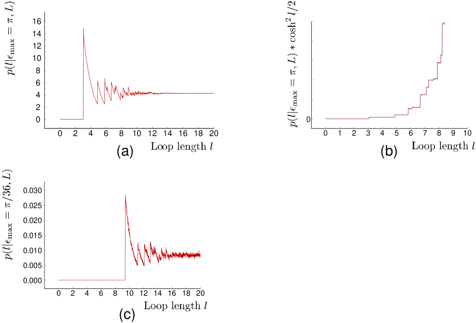
FIG. 11.: Joint density of loop lengths and crossing angles; analytic result (29) for $\epsilon_{\rm max}=\pi$ and $\epsilon_{\rm max}=\pi/36$ indistinguishable from numerical finding. Angle-dependent gap visible in (a) and (c) is origin of logarithmic correction to ergodic behavior of self-crossing distribution.

Note that a gap arises in the length distribution $p(l|\epsilon_{\rm max},L)$ due to the existence of a shortest periodic orbit and the related shortest possible loop of angle $\epsilon$ and length $l_{0}(\epsilon)$. The gap is given by $0\leq l\leq l_{0}(\epsilon_{\rm max})$. In particular, in Fig. 11(a), $l_{0}(\epsilon_{\rm max}=\pi)=L_{0}=3.06$ is just the length of the smallest periodic orbit of the system, whereas in Fig. 11 (c), $l_{0}(\epsilon_{\rm max}=\frac{\pi}{36})=9.41$ is the length of the shortest possible loop with angle $\epsilon_{\rm max}=\pi/36$. Generally, in accord with the relation (26) between the lengths $l_{\gamma}(\epsilon)$ and $L_{\gamma}$, the peaks related to all periodic orbits experience practically the same shift to the right, $\sim 2\ln(2/\epsilon)$; therefore, when $\epsilon_{\rm max}$ is decreased the length distribution appears to shift to the right rather rigidly.

When (27) is integrated over all loop lengths $l$, we obtain the density of crossing angles $P(\epsilon|L)$ in ergodic periodic orbits of length $L$ as

$$P(\epsilon|L)=\int_{0}^{L/2}p(\epsilon,l|L)dl=\frac{L\sin\epsilon}{\pi A}\left(\frac{L}{2}-l_{\rm eff}(\epsilon)\right)\,.$$ (30)

The term in the right hand side proportional to $L^{2}$ could be obtained immediately using the ergodic approximation (28). The actual number of crossings is smaller due to the already mentioned gap in the loop length distribution, such that the effective integration interval in (30) is shorter than $L/2$. This is taken into account by the introduction of the effective minimal loop length $l_{\rm eff}(\epsilon)$; that latter quantity is close to, but somewhat smaller than, the gap visible in Fig 11(a), (c), i.e. the length $l_{0}(\epsilon)$ of the loops related to the shortest periodic orbit. The discrepancy arises from the shortest periodic orbits whose contribution is greatly in excess of the ergodic prediction.

A periodic-orbit sum for $l_{\rm eff}(\epsilon)$ is obtained by substituting the loop length density (27) for the integrand in (30) and comparing the left and right hand sides. Recalling that all loop lengths exceed the lengths of their associated periodic orbits by the same quantity (see (26)) and employing the sum rule, we can make the summation interval independent of $\epsilon$,

$$l_{\rm eff}(\epsilon) = 2\ln\frac{1}{\sin\frac{\epsilon}{2}}+\phi(\epsilon);$$ (31)

$$\phi(\epsilon) \equiv \frac{L}{2}-\sum_{L_{\gamma}<\frac{L}{2}}\frac{L_{\gamma}}{r_{\gamma}\sqrt{(-2+2\cosh L_{\gamma})(-2+2\cosh L_{\gamma}+4\cos^{2}\epsilon/2)}}\;.$$ (32)

For long orbits (large $L$) the last expression is $L$-independent. Indeed, the increment of $\phi(\epsilon)$, when $L$ is replaced by $L+\Delta L$, is given by

$$\Delta\phi\approx\frac{\Delta L}{2}-\sum_{\frac{L}{2}<L_{\gamma}<\frac{L+\Delta L}{2}}L_{\gamma}{\rm e}^{-L_{\gamma}}=0,$$ (33)

which follows from the proliferation law for periodic orbits.

The $\epsilon$ dependence of $\phi(\epsilon)$ comes from the shortest and thus non-generic orbits; it is so weak that for most purposes we can set $\phi(\epsilon)\approx\phi(0)$ and work with

$$l_{\rm eff}(\epsilon)\approx 2\ln\frac{c}{2\sin\frac{\epsilon}{2}},\quad c=2\mbox{e}^{\frac{\phi(0)}{2}}\approx 3.16\,;$$ (34)

the constant $c$ was obtained by choosing $L/2=12$ and correspondingly allowing for periodic orbits with lengths $L_{\gamma}\leq 12$ in $\phi(0)$.

B Avoided Crossings

Inasmuch as every periodic orbit with a small-angle self-intersections has a partner orbit which is almost identical save for avoiding the said crossing, one would expect the statistics of crossings and avoided crossings to be the same, at least in the limit of small angles. In the present subsection we shall confirm that expectation, mainly by showing that there is a formal analytic-continuation relationship between crossings and avoided crossings. However, it is important to notice that two different types of avoided crossings arise which have different properties.

We generalize the considerations of the preceding subsection by imagining the division of a periodic orbit into two “loops” by an avoided crossing. As shown in Fig. 12, two geodesics, the intra-octagon segments of which belong to a periodic orbit, may either cross inside the unit disc once or not at all. As before, we let $\epsilon$ be the angle complementary to the angle between the velocity vectors of the two geodesics at an intersection as defined in Fig. 12 (a). When the direction of velocity in one of the two geodesics is reversed, the role of the angles $(\epsilon,\pi-\epsilon)$ is interchanged. Elementary Euclidian geometry provides the relation between the radii $r_{1},r_{2}$ of the two geodesic circles, the distance $l$ between its midpoints and the angle $\epsilon$ as

$$\sin^{2}\frac{\epsilon}{2}=\frac{1}{2}\pm\frac{r_{1}^{2}+r_{2}^{2}-l^{2}}{4r_{1}r_{2}}\,,$$ (35)

where all quantities are measured in Euclidian units. The two solutions with $\pm$ correspond to the two complementary angles $(\epsilon,\pi-\epsilon)$.

In case the two segments do not cross there exists a minimal distance $\delta$ between them. That distance is measured using the metric (1), along the geodesic orthogonal to the said segments. The two intersection points of this geodesic with the segments of the orbit divide the orbit into two loops, much the same as in the case of a crossing.

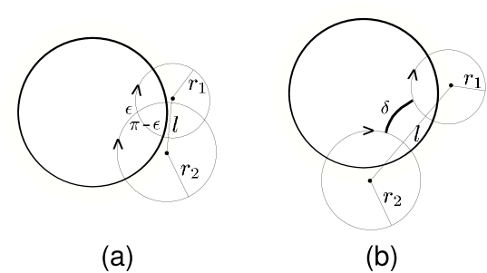
FIG. 12.: Geodesics in unit disc may cross once (a), or form avoided crossing. Part (b) depicts antiparallel avoided crossing; reversion of motion in one geodesic would interchange angles as $\epsilon\leftrightarrow\pi-\epsilon$ in (a) and form parallel avoided crossing in (b).

Surprisingly, the distance $\delta$ is given by analytic continuation ($\epsilon\to{\rm i}\delta$) of equation (35),

$$\sinh^{2}\frac{\delta}{2}=-\frac{1}{2}+\Big{|}\frac{r_{1}^{2}+r_{2}^{2}-l^{2}}{4r_{1}r_{2}}\Big{|}\,,$$ (36)

where, in contrast to $\delta$, the radii $r_{1},r_{2}$ and the distance $l$ are still meant in the Euclidian sense, as in (35). We do not want to pause and give the straightforward but dull proof of (36) here but shall actually recover both (35) and its analytic continuation (36) through symbolic dynamics in Sect. VII.

The geodesic along which the width of an avoided crossing is measured may consist of several disjoint arcs within the fundamental domain; we shall come back to this complication in Sect. VII C.

In what follows, it will be important to distinguish two different types of avoided crossings: We call “antiparallel” the avoided crossings with antiparallel velocities at the point of minimal distance as in Fig. 12 (b) while avoided crossings with parallel velocities are called ”parallel”. We shall be interested in the respective distributions $p^{a}(\delta,l|L)$ and $p^{p}(\delta,l|L)$ of the loop length $l$ and the minimal distance $\delta$, both meant for loops inside ergodic orbits of total length $L$; clearly, these densities correspond to the distribution of loop lengths and crossing angles considered in the preceding subsection.

FIG. 13.: Crossings, parallel and antiparallel avoided crossings. For avoided crossings orbit is divided into loops by geodesic whose length $\delta$ is width of avoided crossing. For narrow antiparallel (c) and parallel (e) avoided crossings, loop length is almost same as for crossing with angle $\epsilon=\delta\ll 1$ (b) and $\pi-\delta$ (d).

When determining the density $p(\epsilon,l|L)$, we exploited the idea that every loop with length $l$ and crossing angle $\epsilon$ in a given orbit of length $L$ is related to one periodic orbit $\gamma$, of which it can be viewed as a deformation; it is that orbit $\gamma$ which fulfills $\cosh(L_{\gamma}/2)=\cosh(l/2)\sin(\epsilon/2)$. In this sense, we have the association $(l,\epsilon)\leftrightarrow\gamma$.

Similarly, each loop defined by an antiparallel avoided crossing can be viewed as a deformation of one particular periodic orbit $\gamma$ with length $L_{\gamma}$, and the same is true for parallel avoided crossings. The analytic expressions for the relationships $\gamma\leftrightarrow({l^{a}},\delta)$ and $\gamma^{\prime}\leftrightarrow({l^{p}},\delta)$ appear as analytic continuations of (25) , in analogy to the above continuation of the simple trigonometric identity (35) for the crossing angle to (36) for the closest-approach distance. The precise meaning of this analytic continuation will be explained in the following section, see equation (43). Here, we just mention that antiparallel avoided crossings correspond to solutions of Eq. (25) with $\epsilon$ replaced by $i\delta$, and parallel avoided crossings to solutions with $\epsilon$ replaced by $\pi+i\delta$. The lengths ${l^{a}}_{\gamma}(\delta)$ and ${l^{p}}_{\gamma}(\delta)$ of loops generated by avoided crossings as defined in Fig. 13(a) can be related to the lengths of periodic orbits $\gamma$ as

$${l^{a}}_{\gamma}(\delta) = 2\ {\rm arcosh}\Big{(}\frac{\cosh{\frac{L_{\gamma}}{2}}}{\sinh{\frac{\delta}{2}}}\Big{)}\quad{\rm antiparallel}\,,$$ (37)

$${l^{p}}_{\gamma^{\prime}}(\delta) = 2\ {\rm arcosh}\Big{(}\frac{\cosh{\frac{L_{\gamma^{\prime}}}{2}}}{\cosh{\frac{\delta}{2}}}\Big{)}\quad{\rm parallel}\,.$$ (38)

Of course, in general $\gamma$ and $\gamma^{\prime}$ are different periodic orbits. For small closest-approach distances $\delta$, the foregoing expressions for the loop lengths are simplified to

$${l^{a}}_{\gamma}(\delta)-L_{\gamma} \approx \ 2\ln\frac{2}{\delta}\ \approx\ \ l_{\gamma}(\epsilon)-L_{\gamma}+{\cal O}(\epsilon^{2})\ \ \ \ {\rm for}\ \epsilon=\ \delta\ <<\ 1$$ (39)

$${l^{p}}_{\gamma^{\prime}}(\delta) \approx L_{\gamma^{\prime}}\ \ \ \ \ \ \ \ \ \ \ \ \ \ \ \ \ \ \ \ \ \ \ \ \ \ \ \ \ \ \ \ \ \ \ \ \ \ \ {\rm for}\ \delta\ <<\ 1\,.$$ (40)

In part (b) of Fig. 13, we schematically depict loops and their lengths $l_{\gamma}(\epsilon)$ for small crossing angles ($\epsilon<<1$), similarly in part (c) for ${l^{a}}_{\gamma}(\delta)$ with narrowly avoided antiparallel crossings ($\delta\ll 1$) , in part (d) for $l_{\gamma}(\epsilon)$ with large angle $\epsilon\approx\pi$, and finally in part (e) for ${l^{p}}_{\gamma}(\delta)$ with narrowly avoided parallel crossing ($\delta\ll 1)$.

In analogy to the preceding section, we proceed to the marginal distributions $p^{p/a}(l|\delta^{\rm max},L)$ defined as

$$p^{p/a}(l|\delta^{\rm max},L)=\int_{0}^{\delta^{\rm max}}p^{p/a}(\delta,l|L)d\delta\,.$$ (41)

Most interesting is the limiting case of narrowly avoided crossings. In Fig. 14 (a) and (b), the loop length distributions $p(l|\epsilon_{\rm max},L)$ for crossings and $p^{a}(l|\delta^{\rm max},L)$ for antiparallel avoided crossings are displayed with $\epsilon_{\rm max}=\delta^{\rm max}=\pi/18$. Practically no difference can be observed between these two distributions, as predicted by $l_{\gamma}\approx l^{a}_{\gamma}$ in Eq. (40) for small argument; we here encounter the expected statistical correlation between crossings and avoided crossings. On the other hand, for parallel avoided crossings, the distribution $p^{p}(l|\delta^{\rm max},L)$ with $\delta^{\rm max}=\pi/18$ looks dramatically different: As displayed in (c), spikes exactly at the position of periodic orbits are observed, as predicted by ${l^{p}}_{\gamma}(\delta)\approx L_{\gamma}$ in (40) in the limit of narrowly avoided parallel crossings.

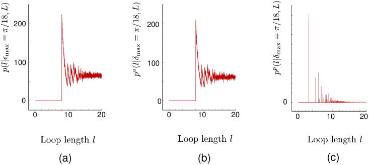
FIG. 14.: Loop length distributions $p(\epsilon_{\rm max}=\pi/16|L)$ for self-crossings (a) and $p^{a}(\delta_{\rm max}=\pi/16|L)$ for antiparallel avoided crossings; both practically coincide. Very different looking loop length distribution $p^{p}(\delta_{\rm max}=\pi/16|L)$ for parallel avoided crossings in (c) exhibits peaks near periodic orbit lengths since narrow parallel avoided crossings create loops close to periodic orbits; see Fig. 13 (e) and (40).

VII Symbolic dynamics for crossings and avoided crossings

A Crossings

We here propose to reveal how self-intersections with small angles and narrowly avoided crossings are reflected in symbolic words. That correspondence will lead us to some exact results for the Hadamard-Gutzwiller model, as well as a better understanding of the analytic-continuation relationship of crossings and avoided crossings. The ideas to be presented may also become important for generalizations of the Sieber-Richter theory to other models such as billiards, quantum graphs and maps.

In what follows, symbol sequences with brackets $\{...\}$ refer to periodic orbits, whereas sequences without brackets refer to parts thereof. Consider a crossing with angle $\epsilon$ dividing a periodic orbit into two loops. The symbolic word of the orbit will also be divided by the crossing into two parts which refer to a loop each and will be denoted by $A=a_{1}a_{2}\ldots a_{n_{a}}$ and $B=b_{1}b_{2}\ldots b_{n_{b}}$ where $a_{i},b_{k}$ are symbols from 0 to 7; see Fig. 15. The word of the whole orbit will be $\{AB\}=\{a_{1}a_{2}\ldots a_{n_{a}}b_{1}b_{2}\ldots b_{n_{b}}\}$, with the number of symbols $n=n_{a}+n_{b}$ and the length equal to the sum of the loop lengths, $L_{AB}=l_{A}(\epsilon)+l_{B}(\epsilon)$. The word is assumed pruned (see Section IV).

We recall that the loops $A,B$ can be continuously deformed to periodic orbits $\{A\},\{B\}$, whose lengths $L_{A},L_{B}\,$ related to the lengths of the loops by (25), i.e., as $\cosh\frac{l_{W}(\epsilon)}{2}=\cosh\frac{L_{W}}{2}/\sin\frac{\epsilon}{2}$ for ${\cal W}={\cal A}\mbox{ or }{\cal B}$; we shall also have to relate the lengths of both orbits to the traces of the corresponding Möbius-transformation matrices according to (6), i.e. $\cosh\frac{L_{W}}{2}=|\mathrm{Tr}\ \frac{{\mathcal{W}}}{2}|$. Here ${\mathcal{A},B}$ are the $2\times 2$ matrices obtained by taking the product of elementary matrices (7), in the order given by the symbol sequences $A,B$; the foregoing expression for $L_{W}$ also holds for non-regular octagons, with the elementary matrices (7) replaced by the pertinent generators.

FIG. 15.: Schematic decomposition of self-crossing orbit in segments, one per symbol. First letter $a_{1}$ of word $W$ and its part $A$ refers to one of two segments involved in crossing; similarly, first letter $b_{1}$ of $B$ refers to other crossing segment.

Summing up the loop lengths we get

$$L_{AB}=2\ \mathrm{arcosh}\left|\mathrm{Tr}\ \frac{{\mathcal{A}}{\cal B}}{2}\right|=2\ \mathrm{arcosh}\left|\frac{\mathrm{Tr\ {\mathcal{A}}}/2}{\sin\epsilon/2}\right|+2\ \mathrm{arcosh}\left|\frac{\mathrm{Tr\ {\mathcal{B}}}/2}{\sin\epsilon/2}\right|\,,$$ (42)

and, solving for $\sin^{2}\epsilon/2$

$$\sin^{2}\frac{\epsilon}{2}=\frac{(\rm{Tr}\ {\mathcal{A}B})(\rm{Tr}\ {\cal A})(\rm{Tr}\ {\cal B})-(\rm{Tr\ {\cal A}})^{2}-(\rm{Tr\ {\cal B}})^{2}}{(\rm{Tr\ {\cal AB}})^{2}-4}\equiv F({\cal A},{\cal B})\,,$$ (43)

except that the elementary derivation yields the first term in the numerator of the second member as $|({\rm Tr}\ {\mathcal{A}B})({\rm Tr}\ {\cal A})({\rm Tr}\ {\cal B})|$. We have, somewhat frivolously, dropped the modulus operation since numerical evidence suggests $(\rm{Tr}\ {\mathcal{A}B})(\rm{Tr}\ {\cal A})(\rm{Tr}\ {\cal B})\geq 0$ whenever the loops $A,B$ arise from a crossing; we regret not having found a proof, all the more so since only the form conjectured in (43) allows for analytic continuation to the case of avoided crossings (see below). Incidentally, the foregoing symbolic-dynamics expression for the crossing angle is the previously announced variant of the elementary-geometry result (35). For long orbits and loops we may approximate (43) as

$$\sin^{2}\frac{\epsilon}{2}\approx\frac{\mathrm{Tr}{\mathcal{A}}\ \mathrm{Tr}{\mathcal{B}}}{\mathrm{Tr}{\mathcal{A}B}}\,.$$ (44)

Inasmuch as a crossing is connected with the loops $A,B$, the right hand side of (43) must obey $0<F\,({\mathcal{A}},{\mathcal{B}})<1$. As regards the inverse statement, one must be a little careful. There can be several divisions of the word $W$ into parts $A$, $B$ leading to exactly the same value of $F(\mathcal{A},\mathcal{B})$. In this situation, the orbit has one and only one crossing with the angle defined by (43) (provided $0<F\,({\mathcal{A}},{\mathcal{B}})<1$), and only one of the divisions mentioned actually describes the loops associated to the crossing.

As an important application of the foregoing relation between crossing angles and symbolic words we can now find the condition on the word for the crossing angle to be small. As obvious from (44) we must have $\mathrm{Tr}{\mathcal{A}}\mathrm{Tr}{\mathcal{B}}<<\mathrm{Tr}{\mathcal{A}B}$. A crude estimate of these traces can be obtained by recalling that the length of an ergodic orbit with the (pruned!) word $W$ is roughly proportional to the number $n_{W}$ of letters in the word, $L_{W}\sim n_{W}d_{L}$, where $d_{L}$ is the average length per symbol (close to 1.6 in the regular octagon; see section V). Combining with (6) we find that the trace of the Möbius transform ${\mathcal{W}}$ grows exponentially with $n_{W}$,

$$\mathrm{Tr}\ {\mathcal{W}}\sim e^{\,n_{W}d_{L}/2}.$$ (45)

If $A,B$ are by themselves pruned words we have for the traces in (44) $\mathrm{Tr}{\mathcal{A}}\sim\mbox{e}^{n_{A}d_{L}/2},\mathrm{Tr}{\mathcal{B}}\sim\mbox{e}^{n_{B}d_{L}/2},\quad\mathrm{Tr}{\mathcal{A}B}\sim\mbox{e}^{(n_{A}+n_{B})d_{L}/2}$ with the trivial conclusion $\sin^{2}\frac{\epsilon}{2}\sim 1$; the crossing angle will not be small then.

Suppose, however, that the matrices ${\mathcal{A}}$ and ${\mathcal{B}}$ possess the structure

$${\mathcal{A}}={\mathcal{Z}}_{1}{\mathcal{L}Z}_{1}^{-1},\quad{\mathcal{B}}={\mathcal{Z}}_{2}{\mathcal{R}Z}_{2}^{-1}$$ (46)

with ${\mathcal{L}},{\mathcal{R}}$ generic Möbius transforms while the “insertions ” ${\mathcal{Z}}_{1},{\mathcal{Z}}_{2}$ are products of $many$ elementary matrices. Obviously the insertions disappear from the traces of the matrices ${\mathcal{A}}$ and ${\mathcal{B}}$ since $\mathrm{Tr}\ {\mathcal{A}}\equiv\mathrm{Tr\,}{\mathcal{Z}}_{1}{\mathcal{L}Z}_{1}^{-1}=\mathrm{Tr}{\mathcal{L}}$ and similarly for ${\mathcal{B}}$; they do not cancel in the trace of the product of ${\mathcal{A}B}$, however. Denoting ${\mathcal{Z}=Z}_{1}^{-1}{\mathcal{Z}}_{2}$ we have from (44)

$$\sin^{2}\frac{\epsilon}{2}\approx\frac{\mathrm{Tr}{\mathcal{L}}\ \mathrm{Tr}{\mathcal{R}}}{\mathrm{Tr}{\mathcal{L}ZRZ}^{-1\,\ }},$$ (47)

and can thus approximate the crossing angle as

$$\sin^{2}\frac{\epsilon}{2}\approx\frac{\epsilon^{2}}{4}\sim\mbox{e}^{-n_{Z}\,d_{L}},\quad n_{Z}\equiv n_{Z_{1}}+n_{Z_{2}}.$$ (48)

Very long insertions ${\mathcal{Z}}_{1},{\mathcal{Z}}_{2}$ will therefore yield very small crossing angles.

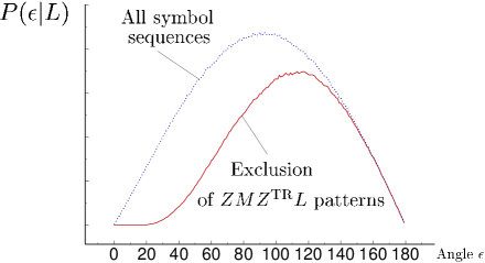
FIG. 16.: Self-crossing distribution $P(\epsilon|L)$ for ergodic orbits, and for subset of ergodic orbits with patterns $ZMZ^{\rm TR}L$ excluded. $All$ small-angle self-crossings disappear for latter subset.

To understand the physics behind condition (46) we recall from Section II that inverting a Möbius matrix means time reversal for the corresponding code; and that the time reverse of the code $Z=z_{1}\ldots z_{n}$ is $Z^{\mathrm{TR}}=\bar{z}_{n}\ldots\bar{z}_{1}$ with $\bar{z}=(z+4){\rm\mbox{ }mod\mbox{ }}8$. Condition (46) for the Möbius matrices therefore means

$$A=Z_{1}LZ_{1}^{\mathrm{TR}},\quad B=Z_{2}RZ_{2}^{\mathrm{TR}}\,.$$ (49)

The code of the total orbit can be written as $\{LZRZ^{\rm{TR}}\}$, with $Z=Z_{1}^{\rm{TR}}Z_{2}\,$. The shorter periodic orbits associated with the loops will have the codes $\{L\}$ and $\{R\}$. Since cyclic permutation is allowed in the code of orbits (not in loops!), the insertions can be brought together to form the self-canceling sequences $Z_{1}Z_{1}^{\mathrm{TR}}$ in $\{A\}$ and $Z_{2}Z_{2}^{\mathrm{TR}}$ in $\{B\}$. Using the locality of the code-to-trajectory connection (see Section III) we may say, somewhat loosely, that the loop $A$ is obtained by smoothly joining the periodic orbit $\{L\}$ with two pieces of trajectory, one visiting the boundaries of the octagon according to $Z_{1}$, and the other, encoded by $Z_{1}^{\mathrm{TR}}$, running through the same sequence of boundaries in the opposite direction. Such is precisely the behavior of a loop with a small crossing angle: The sections in the vicinity of the crossing nearly coincide up to the sense of traversal.

The loop structure (49) seems in fact necessary to produce a small crossing angle. Indeed, the beginning and ending parts of a loop being “nearly parallel” near a small-angle crossing the corresponding symbol sequences cannot help being locally identical, apart from time reversal. Impressive numerical evidence for the equivalence is provided by Fig. 16: Depicted are the densities $P(\epsilon|L)$ of crossing angles for a large generic set of symbol sequences and the subset purged of sequences of the indicated type; in the latter case no crossings with small angles are present.

B Avoided crossings

The symbolic dynamics of the avoided crossings is investigated in much the same way. One has to replace the loop length (25) by the corresponding results (37) and (38). That replacement suggests an interpretation as the analytical continuation $\varepsilon\rightarrow i\delta$ and $\varepsilon\rightarrow\pi+i\delta$ for antiparallel and parallel avoided crossings, respectively. The width of an avoided crossing dividing the orbit into the loops $A,B$ becomes

$$\sinh^{2}\frac{\delta}{2\,} = -F({\mathcal{A},B)}\approx-\frac{\mathrm{Tr}{\mathcal{A}}\ \mathrm{Tr}{\mathcal{B}}}{\mathrm{Tr}{\mathcal{A}B}}\ \ \ \ \mbox{ antiparallel ,}$$ (50)

$$\cosh^{2}\frac{\delta}{2\,} = +F({\mathcal{A},B)}\approx+\frac{\mathrm{Tr}{\mathcal{A}}\ \mathrm{Tr}{\mathcal{B}}}{\mathrm{Tr}{\mathcal{A}B}}\ \ \ \ \mbox{ parallel}\,,$$ (51)

where the approximate equalities refer to long orbits and loops, as in (44). It is obviously necessary that $F({\mathcal{A},B})<0$  ($F({\mathcal{A},B})>1)$  for the existence of an antiparallel (resp. parallel) avoided crossing. The width of the antiparallel avoided crossing will be small under the same assumptions (49) about the loops as in the case of small-angle crossings; the code of the whole orbit in both cases has the structure $LZRZ^{\mathrm{TR}}$ such that the distinction can be made only after calculating and thus determining the sign of $F({\mathcal{A},B)}$.

The Sieber-Richter theory is based on the fact that each orbit with a small crossing angle $\epsilon$ has a partner with almost the same length which avoids that crossing by the width $\delta\approx\epsilon$ (see the next subsection for precise relations between the loop lengths, $\epsilon$, and $\delta$); the partner has practically the same loops but one of them is traversed in the opposite sense relative to the original orbit. We can now translate these assertions into the language of symbolic dynamics. As we have just seen, a small-angle crossing divides the orbit into loops $A,B$ with the structure (49); consequently the partner must consist of the loops $A,B^{\mathrm{TR}}$. Accounting for long insertions near the crossing as after (49) we can state that each Sieber-Richter pair of orbits with small $\epsilon$ and $\delta$ must have codes $LZRZ^{\mathrm{TR}}$ and $LZR^{\mathrm{TR}}Z^{\mathrm{TR}}$. The crossing angle in one of the orbits and the closest-approach distance in its partner are defined by

$$\sin^{2}\varepsilon/2=F({\mathcal{L},ZRZ}^{-1}),\quad\sinh^{2}\delta/2=-F({\mathcal{L}}^{-1}{\mathcal{,}ZRZ}^{-1}).$$ (52)

Anticipating again $\epsilon\approx\delta\ll 1$ we conclude $F({\mathcal{L},ZRZ}^{-1})\approx-F({\mathcal{L}}^{-1}{\mathcal{,}ZRZ}^{-1})$ or, with the help of $\mathrm{Tr}{\mathcal{L}}=\mathrm{Tr}{\mathcal{L}}^{-1}$, $\;\mathrm{Tr}{\mathcal{L}ZRZ}^{-1}\approx-\mathrm{Tr}{\mathcal{L}}^{-1}{\mathcal{Z}RZ}^{-1}$. The approximate equality of the absolute values of the two traces is clearly necessary for the length of the two orbits in the pair to be close due to (6); the minus sign is less obvious.

C Crossing/avoided-crossing partnership

Even though we are mainly interested in pairs of orbits with small $\epsilon$ and $\delta$ it is interesting to further dwell on the crossing/avoided-crossing partnership for large angles and widths. We shall employ symbolic dynamics to rigorously relate the crossing angle $\epsilon$ to the closest-approach distance $\delta$ for such pairs and give exact expressions for the action difference in a pair and the distribution $P^{a}(\delta|L)$. Such results might be of importance for future investigations of higher-order terms in the expansion of the form factor.

We again imagine the symbolic code of an orbit bisected as $AB$; then the partner orbit with respect to that bisection will have the symbolic word $AB^{TR}$; the function $F({\cal A},{\cal B})$ defined in (43) will become $F({\cal A},{\cal B}^{-1})$ for the partner. As already indicated previously, numerical checks revealed the following behavior of $F$ under this replacement: (i) If the bisection $AB$ has $F({\cal A},{\cal B})>1$ the partner orbit $AB^{\rm TR}$ will also have $F({\cal A},{\cal B}^{-1})>1$; (ii) $F({\cal A},{\cal B})<0\;$ entails $\;0<F({\cal A},{\cal B}^{-1})<1$; (iii) finally, if $\;0<F({\cal A},{\cal B})<1\;$ then, the partner orbit has $F({\cal A},{\cal B}^{-1})<0$. If $A$ or $B$ contains less than $5$ symbols, and $F$ very close to 1, very rare exceptions to this rule occur.

Considering the previously established interpretations of the three cases (50), (51), and (43) we can say that partial time inversion of an orbit has the following respective consequences: (i) A parallel avoided crossing is replaced by another parallel avoided crossing; (ii) an antiparallel avoided crossing becomes a crossing in the partner; (iii) a crossing becomes an antiparallel avoided crossing in the partner. For very short loops with at most $5$ symbols and angles close to $\pi$ very rare exceptions occur.

We can use the last of these findings to more precisely define an antiparallel avoided crossing as the object emerging after the partial time reversal of some orbit $AB\to AB^{\rm TR}$  (or, equivalently, $AB\to A^{\rm TR}B$ ) provided the bisection $AB$ has a crossing according to $0<F({\cal A},{\cal B})<1$ while $F({\cal A},{\cal B}^{-1})<0$. As always, the word $AB$ is assumed pruned in the sense of Sect. III, i.e. written in the standard representation such that each of its letters indicates a side of the fundamental domain visited by the orbit. The code $AB^{\rm TR}$ of the partner orbit with an avoided crossing will then, however, not always be pruned, and the partner orbit will sometimes not have all its circular sections within the fundamental domain.

An example of a bisection of a pruned word for which partial time reversal yields a non-pruned word is provided by $A=LZ,\;B=RZ$. Then the symbolic word of the partner $AB^{\rm TR}=LZZ^{\rm TR}R^{\rm TR}$ obviously contains mutually canceling parts, and $LR^{TR}$ may become the standard encoding of an orbit in the fundamental domain. However, the avoided-crossing width in this case will be determined by the function $F({\cal LZ},{\cal Z}^{-1}{\cal R})$ in whose arguments the insertion ${\cal Z}$ may not be dropped. This situation occurs when the geodesic determining the width of the avoided crossing consists of several segments when depicted inside the octagon (see the preceding section). There is no reason not to take into account avoided crossings of the type just characterized. An orbit with an avoided crossing may thus contain fewer symbols and be appreciably shorter than its partner with a crossing. The closer the crossing angle is to $\pi$ the more often one meets with that situation.

According to our definition there is a one-to-one correspondence between crossings and avoided crossings. One might be tempted to infer that in each long ergodic orbit the number of crossings must be equal to the number of avoided crossings, but that temptation must be resisted. Given a fixed length $L$, there are fewer crossings than avoided crossings simply since by replacing a crossing with an avoided crossing one gets a shorter periodic orbit. Therefore, to obtain all avoided crossings with a certain width $\delta$ in the periodic orbits of length $L$ one has to make the crossing to avoided-crossing replacement in all orbits of length $L+\Delta L(\delta)$ with suitable length increments $\Delta L$, and longer orbits are more numerous due the exponential proliferation.

To find the relation between the density $P(\epsilon|L)$ of crossing angles and the density $P^{a}(\delta|L)$ of the avoided-crossing widths we write the total number of crossings in all periodic orbits with lengths in the interval $[L,L+dL]$ as $N(L)P(\epsilon|L)dLd\epsilon$ with Huber’s proliferation law $N(L)=\mbox{e}^{L}/L$. On the other hand, the number of avoided crossings with width $\delta$ in these orbits will equal the number of all crossings in the “parent” orbits whose lengths lie in $[L+\Delta L,L+\Delta L+dL]$ which is $N(L+\Delta L)P(\epsilon|L+\Delta L)dL|\frac{d\epsilon}{d\delta}|d\delta$. We may thus write

$$P^{a}(\delta|L)\approx\frac{\mbox{e}^{\Delta L}}{1+\frac{\Delta L}{L}}\ \left|\frac{d\epsilon}{d\delta}\right|\ P(\epsilon|L+\Delta L)\,,$$ (53)

where the approximate-equality sign again signals large $L$. It remains to determine the length shift $\Delta L(\delta)$ and the crossing angle $\epsilon(\delta)$, both as functions of $\delta$. Clearly, if we only wanted to find the ergodic part of $P^{a}(\delta|L)$ from $P_{\rm erg}(\epsilon|L)=(L^{2}/2\pi A)\sin\epsilon$ we could, in analogy with our procedure in Sect. V, drop the length shift $\Delta L$ everywhere in (53) except in the exponential proliferation factor; actually, we must be more ambitious and go for the next-to-leading order in $L$ as well since the latter is of relevance for the form factor.

To determine the functions $\mbox{e}^{\Delta L(\delta)}$ and $\epsilon(\delta)$ entering the foregoing expression we invoke two consequences of the definition (3) of $SU(1,1)$ matrices ${\cal A,B}$. First, we note ${\cal B}+{\cal B}^{-1}=\mathbf{1}\mbox{Tr }\cal{B}$ where $\mathbf{1}$ is the unit matrix. Second, on multiplying with $\cal A$ and taking the trace we get

$$\mbox{Tr}{\cal AB}+\mbox{Tr}{\cal AB}^{-1}=\mbox{Tr}{\cal A}\mbox{ Tr}\cal{B}\,.$$ (54)

Using the identity (54) we can rewrite the expressions (43) for the crossing angle and (50) for the avoided-crossing width as

$$\cos^{2}\frac{\epsilon}{2}=\frac{(\mbox{Tr}{\cal A})^{2}+(\mbox{Tr}{\cal A})^{2}-4-\mbox{Tr}{\cal AB}\mbox{ Tr}{\cal AB}^{-1}}{(\mbox{Tr}{\cal AB})^{2}-4}$$ (55)

$$\cosh^{2}\frac{\delta}{2}=\frac{(\mbox{Tr}{\cal A})^{2}+(\mbox{Tr}{\cal A})^{2}-4-\mbox{Tr}{\cal AB}\mbox{ Tr}{\cal AB}^{-1}}{(\mbox{Tr}{\cal AB}^{-1})^{2}-4}$$ (56)

and conclude

$$\frac{\cos^{2}\frac{\epsilon}{2}}{\cosh^{2}\frac{\delta}{2}}=\frac{(\mbox{Tr}{\cal AB}^{-1})^{2}-4}{(\mbox{Tr}{\cal AB})^{2}-4}\,.$$ (57)

Herein employing (6) and denoting the lengths of the periodic orbits with crossing and avoided crossing by $L_{\epsilon}$ and $L_{\delta}$ we proceed to

$$\frac{\cos\frac{\epsilon}{2}}{\cosh\frac{\delta}{2}}=\frac{\sinh\frac{L_{\delta}}{2}}{\sinh\frac{L_{\epsilon}}{2}}\,.$$ (58)

As by now familiar, slight simplifications arise in the physically interesting case of loops long enough for $\mbox{Tr}{\cal AB}$ to be much larger than both $\mbox{Tr}{\cal A}$ and $\mbox{Tr}{\cal B}$. The rigorous symbolic-dynamics expressions (55) for $\epsilon$ and $\delta$ then simplify to

$$\cos^{2}\frac{\epsilon}{2}\approx-\frac{\mbox{Tr }{\cal AB}^{-1}}{\mbox{Tr }{\cal AB}}\,,\;\;\;\;\cosh^{2}\frac{\delta}{2}\approx-\frac{\mbox{Tr }{\cal AB}}{\mbox{Tr }{\cal AB}^{-1}}$$ (59)

and yield the previously announced relation between the crossing angle in the parent orbit and the avoided crossing width in the partner,

$$\cosh\frac{\delta}{2}\approx\frac{1}{\cos\frac{\epsilon}{2}}\,,$$ (60)

which implies the familiar $\epsilon\approx\delta$ for small angles. Similarly, we may combine (58) and (59) to

$$-\frac{\mbox{Tr}{\cal AB}^{-1}}{\mbox{Tr}{\cal AB}}=\frac{\cosh\frac{L_{\delta}}{2}}{\cosh\frac{L_{\epsilon}}{2}}\approx\mbox{e}^{\frac{L_{\delta}-L_{\epsilon}}{2}}=\mbox{e}^{-\frac{\Delta L}{2}}$$ (61)

and thus get the length (and thus action) difference for an orbit with a self-crossing and its partner avoiding that crossing,

$$\Delta L\approx-4\ln\cos\frac{\epsilon}{2}=4\ln\cosh\frac{\delta}{2}\,;$$ (62)

the latter relation generalizes the result of Sieber and Richter [11, 12], $\Delta L=\epsilon^{2}/2$, to all orders in $\epsilon$.

An interesting geometric interpretation of our relations (62) between $\epsilon,\delta$, and $\Delta L$ in the framework of hyperbolic geometry will be presented in Appendix A. It may be well to once more say that the approximate-equality sign in these relations points to an error which is exponentially small when the loop lengths are large.

We can now write the factors converting the density of crossing angles into the density of avoided-crossing widths in (53),

$$\mbox{e}^{\Delta L}=\frac{1}{\cos^{4}\frac{\epsilon}{2}},\quad\frac{d\epsilon}{d\delta}=\frac{\tanh\frac{\delta}{2}}{\tanh\frac{\epsilon}{2}}\,.$$ (63)

The latter identities yield ${\rm e}^{\Delta L}|\frac{d\epsilon}{d\delta}|\,\sin\epsilon=\sinh\delta$ such that the ergodic angle distribution $P_{\rm erg}(\epsilon|L)=(L^{2}/2\pi A)\sin\epsilon$ yields the ergodic distribution of avoided-crossing widths $P_{\rm erg}^{a}(\delta|L)=(L^{2}/2\pi A)\sinh\delta$. Indulging in higher ambitions, we retain all terms of the next-to-leading (i.e. first) order w.r.t. to $L$ contributed by $(1+\frac{\Delta L}{L})^{-1}\,P(\epsilon|L+\Delta L)$ in (53). Taking the full angle density (30,34)

$$P(\epsilon|L)=\frac{L}{\pi A}\sin\epsilon\,\left(\frac{L}{2}-2\ln\frac{c}{2\sin\frac{\epsilon}{2}}\right)$$ (64)

from Sect. VI and using the above identities (63) to check $\Delta L-4\ln(c/2\sin\frac{\epsilon}{2})=-4\ln(c/2\sinh\frac{\delta}{2})$ we get

$$P^{a}(\delta|L)=\frac{L}{\pi A}\sinh\delta\,\left(\frac{L}{2}-2\ln\frac{c}{2\sinh\frac{\delta}{2}}\right)\,.$$ (65)

As a most welcome surprise, after combining all the ostensibly unrelated factors in (53), including those resulting from Huber’s exponential proliferation law, the final result is simply the analytical continuation of the crossing distribution to imaginary crossing angles.

D Example of a Sieber-Richter pair

In the previous subsection we have already commented on the symbolic codes for the periodic orbits in a Sieber-Richter pair as $\{AB\}$ and $\{A^{\rm TR}B\}$. To further clarify the role of symbolic dynamics for crossings, avoided crossings, and Sieber-Richter pairs we would like to present a concrete such pair in the regular octagon. Fig. 17 (a) displays a numerically found periodic orbit with a small-angle crossing. The reader is invited to read off the orbit segments, starting e.g. at the side 6 in the direction shown by arrows obtaining $6\to 3,\;7\rightarrow 6,\;2\rightarrow 6,\;2\rightarrow 4,\;0\rightarrow 5,\;1\rightarrow 2$ thus closing the loop. The starting side is always opposite to the landing side of the preceding segment, with their numbers differing by $\pm 4$. Hence it is sufficient to list the consecutive landing sides only: $\{\underline{3},6,\underline{6},4,5,2\}$. The sequence we got is the standard symbolic code of the orbit; the underlined symbols indicate the pair of segments crossing at the point $P$.

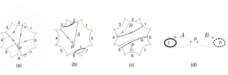
FIG. 17.: (a): Loops $A=3,6$ (full line) and $B=6,4,5,2$ (dashed) make up periodic orbit $AB=\{3,6,6,4,5,2\}$. (b): Periodic orbit L = $\{3,6\}$ (thick line) and loop A. (c): Periodic orbit $R=\{4,5\}$ (thick dashed line) and loop B. (d): Schematic picture of orbits $L,R$ and longer orbit $AB=\{LZRZ^{\rm TR}\}$ with crossing at point P obtained by deformation of $L$ and $R$.

The crossing $P$ divides the orbit into two loops shown by the full and dashed lines in Fig.17 (a); the symbol sequences of both loops $A=3,6$ and $B=6,4,5,2$ start with the symbol of the segment participating in the crossing. The periodic orbits associated with the loops and the loops themselves are shown by thick and thin lines respectively in Fig. 17(b) for loop $A$ and (c) for loop $B$. The periodic orbit $\{L\}$ associated with the loop $A$ has the same symbol sequence $\{3,6\}$ as the loop itself. The code of the orbit associated with the loop $B$ is shorter than that of the loop, namely, $\{R\}=\{4,5\}$ while $B=ZRZ^{{\rm TR}}$ with $Z=6$; of course, the insertions $Z$ fall out of the code of the loop-associated orbit. Inspection of part of Fig. 17(c) helps to appreciate insertions $Z$ in a loop like $B=ZRZ^{\rm TR}$ as due to the deformation of a circular segment of the periodic orbit $\{R\}$ overstepping the boundary of the octagon. Speaking pictorially we may say that the middle of the upper segment of $R$ was dragged upwards such that the vertex of the loop crossed the boundary 2 of the octagon, reappeared at the opposite boundary 6, and finally became the crossing point $P$, hence the insertions $Z=6$ and $Z^{TR}=2$. On the other hand, when deforming segment 3 of $L=3,6$ to the loop $A$ ( Fig. 17(c)) the octagon boundary is never reached, and therefore no new symbols appeared in the loop $A$ compared with the periodic orbit $\{A\}$.

To obtain the Sieber-Richter partner of the orbit $\{AB\}$ in Fig. 17 (a) we have to replace one of its loops, e.g. $A=3,6$ by its time reverse $A^{\rm TR}=\overline{6},\overline{3}=2,7$ . The partner periodic orbit thus formed $\{2,7,6,4,5,2\}$ is shown in Fig 18 (a) (dotted line) together with the original orbit (full line). The partner has an antiparallel avoided crossing whose width is approximately equal to the crossing angle in the original orbit; the relation valid to all orders in $\epsilon$ is given by (60). Note that apart from the two segments participating in the crossing (resp. avoided crossing) the two orbits run very close together; thus it is these two segments which contribute mainly to the difference in the orbit lengths.

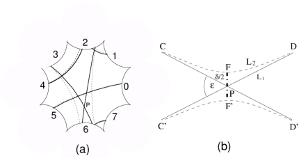
FIG. 18.: (a) Orbit of Fig. 17 with crossing at $P$ and partner avoiding that crossing. (b) Definition of crossing angle $\epsilon$ and avoided-crossing width $\delta$. When crossing/avoided crossing geometry (b) is folded into the fundamental domain $C$ is identified with $C^{\prime}$ and $D$ with $D^{\prime}$, and representation (a) results.

Financial support by the Sonderforschungsbereich ”Unordnung und große Fluktuationen” of the Deutsche Forschungsgemeinschaft is gratefully acknowledged. We have profited from discussions with Uwe Abresch, Ralf Aurich, Predrag Cvitanović, Gerhard Knieper, Christopher Manderfeld, Klaus Richter, Martin Sieber, Uzy Smilansky, Dominique Spehner, Frank Steiner, and Wen-ge Wang.

A Action difference for pairs from hyperbolic triangles

Consider a triangle $XYZ$ formed by geodesics on the pseudosphere, with the angles $X,Y,Z$ named after the respective vertices and the lengths of the respective opposite sides $x,y,z$. The following generalizations of elementary Euclidian-geometry relations hold true [6]

$$\cosh x=\frac{\cos Y\cos Z+\cos X}{\sin Y\sin Z},\quad\frac{\sin X}{\sinh x}=\frac{\sin Y}{\sinh y}=\frac{\sin Z}{\sinh z}\,.$$ (A1)

Let us apply these identities to the triangle $FPD$ in Fig. 18 (b) depicting the crossing and avoided crossing in a Sieber-Richter pair. Again naming the angles of the triangle after the respective vertices we have $F=\pi/2,P=\pi/2-\epsilon/2$. The point $D$ is supposed to be removed to infinity (recall the assumption of long orbits) such that the lengths $FD=L_{2}$ and $PD=L_{1}$ tend to infinity while the angle $D$ tends to zero. However, the difference $L_{2}-L_{1}$ remains finite and gives, up to an obvious factor 4, the length (or action) difference in search, $\Delta L=L_{\epsilon}-L_{\delta}=4(L_{1}-L_{2})$. From the first of the relations (A1) we get the connection between the crossing angle $\epsilon$ and the closest-approach distance $\delta=2FP$,

$$\cos\frac{\epsilon(\delta)}{2}\approx\frac{1}{\cosh\frac{\delta}{2}}\,,$$ (A2)

which we recognize as (60); similarly, the second group of relations in (A1) yields the length difference

$$\cos\frac{\epsilon}{2}=\frac{\sinh L_{1}}{\sinh L_{2}}\approx e^{L_{1}-L_{2}}\;\Longrightarrow\;\Delta L\approx 4\ln\cos\frac{\epsilon}{2}$$ (A3)

in agreement with (62). The association of symbolic dynamics and Möbius-transformation matrices employed in Sect. VII to derive the foregoing relations obviously incorporates the hyperbolic geometry of the Hadamard-Gutzwiller model.

B Effective number of symbols

We here determine the number $\nu(n)$ of non-equivalent $n$-letter words (alias periodic orbits with $n$ segments) $\gamma$ with an alphabet containing $p=8$ different letters. As mentioned in Section V, a rough estimate is $\nu(n)\approx(p-1)^{n}/n$, since a symbol $j$ may not be succeeded by its “inverse” $\bar{j}=(j+4){\rm\mbox{ }mod\mbox{ }}8$, and since a factor $1/n$ is due to the identification of cyclic permutations. The influence of the group identity

$$(0,5,2,7,4,1,6,3)=\mathbf{1}\,.$$ (B1)

requires more thought.

Our first task is to find the shortest possible version of a given word. Toward that end we note that whenever the sequence (B1) or any of its cyclic permutations is encountered within a word, we must delete that sequence and thus shorten the word by $8$ letters. Similarly, if some part of the identity with $m$ symbols and $4<m\leq 8$, is encountered, that part must be replaced by its complement with $8-m$ symbols. In any such instance the word is shortened by 8,6,4 or 2 letters. Next, we have to consider the $4$-symbol sequences for which the group identity provides an equivalent $4$-symbol sequence like for example $(0,5,2,7)=(7,2,5,0)$. If a word contains $k$ such 4-letter patches there are $2^{k}$ different representations of the same orbit; only one of these representations has the property that each symbol corresponds to one segment of the orbit inside the fundamental domain.

Let us start with the reversible 4-letter sequences and denote by $\alpha$ the probability that a symbol of a long word is the beginning of such a sequence. A combinatorial estimate of $\alpha$ can be made as follows. There are $16$ different $4$-letter patterns of the type in question, due to 8 cyclic permutations of both the identity in (B1) and its inverse, and each of these patterns occurs with probability $1/(8\times 7^{3})$. However, the pattern can only be included when the first and last letter are not the inverse of the neighboring one in the complete word, such that a ”junction factor” $(7/8)^{2}$ must be incorporated. The estimate in search thus comes out as $\alpha_{\rm comb}=(7/8)^{2}\times 16/(8\times 7^{3})\approx 0.00446$. Assuming independent occurrence of the 4-letter sequences we expect to find exactly $k$ of them in an $n$-letter word with the binomial probability

$$P_{n}(k,\alpha)=\frac{n!}{k!(n-k)!}\alpha^{k}(1-\alpha)^{n-k}\,.$$ (B2)

We refrain from attempts at improving that combinatorial estimate by accounting for the “interaction” of the 4-letter patches caused by their finite length. Upon checking many long words with randomly chosen letters we found such interaction effects quite unimportant: The binomial distribution (B2) is borne out very well with $\alpha_{\rm num}=0.00425$.

Similarly, let $\beta$ be the probability to find, in any letter, the beginning of any of the previously discussed $m$-symbol patterns with $4<m\leq 8$ which has an equivalent shorter partner with $8-m$ symbols. Again assuming independence of several such events we get a binomial distribution $P_{n}(k,\beta)$ as before and the combinatorial estimate for $\beta$ is, again neglecting “interactions”, $\beta_{\rm theor}=(7/8)^{2}[16/(7\times 8^{7})+16/(7\times 8^{6})+16/(7\times 8^{5})+16/(7\times 8^{4})]=0.00074$. Here again, the interactions were checked to be unimportant by going through a large sample of random words. The numerical data for $P_{n}^{\rm num}(k)$ so obtained once more fit the binomial distribution, with $\beta_{\rm num}=0.000716$. .

We can finally put all pieces together. The number of $n$-letter words allowed after excluding $j{\bar{j}}$ sequences of symbols and accounting for the equivalence of cyclic permutations was seen to be $(p-1)^{n}/n$; only the fraction $(1-\beta)^{n}$ of these cannot be shortened by using the group identity, so we are down to $(1-\beta^{n})(p-1)^{n}/n$ words. Roughly $P_{n}(k,\alpha)(1-\beta)^{n}(p-1)^{n}/n$ of these, however, contain precisely $k$ sequences of four letters each of which comes in two equivalent pairs due to the group identity; to avoid overcounting we have to divide out the multiplicity $2^{k}$. Finally summing over $k$ we get the desired number of different $n$-letter words as

$$\nu(n) = \sum_{k}\frac{n!}{k!(n-k)!}\frac{1}{2^{k}}\alpha^{k}(1-\alpha)^{n-k}(1-\beta)^{n}(p-1)^{n}/n$$ (B3)

$$= \frac{1}{n}[(1-\alpha/2)(1-\beta)(p-1)]^{n}=\frac{1}{n}{\rm e}^{n\ln p_{\rm eff}}\,,$$ (B4)

$$p_{\rm eff} = (1-\alpha/2)(1-\beta)(p-1)=6.98\,.$$ (B5)

Interestingly, the effective number of symbols is not drastically reduced from $p=8-1=7$ by the group identity equation (9).

REFERENCES

- [1] J. Hadamard, J. de Maths. Pures et Appl. 4, 27 (1898)
- [2] M.C. Gutzwiller, Phys. Rev. Lett. 45, 150 (1980)
- [3] M.C. Gutzwiller, Chaos in Classical and Quantum Mechanics (Springer, New York, 1990)
- [4] N.L. Balazs, A. Voros, Phys. Rep. 143, 109 (1986)
- [5] R. Aurich, F. Steiner, Physica D 32, 451 (1988)
- [6] S. Stahl, The Poincaré Half-Plane (Jones and Bartlett Pub., London, 1993)
- [7] R. Aurich, F. Steiner, Physica D 82, 266 (1995)
- [8] O. Bohigas, M. J. Giannoni, C. Schmit, Phys. Rev. Lett, 52, 1 (1984)
- [9] M. V. Berry, Proc. R. Soc. Lond. A, 400, 299 (1985)
- [10] M.C. Gutzwiller, J. Math. Phys. 12, 343 (1971)
- [11] M. Sieber, talk given at the 7th Genter Symposium, Ein Gedi (2001)
- [12] M. Sieber, K. Richter, Physica Scripta, T90, 128 (2001)
- [13] F. Haake, Quantum Signatures of Chaos, 2nd edition (Springer, Berlin, 2000)
- [14] G. Berkolaiko, H. Schanz, R. S. Whitney, Phys. Rev. Lett. 88, 104101 (2002); arXiv:nlin.CD/0205014
-
[15]
S. Müller, Diplomarbeit, Essen (2001);
M. Turek, K. Richter, talk given at the 66th DPG Frühjahrstagung, Regensburg (2002) - [16] U. Abresch, priv. comm.
- [17] P. Cvitanović, R. Artuso, R. Mainieri, G. Tanner and G. Vattay, Classical and Quantum Chaos, www.nbi.dk/ChaosBook/, Niels Bohr Institute (Copenhagen 2001)
- [18] G. Knieper, priv. comm.; A. Katok, B. Hasselblatt, Modern Theory of Dynamical Systems, Cambridge University Press
- [19] P.A. Braun, F. Haake, S. Heusler, J. Phys. A 35, 1381 (2002)
- [20] J. H. Hannay, A. M. Ozorio de Almeida, J. Phys. A 17, 3429 (1984)