[Phys. Rev. E 65, 065201(R) (2002)]

Cusp-scaling behavior in fractal dimension of chaotic scattering

Abstract

A topological bifurcation in chaotic scattering is characterized by a sudden change in the topology of the infinite set of unstable periodic orbits embedded in the underlying chaotic invariant set. We uncover a scaling law for the fractal dimension of the chaotic set for such a bifurcation. Our analysis and numerical computations in both two- and three-degrees-of-freedom systems suggest a striking feature associated with these subtle bifurcations: the dimension typically exhibits a sharp, cusplike local minimum at the bifurcation.

The development of nonlinear dynamics has led to new understanding of important physical processes, such as chaotic scattering Chaos_focus ; PG:book . A scattering process is chaotic if it exhibits a sensitive dependence on initial conditions in the sense that, a small change in the input variables before the scattering can result in a large change in some output variables after the scattering. Apparently, in a scattering process, every physical trajectory is unbounded, but chaos arises because of a bounded chaotic set (chaotic saddle) in the scattering region where, for instance, the interaction between particles and potential occurs, as in a potential scattering system. Chaotic saddles are nonattracting and, dynamically, they lead to transient chaos Tel:1990 . Chaotic scattering is thus the physical manifestation of transient chaos in open Hamiltonian systems, which occurs in a variety of physical contexts Chaos_focus .

An issue of fundamental importance in the study of chaotic scattering is to understand how the scattering dynamics changes characteristically as a system parameter is varied. There are three distinct classes of bifurcations in chaotic scattering: (1) routes to chaotic scattering from regular scattering, (2) metamorphic bifurcations in which the chaotic saddle suddenly changes its characteristics, and (3) topological bifurcations in which the topology of the chaotic saddle changes. Routes to chaotic scattering have been well documented, including abrupt bifurcations BGO:1990 ; Lai:1999 and saddle-center bifurcation followed by a cascade of period-doubling bifurcations Ding:1990 . There have also been efforts to study metamorphic bifurcations in chaotic scattering, such as crisis LG:1994 . Topological bifurcations, characterized by topological changes in the subsets of infinite number of unstable periodic orbits (UPOs) embedded in the chaotic saddles, on the other hand, have not been well understood. One example of topological bifurcation is the massive bifurcation Ding:1991 . This type of bifurcations is subtle but it is expected to be important in high dimensions, as they can lead to distinct, physically observable scattering phenomena High_d_scattering . While there have been quantitative scaling results concerning both routes to chaotic scattering BGO:1990 ; Tel:1991 and metamorphic bifurcation LG:1994 , the understanding of topological bifurcations in chaotic scattering remains largely at the qualitative level Ding:1991 , particularly in high dimensions High_d_scattering .

In this paper, we present a scaling law for the fractal dimension of the chaotic saddle in a topological bifurcation that appears to be typical in both two- Ding:1991 and three-degrees-of-freedom (DOF) High_d_scattering Hamiltonian systems. We focus on the fractal dimension because of its importance in shaping physically measurable quantities such as scattering functions, and because of the fact that most analytic scaling results associated with various routes to chaotic scattering concern fractal dimension but, to our knowledge, there has been none in the context of topological bifurcations. Due to the subtlety of a topological bifurcation, obtaining quantitative scaling laws, even numerically, is highly nontrivial. To be concrete, we state our main result in the context of potential scattering, with the particle energy $E$ as the bifurcation parameter. Let $E_{c}$ be the critical energy value at which a topological bifurcation occurs in the sense that, a class of infinite number of UPOs is destroyed and replaced by another. The principal result of this paper is then that, near the topological bifurcation, the fractal dimension of the set of singularities in any scattering function (to be described below) scales with the energy in the following way:

$$D-D_{c}\sim|E-E_{c}|^{D_{c}},$$ (1)

where $D_{c}$ is the dimension value at the bifurcation point. The remarkable observation is that the dimension-versus-energy curve exhibits a cusplike minimum at the bifurcation. We establish Eq. (1) by a scaling argument, and we provide numerical verification using a class of 2-DOF scattering systems. We also argue that the scaling law should hold in 3-DOF systems. Our result is interesting, as it represents the first, general, quantitative scaling result for topological bifurcation of chaotic scattering.

To derive the scaling law (1), we first consider 2-DOF potential scattering systems. Our idealized, albeit representative, scattering system consists of three potential hills in the plane, as shown in Fig. 1. The heights $E_{1},E_{2}$, and $E_{3}$ of hills 1, 2, and 3 satisfy $E_{1},E_{2}>E_{3}$. Assume that hill 3 has a circularly symmetric, quadratic maximum, and that it is close to the line connecting hills 1 and 2 so that the angle $\theta$ in the triangle formed by the centers of all three hills is greater than $90^{o}$, as shown in Fig. 1(a). When the particle energy $E$ is slightly above $E_{3}$, a trapped particle can move back and forth between hills 1 and 2 following three different paths Ding:1990 : $h$, $i$, and $j$, as shown in Fig. 1(a). When the energy drops below $E_{3}$, the path with greater deflection by crossing near the center of hill 3, path $j$, is destroyed because of the appearance of a new forbidden region around the center of hill 3, and is replaced by two new paths $k$, between hills 1 and 3 and between hills 2 and 3, as shown in Fig. 1(b). For $E\approx E_{3}$, the UPOs that form the skeleton of the chaotic saddle are thus composed of sequences of paths $h,i,j$, and $k$. A topological bifurcation Ding:1991 occurs at $E_{c}=E_{3}$, at which the class of an infinite number of UPOs containing path $j$ is destroyed and replaced by another class of infinite number of UPOs that contain paths $k$.

Figure 1: A topological bifurcation in 2-DOF case: basic paths composing UPOs (a) before and (b) after the bifurcation.

We focus on a fractal dimension that is physically most relevant: the dimension $D$ of the set of singularities in a scattering function. Suppose that we launch particles toward the scatterer from a line outside the scattering region and measure a dynamical variable characterizing the outgoing particles after the scattering ($e.g.$, scattering angle), as a function of a variable characterizing the incoming particles before the scattering ($e.g.$, impact parameter). Due to chaos, such a scattering function typically contains an infinite number of singularities that constitute a fractal set, which is the set of intersecting points between the stable manifold of the chaotic saddle and the line Dimension_saddle . Dynamically, the fractal set of singularities is constructed by successive interactions of the particles with the potential hills. For example, consider the interval $s$ of the line corresponding to particles that are first deflected by hill 1, as shown in Fig. 2. Three subintervals of this interval are then deflected by the other hills, with gaps between them corresponding to particles that are scattered to infinity right after the first interaction with hill 1. When $E>E_{c}$, these three subintervals are defined by particles that go from hill 1 to hill 2 along paths $h$, $i$, and $j$, respectively, as shown in Fig. 2(a). When $E<E_{c}$, while two of the subintervals are still defined by particles that follow paths $h$ and $i$, the third one is now determined by particles that go from hill 1 to hill 3 and back to hill 1, following path $k$, as shown in Fig. 2(b). In the next step each one of the three surviving subintervals will split into three smaller subintervals, and so on. The splitting due to hill 3 is recorded at successive interactions with hills 1 and 2. This process defines a Cantor set with three linear scales corresponding to the factors by which the intervals are reduced in each step: $\alpha\approx s_{h}/s$, $\beta\approx s_{i}/s$, and $\gamma\approx s_{j}/s$ ($E>E_{c}$) or $\gamma\approx s_{k}/s$ ($E<E_{c}$), as shown in Fig. 2.

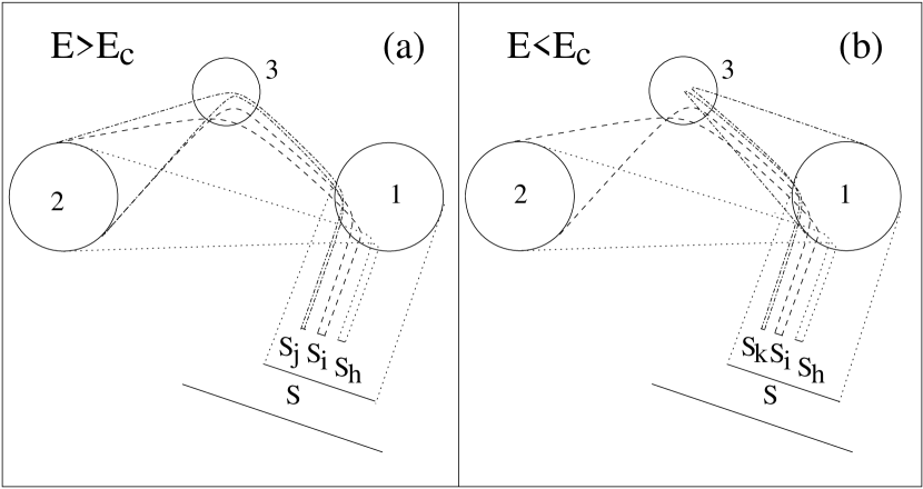
Figure 2: Construction of the Cantor set.

To obtain the dimension $D$ of the Cantor set, we employ the following scaling argument. Suppose that the critical energy $E_{c}$, the distance between the hills, and the effective radii of hills 1 and 2 at $E_{c}$ are of order unity. Near the bifurcation, the deflection angle $\phi$ due to hill 3 of the particles corresponding to the edges of the intervals $s_{j}$ and $s_{k}$, is smaller and greater than $90^{o}$ for $E\gtrsim E_{c}$ and $E\lesssim E_{c}$, respectively. In both cases, $|\tan{\phi}|$ is of order unity insofar as the angle $\theta$ is close neither to $90^{o}$ nor to $180^{o}$ so that $\tan(\pi-\theta)\sim{\mathcal{O}}(1)$ [see Figs. 1 and 2]. Thus, setting $|\tan{\phi}|$ to be of order unity provides an estimate of the width of the intervals $s_{j}$ and $s_{k}$, and hence an estimate of $\gamma$. For concreteness, say the maximum of the potential hill 3 (the bifurcation hill) has the following quadratic form: $V=E_{c}[1-(r/a)^{2}]$. A straightforward calculation One_hill indicates that if $|\tan\phi|\sim{\mathcal{O}}(1)$, then the impact parameter $b$ scales with the energy difference: $b\approx b_{0}|E-E_{c}|\equiv b_{0}\Delta$, where $b_{0}$ is proportional to $|\tan\phi|$. Therefore, the Cantor set is determined by the following scaling factors: $\alpha$, $\beta$, and $\gamma\approx\gamma_{0}\Delta$, where $\alpha$ and $\beta$ are constants, and $\gamma_{0}$ is constant on each side of the bifurcation. Under the approximation that there is a self-similarity in the fractal structure, the dimension $D$ satisfies the following transcendental equation BGO:1990 : $\alpha^{D}+\beta^{D}+\gamma_{0}^{D}\Delta^{D}=1.$ For $\Delta$ and $\delta\equiv D-D(E_{c})$ small, to the lowest order, this equation reduces to

$$[\Delta^{D(E_{c})}]^{\delta/D(E_{c})}=C\times\frac{\delta/D(E_{c})}{\Delta^{D(E_{c})}},$$ (2)

where $C$ is a positive constant. An asymptotic analysis of Eq. (2) leads to Solution our main scaling result (1) elliptical_hill .

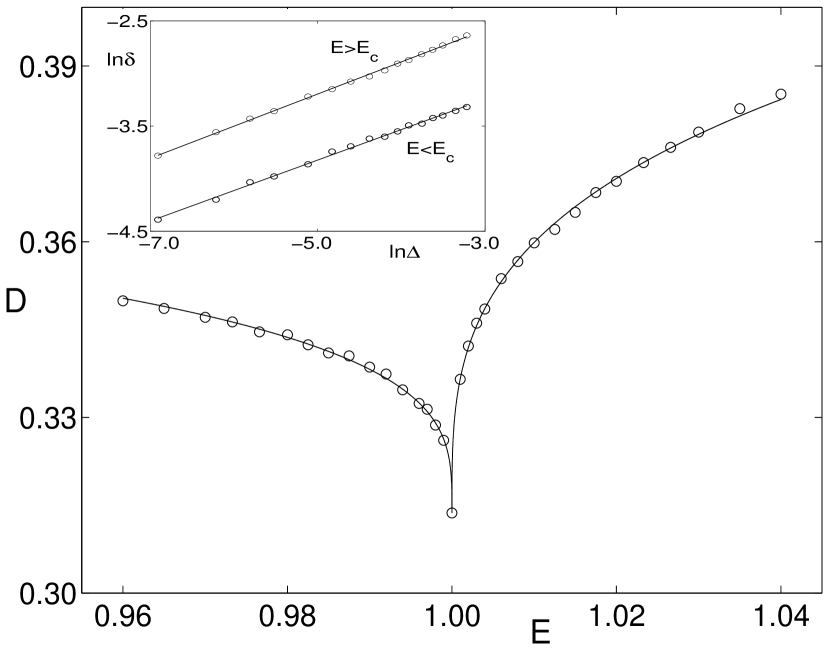
Figure 3: Numerically obtained cusp scaling behavior in the fractal dimension about a topological bifurcation.

We now present numerical confirmation for the scaling law (1). To resolve the cusp structure implied by Eq. (1) is a highly nontrivial task. For numerical feasibility we thus consider a planar scattering system consisting of three nonoverlapping potential hills located at the vertices ($x_{i},y_{i}$) ($i=1,2,3$) of an isosceles triangle Ding:1990 . Each potential is represented by the following function: $V_{i}(x,y)=E_{i}[1-(r_{i}/a_{i})^{2}]$ for $r_{i}\leq a_{i}$, where $r_{i}=\sqrt{(x-x_{i})^{2}+(y-y_{i})^{2}}$, and the potential is zero elsewhere. The Hamiltonian is thus: $H=|{\bf p}|^{2}/2m+V(x,y)$, where ${\bf p}$ is the two-dimensional momentum vector, and $V(x,y)=\sum_{i=1}^{3}V_{i}(x,y)$. The advantage of utilizing quadratic potential hills is that the motion of the particle inside each potential can be solved exactly, making a high-precision dimension calculation possible. In our numerical experiment, we choose the following set of parameter values: $E_{1}=E_{2}=10$, $E_{3}=1$, $a_{1}=a_{2}=2$, $a_{3}=1$, $(x_{1},y_{1})=-(x_{2},y_{2})=(4,0)$, $(x_{3},y_{3})=(0,2)$, and $m=1$. A topological bifurcation thus occurs at $E_{c}=1.0$. We utilize the uncertainty algorithm MGOY:1985 to compute the dimension $D$ of the set of singularities in scattering functions. For illustrative purpose, we choose the function to be the scattering angle to infinity $\psi\equiv\tan^{-1}{(p_{y}/p_{x})}$ versus the location of the upward (initially) particle on the horizontal line at $y_{0}=-4$. The result is shown in Fig. 3, in which the cusp behavior is unequivocal Computation . Linear least-squares fits between $\ln{[D(E)-D(E_{c})]}$ and $\ln{|E-E_{c}|}$ yield: $D(E)-D(E_{c})=(0.093\pm 0.005)\times(1-E)^{0.29\pm 0.03}$ for $E<E_{c}$ and $D(E)-D(E_{c})=(0.19\pm 0.01)\times(E-1)^{0.31\pm 0.03}$ for $E>E_{c}$, as shown by the inset in Fig. 3. The scaling exponents for both $E>E_{c}$ and $E<E_{c}$ agree well with the theoretically predicted one, the value of the dimension at $E_{c}$, which we obtain numerically: $D(E_{c})=0.314\pm 0.005$. In addition, the proportional factor in Eq. (1) is greater for $E>E_{c}$ than for $E<E_{c}$, which is also expected because, theoretically, this factor is proportional to $\gamma_{0}^{D(E_{c})}$ and $\gamma_{0}$ is greater in the former case. Overall, our computations lend strong credence to the validity of the scaling (1).

Our argument for the scaling law (1) can in fact be extended to chaotic scattering in 3-DOF Hamiltonian systems. As an example, we consider four potential hills but they are now located in the three-dimensional physical space at the vertices of a tetrahedron, as schematically illustrated by planar projection of the hills in Fig. 4(a) for $E>E_{c}$ and in Fig. 4(b) for $E<E_{c}$. We focus on the dimension $D$ of the intersecting set between the stable manifold of the chaotic saddle and a two-dimensional surface of the phase space, which is the dimension of the set of singularities in a scattering function on two variables. Arguments similar to those in the 2-DOF case can then be used to derive the scaling law (1) near a topological bifurcation, with the understanding that the dimension can in principle be either smaller or greater than 1. When the radii of the potential hills are small, $D(E_{c})<1$ can arise, in which case $dD(E)/dE$ diverges at $E_{c}$ and the dimension exhibits a cusp of the same nature as that in the 2-DOF case. If $D(E_{c})>1$, $dD(E)/dE$ goes continuously to zero as $E$ goes to $E_{c}$, which implies that the dimension should be smooth.

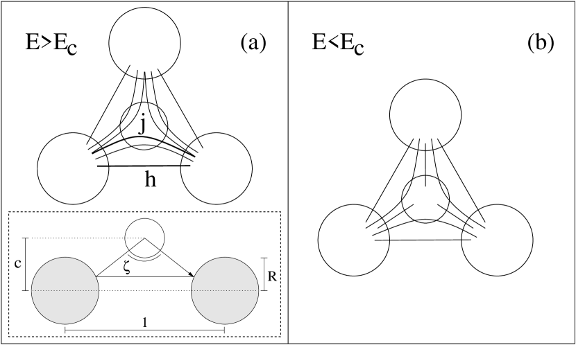
Figure 4: A topological bifurcation in 3-DOF case: basic paths (a) before and (b) after the bifurcation.

Can this smooth behavior be expected for a topological bifurcation in 3-DOF scattering systems? To obtain an answer, we note the defining characteristic of a topological bifurcation: the topology of the UPOs is changed but from the standpoint of symbolic dynamics, no symbol is missing. In our 3-DOF case it means that, before the bifurcation, all UPOs corresponding to periodic sequences of the nine basic paths shown in Fig. 4(a) must actually exist, while after the bifurcation, all those corresponding to sequences of the paths shown in Fig. 4(b) exist. In particular, the UPO represented by the sequence $\{h,j\}$ must exist when $E>E_{c}$. Without loss of generality, suppose that our 3-DOF system consists of three hard spheres of radius $R$ at the vertices of a regular triangle with edge of unit length, and a smooth bifurcation hill located on the symmetrical axis perpendicular to the center of the triangle. In the inset of Fig. 4(a) is shown the periodic orbit $\{h,j\}$ for $E>E_{c}$ in the limit $E\rightarrow E_{c}$. A necessary condition for the existence of this orbit, and hence for the occurrence of the topological bifurcation, is then $\zeta>90^{o}$ [see Fig. 4(a): the deflection angle due to hill 3 is smaller than $90^{o}$ when $E>E_{c}$]. In the three-dimensional physical space, however, there is an additional geometric constraint: $c>1/2\sqrt{3}$, where $c$ is the orthogonal distance from the center of the bifurcation hill to the lines connecting the hard spheres [Fig. 4(a)]. We obtain numerically that the conditions $c>1/2\sqrt{3}$ and $\zeta>90^{o}$ are satisfied simultaneously only for $R<0.39$. Numerical experiments indicate that, in this range of parameter values, $D(E_{c})$ is smaller than 1. It is reasonable to assume that the same is valid when the hard spheres are replaced by smooth potential hills. This implies that for a generic topological bifurcation in 3-DOF scattering systems, the cusp behavior in Eq. (1) is always expected Counter_example .

In summary, our scaling analysis and numerical computations reveal a striking behavior in the fractal dimension associated with topological bifurcations in chaotic scattering: the dimension typically exhibits a cusp as a function of the bifurcation parameter, with a local minimum at the bifurcation.

AEM was sponsored by FAPESP. YCL was supported by AFOSR under Grant No. F49620-98-1-0400 and by NSF under Grant No. PHY-9996454.

References

- (1) E. Ott and T. Tél, Chaos 3, 417 (1993), focus issue on chaotic scattering, and references therein.
- (2) P. Gaspard, Chaotic Scattering and Statistical Mechanics (Cambridge University Press, Cambridge, 1999).
- (3) T. Tél, in Directions in Chaos, edited by Bai-lin Hao (World Scientific, Singapore, 1990), Vol. 3.
- (4) S. Bleher, C. Grebogi, and E. Ott, Physica D 46, 87 (1990).
- (5) Y.-C. Lai, Phys. Rev. E 60, R6283 (1999).
- (6) M. Ding, C. Grebogi, E. Ott, and J. A. Yorke, Phys. Rev. A 42, 7025 (1990).
- (7) Y.-C. Lai and C. Grebogi, Phys. Rev. E 49, 3761 (1994).
- (8) M. Ding, C. Grebogi, E. Ott, and J. A. Yorke, Phys. Lett. A 153, 21 (1991); M. Ding, Phys. Rev. A 46, 6247 (1992).
- (9) A. E. Motter and P. S. Letelier, Phys. Lett. A 277, 18 (2000); Y.-C. Lai, A. P. S. de Moura, and C. Grebogi, Phys. Rev. E 62, 6421 (2000).
- (10) T. Tél, Phys. Rev. A 44, 1034 (1991).
- (11) The dimension is related to , the dimension of the chaotic saddle, as: .
- (12) The deflection angle due to a potential of the form satisfies , where is the impact parameter and is the initial distance to the center of the hill. For and it reads, . Therefore, implies , where .
- (13) Equation (2) has the following form: , where and . For , the asymptotic solution is , where is a constant. Clearly cannot be zero because if it were, then goes to zero much faster than does and, , which is inconsistent with the original equation. In fact, the consistence with Eq. (2) implies , from which follows and hence Eq. (1).
- (14) The scaling law (1) is valid for bifurcation hills with circularly symmetric maxima. The effect of asymmetric hill tops can be addressed by considering the situation where potential hill 3 has an elliptical maximum of the form , where Tel:1993 . In this case, we have and our analysis indicates that the corresponding scaling relation becomes . The dimension will thus display a cusp at insofar as .
- (15) T. Tél, C. Grebogi, and E. Ott, Chaos 3, 495 (1993).
- (16) S. W. McDonald, C. Grebogi, E. Ott, and J. A. Yorke, Physica D 17, 125 (1985); A. P. S. de Moura and C. Grebogi, Phys. Rev. Lett. 86, 2778 (2001).
- (17) To obtain Fig. 3, about 100 h of CPU time is required on a supercomputer consisting of 17 AMD 1.2 GHz CPUs.
- (18) The scaling relation (1) is derived for nondegenerate hills. An instructive counterexample can be constructed as follows. Take the planar scattering system in Fig. 1 and revolve it about the axis, which yields a 3-DOF system. The value of the dimension is increased by 1, leading to the following scaling relation: . The remarkable feature is that, despite , the cusp at is still present.