Dynamic Relationship between Diversity and Plasticity of Cell types in Multi-cellular State

Abstract

Dynamics maintaining diversity of cell types in a multi-cellular system are studied in relationship with the plasticity of cellular states. First, we introduce a new theoretical framework, reaction-diffusion system on ‘chemical species space’ to model intra-cellular chemical reaction dynamics. Then, by considering the cell division and death of such cells, developmental process from a single cell is studied. Cell differentiation process is found to occur through instability in transient dynamics and cell-cell interaction. In a long time behavior, extinction of multiple cells is repeated, which leads to itinerancy over successive quasi-stable multi-cellular states consisting of different types of cells. By defining the plasticity of a cellular state, it is shown that the plasticity of cells decreases before the large extinction, from which diversity and plasticity are recovered. After this switching, decrease of plasticity again occurs, leading to the next extinction of multiple cells. This cycle is repeated. Relevance of our results to the development, evolution is briefly discussed.

1 Introduction

In multi-cellular organisms, developmental process from a single cell or few homogeneous cells with multi-potency leads to an organism that consists of various cell types. Furthermore, in some multi-cellular organisms such as insects, the developmental process is generally accompanied by metamorphosis. There, several multi-cellular states are realized, which form quasi-stable distribution of cell types. In the event of metamorphosis, both the number of cells and the number of cell types decrease drastically, and then a different multi-cellular state is realized. In general, to consider the diversity of tissues in a multi-cellular organism, it is important to study how several stable distributions of different cell types are formed, sustained, or collapsed. What mechanism causes the transition between different quasi-stable states with several cell types? How is it related with the plasticity of cellular states?

As a theoretical framework for developmental process of multi-cellular organisms, “isologous diversification theory” is proposed by Kaneko, Yomo, and Furusawa[9, 10, 3, 4]. In these studies, dynamical systems approach is adopted, to show that robust developmental process with various cell types emerges based on the interplay between intra-cellular dynamics and inter-cellular interactions without finely tuned mechanisms. On the other hand, there are diversity at a tissue level, i.e., different stable distributions consisting of different cell types, in a usual multi-cellular organism. Switches among such quasi-stable multi-cellular states are also important. So far spontaneous formation of switches between several quasi-stable states is not much studied . In this paper, we study the dynamics to maintain the diversity of cell types and the emergence of switches among several quasi-stable multi-cellular states. Here all the cells change their states drastically in each switching accompanied by deaths of multiple cells. To quantify the switching mechanism, we define plasticity of a cellular state, as changeability of the state against external environmental change. As will be shown, the switching accompanied by multiple cell deaths is tightly related with the loss of plasticity.

As the development progresses, several cell types with low plasticity increase their number, which leads to extinction of multiple cell types, following the lack of chemical resources. Then a drastic change in environment is caused by the extinction, which leads to a large change of internal states of all the surviving cells. Then, different cell types with high plasticity are generated. From this ‘undifferentiated state’ as in the initial state, a new cell society with a different set of differentiated cell types is formed. This cycle is repeated.

For the purpose of the present study, we introduce a new modeling framework for internal chemical reaction dynamics, that is reaction-diffusion system on “chemical species space”. It can be regarded as an extended version of Boolean network model[12], so that each variable takes a continuous value. By adopting this modeling, one can correspond the dynamics of chemical concentrations with the fixed expression of genes, which is a common representation for each differentiated cell type. In this sense, the symbolic representation of cell types and differentiation rules are discussed from the dynamics, as is casted as the 5th problem in the open problem of Artificial Life[1]. We then discuss both the stability of realizing cell states and their diversity. We show that the above cycle to increase and decrease diversity and plasticity generally appears in our dynamical systems model.

In the next section, we describe the details of our model. After presenting the behavior of a single cell state in terms of the number of attractors in section III, developmental process is introduced in section IV. The condition to exhibit cell differentiation by cell-cell interaction and switching over several quasi-stable cell society is presented. In section V, we propose a feedback process leading to this switching, and confirm the relationship between the switching and the plasticity of total cells. Finally, in section VI, we briefly mention the generality of the present phenomenon and discuss the relevance to the development and evolution.

2 model

The basic strategy of the modeling follows the previous works[9, 10, 3, 4]. Our model consists of the following three parts:

• intra-cellular chemical reaction network

• cell-cell interaction

• cell division and cell death

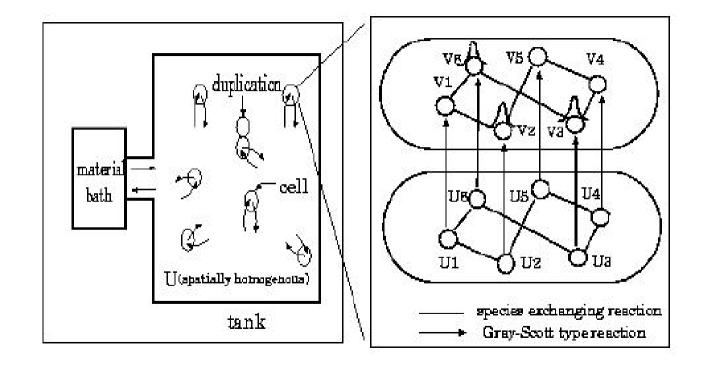
Figure 1: Schematic representation of our model.

Now we describe each process. In Fig.1, we show the schematic representation of our model.

• intra-cellular reaction network
  In general, intra-cellular chemical reactions consist of the reactions both of genes and metabolites. Genes are set to be on or off through the interactions between genes and metabolites. Genes and metabolites both compose reaction networks, while the time scale of reactions among genes are relatively slower than those of metabolites. Intra-cellular chemical reaction dynamics of our model is simply chosen and abstract so that it satisfies basic features described above.

  First, we assume a reaction network consisting of many products and resource chemicals similarly as that by genes and metabolites. The concentration of the $j$-th resources in $i$-th cell is denoted by $u_{i}^{j}(t)$ , while that of products is denoted by and $v_{i}^{j}(t)$. Here, product chemicals are synthesized autocatalytically by consuming corresponding resource chemicals. We adopt a variant of Gray-Scott model[5, 14] as this autocatalytic reaction scheme. . In this paper, we mainly present the results of the case where the number of members per each chemical is commonly set to $P=30$.

  Next we also assume species-exchanging reactions in each of product and resource chemicals, which form two random reaction networks. Each chemical is converted to other chemicals specified in reaction networks in proportion to the concentration difference between them. Here we adopt the same network for products and resources for simplicity, though it is plausible that these two networks are different from each other. It is noticed, however, that we also investigated models with different networks and obtained qualitatively the same results. The reaction network is represented by a reaction matrix $W{(i,j)}$, which takes 1 if there is a reaction from chemical $i$ to chemical $j$, and 0 otherwise. Here the reaction network is assumed to be symmetrical by considering reversible reaction, that is, if $W{(i,j)}$ takes 1, then $W{(j,i)}$ also takes 1. This network matrix is chosen randomly under the constraint of this symmetry while the number of reaction paths per each chemical is kept constant. The rate constant of species-exchanging reaction is set to $C$ in common with all resources, and $D$ in common with all products. Here we assume that $C$ is larger than $D$, by considering the difference in the time scales between genes and metabolites. These values are fixed throughout the simulation. Then, it is necessary to note that the system of random reaction network of species-exchanging reactions mentioned above is regarded as “diffusion” on random ‘chemical species space’, and with the reaction between products and resources, the intra-cellular reaction is regarded as a reaction-diffusion system. In that representation, each cell state corresponds to a discrete genetic expression pattern. We can realize multi-attractor states through bifurcations caused by the change of parameter $C$ or $D$.

  Since this model consists of the interacting gene network where all the gene expressions take continuous values, it includes both the concepts of Boolean network model[12] and reaction-diffusion system[16]. Thus, we can discuss both stability of each cell state and diversity of cell states.

• cell-cell interaction
  Assuming that environmental medium is completely stirred, we can neglect spatial variation of chemical concentrations in it, so that all the cells share the spatially homogeneous environment. Here we consider only the diffusion of some chemicals through the medium as a minimal form of interaction. In this model, we assume that only resource chemicals are transported through the membrane, in proportion to the concentration difference between the inside and the outside of a cell. All the resource chemicals have the same diffusion coefficient $D_{u}$. Each cell grows by taking resource chemicals from the medium and transforms them to product chemicals. $U^{j}$ is the concentration of $j$-th resources in the medium. Resource chemicals in the medium are consumed by cells, while we assume material bath outside of the medium and impose a flow of resource chemicals to the medium in proportion to the difference between the concentration in the bath and the medium. Again, all the resource chemicals have the same diffusion coefficient $D_{U}$ in the medium. The concentrations of all resources in the material bath, $U$ are set to be 1. The parameter $Vol$ is the volume ratio of a medium to a cell, and $N$ is the number of cells.

• cell division and cell death
  Each cell gets resource chemicals from the medium and grows by changing them to the product chemicals. When the total amount of product chemicals in a cell becomes twice the original, then the cell is assumed to divide, while if it is less than half the original, then the cell is put to death. In real biological system, cell division occurs after replication of DNA (which has smaller diffusion coefficient and cannot penetrate through the membrane). Hence these assumptions are rather natural. After cell division, each cell volume is set to be half. In cell division process, each cell is assumed to be divided into two almost equal cells, with some fluctuations. To be concrete, chemical concentration $a$($a$ is representation of $u$, $v$) is divided into $(1+\eta)a_{i}^{(j)}$ and $(1-\eta)a_{i}^{(j)}$ respectively, where $\eta$ is uniform random number over $[-10^{-3},10^{-3}]$. These fluctuations can give rise to a small variation among cell states, which eventually reaches to cell differentiation.

Accordingly, the concentration change of each chemical species is given by

$$du_{i}^{j}(t)/dt=D_{u}(U^{j}(t)-u_{i}^{j}(t))-u_{i}^{j}(t)v_{i}^{j}(t)^{2}+C\sum_{k=1}^{P}W{(j,k)}(u_{i}^{k}(t)-u_{i}^{j}(t))$$

$$dv_{i}^{j}(t)/dt=u_{i}^{j}(t)v_{i}^{j}(t)^{2}-Bv_{i}^{j}(t)+D\sum_{k=1}^{P}W{(j,k)}(v_{i}^{k}(t)-v_{i}^{j}(t))$$

$$dU^{j}(t)/dt=\frac{D_{u}}{Vol}\{\sum_{i=1}^{N}u_{i}^{j}(t)-U^{j}(t))+D_{U}(U-U^{j}(t))\}$$

In the model introduced above, a single cell has many fixed-point attractors, in contrast to the previous studies[9, 10, 3, 4], where a single cell can take one or a few attractors. The reasons why we adopt the present modeling are as follows. First many stable cellular states are realized in our model that allow for differentiations to many cell types. Second, as will be shown, by the instability through the interplay between transient states of cells and cell-cell interaction causes cell differentiations, although a single cell state eventually reaches fixed-point attractors after the transient time. Third, it is easy to classify cell types as different fixed point states, and is natural to relate them with different cellular states represented by different gene expressions.

3 Behavior of a single cell state

3.1 Initial conditions and methods

First we investigate the behavior of a single cell state without cell division and cell death. In all the simulations, we set the parameters $C=2.0$, $D=0.020$, $D_{u}=0.50$, $D_{U}=1.0$, $Vol=3.0$, $A=0.020$, $B=0.060$. These values of A$\sim$D correspond to typical values at which the original Gray-Scott model forms a self-replicating spot pattern in a one dimensional system. For numerical integrations, we used $\Delta t=0.010$ and $\Delta x=1.0$, while we have confirmed that the numerical results are qualitatively unchanged by using smaller values for $\Delta t$. We choose such initial condition that all the resource chemicals are 0.5 and all the product chemicals are randomly distributed in a cell. With this parameter setting, we get fixed point attractor for all cases.

3.2 Multiple attractors

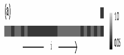
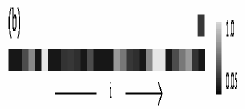
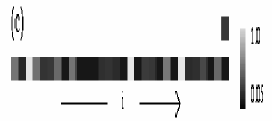
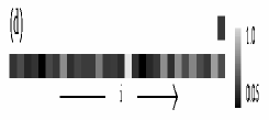
Figure 2: Examples of fixed point attractors. The concentrations of all the product chemicals for $i=1,2,\cdots,P=30$ are plotted with a gray scale. As the fixed point attractors, we adopt the state at $t=10000$. Four cases are studied, namely, one reaction path (a), two reaction paths (b), four reaction paths (c), and six reaction paths (d) per each chemical. Only one example is shown per each case.

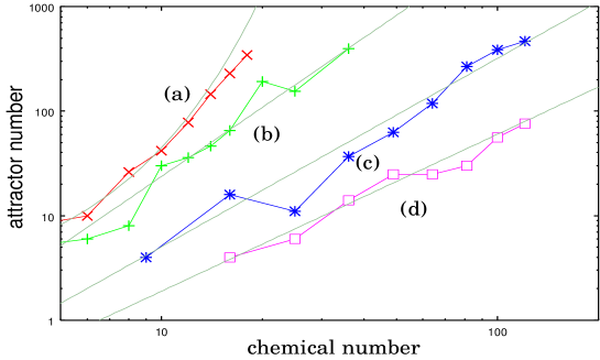
Figure 3: Dependence of the number of attractors on the number of chemicals $P$. Four cases are studied, namely, one reaction path (a), two reaction paths (b), four reaction paths (c), and six reaction paths (d) per each chemical. For each point of the figure, we take 500 different initial conditions with the use of only one reaction network. Numerically we check the state at $t=10000$ and classify the fixed-point attractors with the precision of $10^{-4}$.

Now we investigate how the number of attractor depends on the number of reaction paths per each chemical and the number of chemical species. The path number is varied from 1 to 6, and the number of chemical species $P$ is varied from 6 to 121. Examples of fixed point attractors for the cases with the path number 1(a), 2(b), 4(c), 6(d) with the number of chemicals $P=30$ are shown in Fig.2 using a gray scale for the concentration of product chemicals. All the attractors are fixed points, and can be distinguished easily. For each number of chemical species, we take one reaction network chosen arbitrary, and take 500 different initial conditions to count the number of attractors. Although we study only one reaction network for each, we can get the number dependence rather well, by carrying out simulations taking various values of $P$. The dependence of attractor number on $P$ is given in Fig.3.

As the number of species $P$ is increased, the number of attractors also increases, while as the number of reaction paths per each chemical increases, the number of attractors decreases. In case of one reaction path per each chemical, the reaction network is decomposed into $P/2$ pairs consisting of 2 chemicals, and each pair can take 2 states, so that the the number of attractors increases as $2^{P/2}$. In case of more reaction paths per each chemical, the the number of attractors increases with some power of $P$, that is larger than 1.

In Boolean network model, the number of attractor also increases with some power for 2 or 3 reaction paths per each chemical, with an exponent smaller than 1. Kauffman suggested that this relatively small number of attractors against the number of all genes suggests the stability of cell types in living systems[12]. We must point out, however, that all the states realized in Boolean network model are attractors of a single cell state. In fact, in real multi-cellular systems, cell states are not necessarily determined by possible stable states only of a single cell. It is often the case that cells take different states realized through cell-cell interaction[6]. It is rather plausible that such cellular states are selected that are stabilized through mutual relationship between intra-cellular dynamics and inter-cellular interaction. Hence we study multi-cellular states in the next section.

4 Developmental process with cell division and cell death

Now we discuss the change of cellular states under the process of cell division and cell death. Here the intra-cellular state and the inter-cellular interaction are mutually influenced. By cell-cell interaction, a homogeneous cell society of a single cell attractor may be destabilized, so that novel states may appear. We study such cell differentiation processes here.

4.1 Initial conditions and methods

First, we set an initial cellular state not exactly at an attractor of a single cell. If we start from an attractor of a single cell state, then the cells cannot differentiate by divisions any more. With the increase of cell numbers, all the cells compete for taking resources, and eventually they go to extinction. Once the state is on an attractor, the cell division gives two identical cells, as long as the fluctuation is not large to make a jump to different attractor. Here we simply adopt the initial condition of a single cell with $u_{i}^{j}(0)=0.50$ and $v_{i}^{j}(0)=0.250+0.01\times rand(j)$, where $j$ is natural number over [1,P] and $rand(j)$ is a uniform random variable over [-1,1].

Now we adopt two coarse-grained representations to analyze the cell differentiation events. The first one is introduced in order to distinguish cell types. We define a vector representation of each cell state denoted by $\overrightarrow{\rm X}$, where each element takes 0 or 1. This value is determined by the function given below and the concentration of each product chemical. All the cells that have the same $\overrightarrow{\rm X}$ are regarded to belong to the same cell type.

$\overrightarrow{\rm X}=F(\overrightarrow{\rm V})$, $\overrightarrow{\rm V}=(v^{1},v^{2},...,v^{(P)})$,

$F(Y)=\cases{1&($Y\geq 0.5$)\cr 0&($Y<0.5$)\cr}$

Second, to quantify the recursiveness of each cellular state, we compare the average concentrations of product chemicals in each cell between two successive division processes. $\overrightarrow{\rm V_{i}(n)}$ denotes the vector representation of the average concentration of all product chemicals in $i$-th cell between $n-1$th and $n$th cell division. $\overrightarrow{\rm X_{i}(n)}$ denotes a digital representation of $\overrightarrow{\rm V_{i}(n)}$, using the above threshold function $F(Y)$. As an index for the recursiveness of cellular state, we introduce an inner product denoted by $\theta_{i}(n)$ between $\overrightarrow{\rm X_{i}(n)}$ and $\overrightarrow{\rm X_{i}(n-1)}$. If $\theta_{i}(n)$ takes 1, the cell is regarded to keep the same type between successive cell divisions.

$\theta_{i}(n)=\frac{\overrightarrow{\rm X_{i}(n)}\cdot\overrightarrow{\rm X_{i}(n-1)}}{|\overrightarrow{\rm X_{i}(n)}||\overrightarrow{\rm X_{i}(n-1)}|}$, $\overrightarrow{\rm X_{i}(n)}=F(\overrightarrow{\rm V_{i}(n)})$,

$\overrightarrow{\rm V_{i}(n)}=(\overline{v_{i}^{1}},\overline{v_{i}^{2}},...,\overline{v_{i}^{(P)}})$, $F(Y)=\cases{1&($Y\geq 0.5$)\cr 0&($Y<0.5$)\cr}$

In this paper, each differentiated cell type is represented as distinctly separated chemical states of cells where each cell type can produce its own type recursively. We study the cell differentiation events with these two representations, by which we can distinguish a variety of cell states correctly.

4.2 The condition for cell differentiation

Here we study the frequency dependence of differentiation event on the structure of reaction network. As an index of network structure, we adopt the number of reaction paths per each chemical. We investigate four cases where the number of reaction paths per each chemical is 1(case (i)), 2(case (ii)), 3(case (iii)), 4(case (iv)) respectively. In each case, we take 100 different reaction networks, by taking a given initial condition. We carry out a simulation up to $t=20000$, to check the number of cells that exist exist at the moment, and the number of cell types. Here we note that if cell differentiation does not occur at all, all the cells go to extinction by the lack of resource chemicals. The other parameters and an initial condition are kept at the same values as previous section. The frequency of differentiation event for each case thus obtained is given in Fig.4.

Differentiation event occurs with highest probability in the case (ii). This is explained as follows:
In the case (i), transient time is shorter and the number of attractors is larger than the case (ii) in general. In each cell, all the chemicals cannot have global correlation among them but differentiate ‘selfishly’ by each cell, so that cooperative relations among cells to get resources effectively cannot be formed at a level of cell ensemble. As a result, the probability of extinction of all cells is high. On the other hand, in the case (iii) and (iv), transient time is shorter and the number of attractors is smaller than the case (ii) in general. In each cell, all the chemicals have rather strong global correlation among them. Hence it is difficult to amplify the small difference to reach cell differentiation, so that cooperative relations among cells to get resources cannot be well organized. As a result, the probability of extinction of all cells is again rather high. In the case of 5 or more reaction paths per each chemical, this tendency is observed more clearly. In case (ii), however, transient time is longest and the number of attractors is the second largest. In each cell, all the chemicals can have global correlation among them, and also can form cooperative relations among cells to get resources, so that cells can exist with maintaining cell differentiation for the longest period. Thus, differentiation events occur most probably at this intermediate number of paths.

4.3 Long time behavior of coexisting cell group

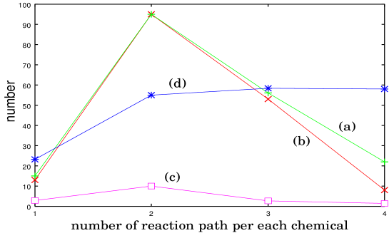
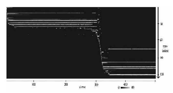
Figure 4: The frequency of cell differentiation plotted as a function of the number of the reaction paths per each chemical. We study the cases where the number of reaction paths per each chemical is ranged from 1 to 4. For each point of the figure, we take 100 different reaction networks and carry out a simulation up to $t=20000$ with the same initial condition and parameters mentioned in the text (without reaction network). Accordingly we plot the number of the event where cells exist without the whole extinction (a), the number of the event where cell differentiation occurs (b), the average number of cell types in the case with cell differentiation (c), and the average number of total cells in the case without the whole extinction (d).

Figure 5: An example of the long time behavior of cell differentiation process. Simulation is carried out up to $t=500000$ starting from a single cell, while the data for the total cells are sampled by every $1000$ time, to classify all cell types and to get the temporal change of population of each cell type. The initial condition and method for the classification of cell types are mentioned in the text. All cell types are shown in order of their appearance; a cell type that appears earlier in the simulation has a smaller index for the cell type. The population of each cell type is represented with a gray scale. Here the unit time of the figures is 1000.

Next we investigate the long time behavior of cell differentiation process. We adopt the case (ii), where the differentiation event is realized most clearly. We show an example of temporal evolution that is typically observed. Existing cell types and its population at every 1000 time are plotted in Fig.5. A multi-cellular cooperative state consisting of several cell types is formed in the beginning, and is maintained over a long period, which is much longer than typical transient time of single cell state. Then a sudden crisis occurs, and after some generations a new multi-cellular cooperative state with different cell types is recovered. This crisis is accompanied by the decrease of the cell number and diversity of cell types. This switching occurs generally, independent of the choice of the reaction networks.

5 Further Analysis of the switching process

5.1 methods for quantify the plasticity of cell types

Now we investigate the switching among several quasi-stable multi-cellular states in more details. Since the over all cell states are changed drastically in each switching, it is an effective way to study the process in terms of the temporal change of plasticity of cell types. Here we define the plasticity of each cell type as changeability of the cell state against environmental fluctuations, which are the change of concentrations of resource chemicals in the environment caused by cell divisions and deaths. To characterize the plasticity of cell state, we introduce the following quantity:
First we take $v_{i}^{j}(0)$, the concentration of $j$-th product chemical of the type $i$ cell, while we define $v_{i}^{j}(f)$ as the concentration of $j$-th product chemical of the attractor of the cell type $i$ when the assumptions of cell division and cell death are eliminated, to check the attractor state at the fixed environment. Then we define the “attractor distance” $Dist_{i}$ of the type $i$ cell, as the Euclid distance between $v_{i}^{j}(0)$ and $v_{i}^{j}(f)$, namely, $Dist_{i}=\sqrt{\sum_{j=1}^{P}{(v_{i}^{j}(f)-v_{i}^{j}(0))^{2}}}$.
As the distance is smaller, the cell type is closer to a specific attractor. Since the plasticity of a cell type is the changeability of the state by the environmental change, the plasticity is smaller as the state is close to a given attractor. We conjecture that the cell plasticity is characterized by the attractor distance, and the differentiation ability decreases as the attractor distance is smaller.

To confirm this conjecture, we have checked the following two relationships. First, the relation between the distance and the frequency of the occurrence of re-differentiation event when the a group of cells that consist only of the single cell type is chosen and is put to a new environment. The second is the relation between the distance and the degree of temporal fluctuations of each cell state when several cell types co-exist stably for a long term. If there are positive correlations in both cases, then the above conjecture is confirmed. These two relations are given in Fig.6 and Fig.7, for the data shown in the temporal evolution in Fig.5.

In Fig.6, we computed the attractor distances of all cell types that appeared in the temporal evolution, and divide the whole range of these attractor distances by 0.1 bin size, and measured the ratio of the occurrence of re-differentiation event for all the cell types belonging to each bin. (Here the population of each cell type is set to be 80. If the number is much larger, the homogeneous cell ensemble grown from the group goes to extinction by the lack of the resources. On the contrary, if the number is much smaller, then the effect to internal cell states caused by the change of the environment is so large that the difference of cell types cannot be well distinguished. Hence we choose this medium number for cell population.) The result roughly shows sigmoidal function dependence, that is, there is a threshold for the attractor distance below which the corresponding cell type loses the ability of re-differentiation drastically. This result also supports the initial condition dependence of cell differentiation event mentioned previously.

In Fig.7, we computed the temporal fluctuation of each cell type for two ranges in the temporal evolution, namely, $t=150000\sim 250000$ and $t=380000\sim 480000$, where several cell types co-exist stably. We measured the temporal fluctuation of each cell type as the average of all the Euclid distances of chemical concentrations between at the starting time and at some time span later. Here we take the time span as $t=1000$, so that in both cases, temporal fluctuations are calculated from $100$ data samples. The result shows that the temporal fluctuations of the chemical concentrations of a cell type are smaller as the attractor distance gets smaller.

Hence, it is confirmed that the attractor distance introduced above is valid as a measure of plasticity of cell type.

5.2 Mechanism for switching through extinction of many cells

Now we discuss the switching with multiple cell deaths in relationship with the loss of plasticity. Our results are summarized by the following scenario: At each stage of given quasi-stable multicellular states, cell types with different degree of plasticity coexist. Then at each stage, cell types with relatively high plasticity (i.e., larger attractor distance) differentiate to other cell types with lower plasticity, so that the ratio of cell types with lower plasticity increase gradually. Then the sustained relation among cell types to cooperatively use chemical resource chemicals is destroyed, and extinction of many cell types is resulted. With this multiple deaths, drastic change of the composition of environmental resource chemicals is brought about, which is large enough to make re-differentiation of some of surviving cells from the low plasticity state to a new state with high plasticity. Then, including with novel cell types with high plasticity, a novel multi-cellular state is brought about allowing for cooperative use of resources. With this drastic change, a spontaneous switch to novel multi-cellular state is generated.

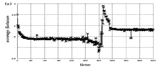
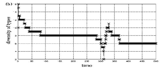
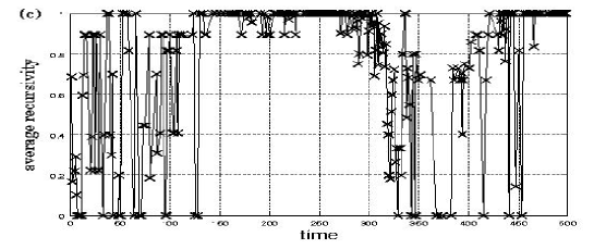
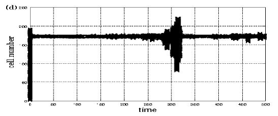
Figure 8: (a):The temporal change of the average attractor distance. (b):The temporal change of the average diversity over all cells. (c):The temporal change of the average recursiveness over cell types. (d):The temporal change of the total cell number. We computed all the quantities for the data given in the temporal evolution of Fig.5. Here the unit time of the figures is 1000.

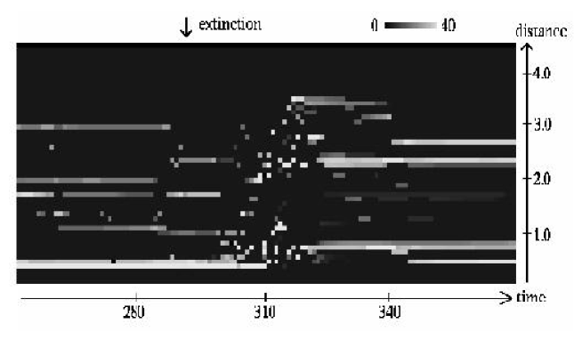
Figure 9: The temporal change of the population of existing cell types around the switching shown in Fig.5. The attractor distances of the cell types are plotted with their population. The time where the first extinction of many cells occurs is shown by the arrow. Here the unit time of the figures is 1000.

To verify this scenario, we computed the temporal change of the following four quantities in the temporal evolution of Fig.5: the average attractor distance for total cells (a), the total diversity of cell types (b), the average recursiveness of cell types over all cells (c), and total number of cell (d). Here, the average attractor distance is obtained by averaging the attractor distance of each existing cell type with the weight of the population ratio. The average recursiveness is also computed as the average over cells whose division event occurs in each $t=1000$ period. They are plotted in Fig.8, while the population size for each cell type with given attractor distance is plotted in Fig.9, around the switching regime.

In Fig.8, as the average attractor distance (a) starts to decrease, and the diversity of cell types is decreased, while the recursiveness is increased with strong fluctuations, until the attractor distance and diversity take the plateau with low values, when almost complete recursive production is sustained. After slight decrease of the first two values then, they go up to large values, with the multiple cell deaths and switching. After recovering the high plasticity and diversity, they again decrease to smaller values gradually. This process is repeated at each switching event. The data of Fig.9 also show the accumulation of population to cell types with low plasticity before the extinction, and recovery of the types with high plasticity after it. Although we show only one example here, the qualitatively same behavior is generally observed at each switching in our system. Hence, the scenario mentioned above is quantitatively demonstrated.

6 Summary and discussion

In this paper, we have studied a dynamical systems model of developmental process, by introducing a new framework, namely, reaction-diffusion system on ‘chemical species space’ for modeling internal chemical reaction networks. This modeling bridges between the two approaches: One is reaction-diffusion system proposed by Turing[16] and the other is Boolean network model proposed by Kauffman[12]. By further including the developmental process, states with many differentiated cell types are obtained, where the differentiation process to increase the diversity is observed. The condition to realize cell differentiation by cell-cell interaction is obtained. When the number of reaction paths per each chemical is larger than 2, all the chemicals are correlated strongly and the probability of realizing cell differentiation is lower. To the contrary, when the number of reaction paths per each chemical is 1, then all the chemicals cannot correlate enough and the probability of realizing cell differentiation is again lower. Cell differentiation occurs most probably when the number of reaction paths per each chemical is 2, that is, in the intermediate region above two cases. These results can be related with those obtained in the NKCS model by Kauffman[13].

In the long time behavior, we have found the switching over multi-cellular states that maintain diverse cell types. In each multi-cellular state, diverse cell types coexist to use chemical resources cooperatively, while the switching is characterized by multiple cell deaths arising from the loss of diversity of cell types, and the destruction of the cooperative use of the resources. This switching behavior is first observed in our model.

Then we propose that this switching behavior is characterized by the loss of plasticity of total cells, that is a general consequence of our dynamical systems theory. In each developmental stage, the irreversible loss of plasticity is a general course of the development, i.e., differentiation from a cell type with relatively high plasticity to that with lower plasticity, so that the ratio of cell types with lower plasticity increase gradually. Then the sustained relationship among cell types for cooperative use of resource chemicals is destroyed, which can cause multiple cell deaths. Then, drastic change of the composition of environmental resource chemicals is resulted, which allows for the change of surviving cell types from fixed states with low plasticity to new states with high plasticity. As a results, new multi-cellular state with novel cell types is generated. This process is repeated.

This give a feedback process in a system with many degrees of freedom to maintain the diversity of cell types, as has also been discussed as homeochaos[7, 8]. The plasticity of each cell type in our study corresponds to the mutation rate of each species in the study of homeochaos.

The existence of several quasi-stable multi-cellular states is important to consider the origin of tissues in multi-cellular organisms. In multi-cellular organisms, several tissues coexist that are represented as a different distribution of different cell types, consisting of cells with the same gene set. The switching of the states will be important to study how the life cycle of a multi-cellular organism is formed. In future, the search for a rule of transitions between successive multi-cellular states will be important. The dynamics of metamorphosis will be discussed along the line.

The present results are also relevant to study the evolution. As evolutionary processes, punctuated equilibria[2] are proposed, while extinction events after long quasi-stationary are also discussed. Successive extinction events of many cells may be extended to study evolution through extinctions. Here it is interesting to note that the distribution of the life-time of quasi-stable multi-cellular states in our model follows the power law distribution.

On the other hand, the inclusion of genetic mutations to our model is relevant to study speciation process to multiple species. Indeed, a theory of sympatric speciation with using phenotypic plasticity is recent proposed[11, 15]. In the preliminary studies of our model including genetic mutation process, we have observed sympatric speciation process to form several species, while with this process, the plasticity of each species defined in this paper decreases. Here, the recovery of plasticity of species after extinction of many cells is important to study open-ended evolution.

We would like to thank T.Yomo and C.Furusawa for stimulating discussions. This work is supported by Grants-in-Aid for Scientific Research from the Ministry of Education, Science and Culture of Japan (11CE2006, Komaba Complex Systems Life Project, and 11837004).

Figure 6: The relation between the attractor distance and the possibility of the re-differentiation. We compute attractor distance of all the cell types appeared in the temporal evolution shown in Fig.5. We take an ensemble of cells whose members have the same initial condition, and each cell is put it to a new environment and see whether cell differentiation occurs or not. By sampling the data for the attractor distance by 0.1 bin size, we compute the average ratio of the occurrence of re-differentiation event for each bin, to get the relationship between the differentiation ratio and the attractor distance.

Figure 7: Relation between the attractor distance and degree of temporal fluctuations of cell states. We calculate a temporal fluctuation of each cell type in two ranges in the temporal evolution shown in Fig.5, namely, $t=150000\sim 250000$ and $t=380000\sim 480000$, where several cell types co-exist stably. Temporal fluctuation of each cell type is computed as the average of all the Euclid distances between the starting state and the others. Here we take the data per $t=1000$.

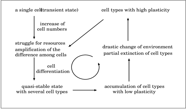
Figure 10: Schematic representation of our scenario for the mechanism to keep the diversity of cell types.

References

- [1] Bedau, M. A., McCaskill, J. S., Packard, N. H., Rasmussen, S., Adami, C., Green, D. G., Ikegami, T., Kaneko, K. Ray, T. S. (2000) “Open Problems in Artificial Life,” Artificial Life 6 363-376.
- [2] Eldredge, N., Gould, S. J. (1972) “Punctuated equilibria: The tempo and mode of evolution reconsidered,” in Modells in Paleobiology(ed. Schopf, T. J. M.), Freeman.
- [3] Furusawa, C., Kaneko, K. (1998) “Emergence of rules in cell society: Differentiation, hierarchy, and stability,” Bull. Math. Biol. 60 659-687.
- [4] Furusawa, C., Kaneko, K. (1998) “Emergence of multicellular organisms with dynamic differentiation and spatial pattern,” Artificial Life 4 79-93.
- [5] Gray, P., Scott, S. K. (1984) “Autocatalitic reactions in isothermal, continuous stirred tank reactor: oscillations and instabilities in the system A+2B3B,BC,” Chem. Eng. Sci. 39 1087-1097.
- [6] Gurdon, J. B., Lemaire, P. Kato, K. (1993) “Community effects and related phenomena in development,” Cell 75 831-834.
- [7] Ikegami, T., Kaneko, K. (1992) “Evolution of host-parasitoid network through homeochaotic dynamics,” Chaos 2 397-408.
- [8] Kaneko, K., Ikegami, T. (1992) “Homeochaos: Dynamics stability of symbiotic network with population dynamics and evoluving mutation rates,” Physica D 56 406-429.
- [9] Kaneko, K., Yomo, T. (1997) “Isologous diversification: A theory of cell differentiation,” Bull. Math. Biol. 59 139-196.
- [10] Kaneko, K., Yomo, T. (1999) “Isologous diversification for robust development of cell society,” J. Theor. Biol. 199 243-256.
- [11] Kaneko, K., Yomo, T. (2000) “Sympatric speciation: Compliance with phenotype diversification from a single genotype,” Proc. Roy. Soc. B 267 2367-2373.
- [12] Kauffman, S. A. (1969) “Metabolic stability and epigenesis in randomly constructed genetic nets,” J. Theor. Biol. 22 437-467.
- [13] Kauffman, S. A., Johnsen, S. (1991) “Coevolution to the edge of chaos: Coupled fitness landscapes, poised states, and coevolutionary avalanches,”J. Theor. Biol. 22 467-505.
- [14] Pearson, J. E. (1993) “Complex patterns in a simple System,” Science 261 189-192.
- [15] Takagi, H., Kaneko, K. Yomo, T. (2000) “Evolution of genetic code through isologous diversification of cellular states” Artificial Life 6 283-305;
- [16] Turing, A. M. (1952) “The chemical basis of morphogenesis,” Phil. Trans. Roy. Soc. B 237 37-72.