Transition from Gaussian-orthogonal to Gaussian-unitary ensemble in a microwave billiard with threefold symmetry

Abstract

Recently it has been shown that time-reversal invariant systems with discrete symmetries may display in certain irreducible subspaces spectral statistics corresponding to the Gaussian unitary ensemble (GUE) rather than to the expected orthogonal one (GOE). A Kramers type degeneracy is predicted in such situations. We present results for a microwave billiard with a threefold rotational symmetry and with the option to display or break a reflection symmetry. This allows us to observe the change from GOE to GUE statistics for one subset of levels. Since it was not possible to separate the three subspectra reliably, the number variances for the superimposed spectra were studied. The experimental results are compared with a theoretical and numerical study considering the effects of level splitting and level loss.

I Introduction

It is generally accepted that the eigenvalues of systems, whose classical counterparts are fully chaotic, behave similarly to those of random matrix ensembles Cas80 ; Boh84b . This conjecture also has some theoretical foundations Ber85 ; Ley92 ; And96 . If we disregard spin there are two random matrix ensembles, with two different behaviors under time reversal. Systems with time reversal invariance (TRI) are described by an ensemble of real symmetric matrices, corresponding to the invariance of the Hamiltonian under complex conjugation. This ensemble is known as the Gaussian Orthogonal Ensemble (GOE) and should be contrasted with the ensemble of all Hermitian matrices, known as the Gaussian Unitary Ensemble (GUE), which usually applies when TRI is broken.

An additional issue arises if discrete symmetries are present. In this case, it has been assumed that eigenvalues belonging to different irreducible representations of the symmetry group are statistically independent and obey GOE or GUE spectral statistics, depending on whether TRI holds or not. These assumptions have received considerable support both from theoretical considerations and from numerical simulations. However, in recent papers Ley96b ; Ley96a , it was suggested that an anomalous situation arises when a time-reversal invariant system has a discrete symmetry, such that TRI is broken within one of the irreducible subspaces of the point group. This is equivalent to the fact that the symmetry group has non-selfconjugate representations. In this case, TRI induces a degeneracy between different (conjugate) irreducible representations of the symmetry group (Kramers degeneracy). It was suggested that the eigenvalues belonging to these degenerate subspaces should have the statistical properties of the GUE rather than the GOE. This might be expected from the fact that complex conjugation actually maps one irreducible representation onto the other, rather than leaving it invariant. In this sense, one may indeed argue that TRI is violated within the subspace belonging to either representation, and is only restored through the combined presence of both representations. A more complete argument is presented in Ley96a . A semi-classical view of this question is given in Kea97 . At this point we should add a note of caution. This entire argument applies to the largest symmetry group of the system, and relies on the fact that this group is known. Deviations from the expectations would indicate the presence of a larger unknown symmetry group. On the other hand, symmetry breaking, which is usually present in experiment, will also affect the results. In the present paper we will address both points in a simplest example.

Let us now consider a system with threefold symmetry but with no twofold symmetry axis, i. e. $C_{3}$ symmetry. This means that the wave functions in polar coordinates can be put in the form

$$\psi_{n,\sigma}(r,\phi)=\sum_{k=-\infty}^{\infty}\phi_{k,n}(r)e^{i(3k+\sigma)\phi}\,,$$ (1)

where $n$ runs over all the integers and $\sigma$ takes the values $0$ and $\pm 1$. Because of TRI, it is clear that the eigenvalues corresponding to $\psi_{n,1}$ and $\psi_{n,-1}$ are degenerate, and we expect them to show GUE statistics. If in addition there is a twofold symmetry axis leading to $C_{3v}$ symmetry, the two conjugate representations combine to a two-dimensional irreducible representation which is self-conjugate. Thus we expect GOE statistics as well as degeneracy.

There is one previous microwave experiment on a billiard with $C_{3}$ symmetry performed by the Richter group Dem00b . In the data analysis the authors faced the problem to separate the subspectra belonging to different irreducible representations. Since it is impossible to realize a $C_{3}$ symmetry exactly in experiment, the doubly degenerate eigenvalues belonging to the $\sigma=\pm 1$ representations are split into doublets. In Ref. Dem00b this doublet splitting was used as a tool to separate the subspectra by classifying each pair of eigenvalues with a distance smaller than some given threshold value as a split doublet. The technique worked quite well, but there was a misidentification of about 5 percent of the levels. Nevertheless, the authors were able to see the GOE and GUE signatures in the respective subspectra. To improve the agreement with random matrix predictions, the authors calculated the spectrum numerically and used the results of the calculation to relabel the misidentified eigenvalues.

In the present work a billiard with threefold symmetry is studied, which has the additional feature to allow a change of symmetry from $C_{3v}$ to $C_{3}$ by turning an insert placed in the center of the billiard, thus allowing to study the transition from GOE to GUE behavior of the $\sigma=\pm 1$ subspectra. In view of the problems to separate the respective subspectra satisfactorily, we refrained from any attempt in this direction. Instead we concentrated on the spectral statistics for the superimposed spectrum and compared the results with numerical and analytic calculations based on random matrix theory (RMT).

A formula for the number variance is derived assuming that the degeneracy is lifted by a random off-diagonal matrix element between the two states of the doublets. It describes fairly well the long range properties of the spectra completed by means of level dynamics. The spectral short range behavior is sensitive to the details of the completion procedure while the long range behavior is not. This is why the difference between the GUE and the GOE case can still be detected very reliably in the long range regime.

If we consider the individual spectra there is a loss of roughly 20% of the levels. The number variance of the uncompleted spectra were compared with numerical RMT simulations. Several ways to simulate the loss of levels have been applied, and in all cases the two symmetries remained distinguishable at a loss rate of 20%.

In the following section the experimental setup and the details of the data analysis are presented. Further the gradual transition from the $C_{3v}$ to the $C_{3}$ symmetry will be observed in the number variance of the experimental spectra. In section III the results for the completed spectra will be compared with calculations taking into account the break of the $C_{3}$ symmetry. Finally, in section IV we will discuss the results for individual spectra with missing levels; these will be complemented with numerical RMT simulations.

II Experimental technique

The main features of the experimental technique have been presented elsewhere Kuh00b . Therefore we concentrate on the aspects of relevance in the present context. Figure 1 shows a sketch of the billiard used in the experiment. The interior insert can be rotated versus the outer part thus allowing a spectral level dynamics measurement in dependence of the rotation angle $\phi$. To avoid a break of symmetry due to the presence of the antenna, three antennas were placed at symmetry equivalent positions, two of them being terminated by $50\,\Omega$ loads. Spectra were taken for angles from $\phi=0^{\circ}$, corresponding to the geometry with $C_{3v}$ symmetry shown in the figure, to $\phi=20^{\circ}$ in steps of one degree. All boundaries, both of the insert and the outer part, were curved, and the corners of the outer boundary were removed to avoid families of marginally stable orbits such as bouncing balls. This was checked by means of a Poincaré plot of the classical motion of a particle in the billiard.

Figure 1: Sketch of the microwave billiard used in the experiment at angle $\phi=0^{\circ}$. The positions of the antennas are marked by crosses.

The height of the billiard was $h=10$  mm, i. e. the system was quasi-two-dimensional for frequencies below $\nu_{\rm max}=c/2h=15$ GHz. Microwave reflection spectra were taken with a Wiltron 360B vector network analyzer in the frequency range 0.5 to 7 GHz with a resolution of 0.5 MHz. In the studied spectral range one expects to find altogether 400 eigenvalues for each angle $\phi$. This number is obtained from the Weyl formula with area and circumference term

$$\bar{n}(k)=\frac{A}{4\pi}k^{2}-\frac{S}{4\pi}k\,.$$ (2)

$\bar{n}(k)$ is the mean integrated density of states, where $A\approx 0.258$ m² and $S\approx 3.59$ m are area and circumference of the billiard, and $k=2\pi\nu/c$ is the wave number. The curvature of the billiard yields a correction term of the order of 1. The number of states identified for a fixed angle falls approximately 20% short of the Weyl estimate. It is possible to recover all missing eigenvalues by studying the dynamics of the spectra as a function of the angle. This is demonstrated in Fig. 2 where the positions of the missing resonances are marked by diamond-shaped symbols.

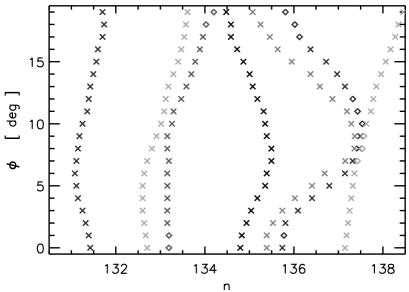
Figure 2: Part of the spectral level dynamics for the billiard with threefold symmetry with the orientation angle $\phi$ of the central insert as the level dynamics parameter. Angle $\phi=0^{\circ}$ corresponds to $C_{3v}$ symmetry. Only the resonances marked by cross-shaped symbols were really found in the experiment. At the positions marked by diamond-shaped symbols missing resonances were supplemented.

We begin with a presentation of the number variance in dependence of the insert angle, both for the completed and uncompleted spectra. In both cases the spectra were unfolded to a constant mean density of states using a second order polynomial fit to the experimental integrated density of states. The number variance $\Sigma^{2}(L)$ has been obtained by moving the interval of length $L$ through each spectrum on a fine grid to not loose any information. Consequently, the smoothness of $\Sigma^{2}(L)$ does not reflect its statistical quality, since the intervals are not statistically independent.

Figure 3 shows the number variance $\Sigma^{2}(L)$ for different angles $\phi$, where the results for $\phi=0^{\circ},1^{\circ}$, $\phi=2^{\circ},3^{\circ}$, $\phi=4^{\circ},5^{\circ}$ and $\phi=6^{\circ},7^{\circ}$ have been averaged. We see a gradual transition from the $C_{3v}$ to the $C_{3}$ case with increasing $\phi$. The line with long dashes shows an average over $\phi=8^{\circ}\ldots 19^{\circ}$, corresponding to the $C_{3}$ case. The GOE-GUE transition is clearly seen, both in the completed and the uncompleted spectra. In the following we will only discuss the two extreme cases, where for the $C_{3v}$ case the results for $\phi=0^{\circ},1^{\circ}$ will be averaged and for the $C_{3}$ case the ones for $\phi=8^{\circ}\ldots 19^{\circ}$.

Figure 3: Number variance $\Sigma^{2}(L)$ for different angles $\phi$ for the completed (a) and the uncompleted (b) spectra. The results for $\phi=0^{\circ},1^{\circ}$ (upper solid line), $\phi=2^{\circ},3^{\circ}$ (dashed), $\phi=4^{\circ},5^{\circ}$ (dash-dotted), $\phi=6^{\circ},7^{\circ}$ (dotted), were averaged. The lower solid line shows an average over $\phi=8^{\circ}\ldots 19^{\circ}$.

III Results for the completed spectra and the doublet splitting

We recall that for $\phi=0^{\circ}$ we expect a superposition of one GOE spectrum and another doubly degenerate GOE spectrum for the ideal system, whereas for angles $\phi$ sufficiently different from zero a superposition of one GOE spectrum with a doubly degenerate GUE spectrum should be observed. The short range behavior is dominated by doublet splitting, which we have no reliable experimental handle on. We therefore concentrate on the long range behavior. In particular we consider the long range part of the two-point correlation function. The number variance is ideally suited for this purpose because of the clear signature it shows for the difference between the GOE and the GUE case.

For the superposition of $M$ strictly non-interacting, equally weighted subspectra the number variance can be written as

$$\Sigma_{\rm{total}}^{2}(L)=\sum_{m=1}^{M}\Sigma_{m}^{2}\left(\textstyle{\frac{1}{M}}L\right)\,.$$

In the case of a threefold symmetry, the three subspectra are not independent; instead two of them are degenerate and thus the covariance of this doublet spectrum leads to a factor 2 in the number variance of their superposition:

$$\Sigma_{\rm{total}}^{2}(L)=\Sigma_{1}^{2}\left(\textstyle{\frac{1}{3}}L\right)+4\,\Sigma_{2}^{2}\left(\textstyle{\frac{1}{3}}L\right)\,.$$ (3)

Here $\Sigma_{1}^{2}$ is the number variance of the singlet spectrum being a GOE spectrum in both cases, whereas $\Sigma_{2}^{2}$ is the number variance of the doublet spectrum which may be a GOE or a GUE spectrum, depending on the symmetry of the system.

In the analysis of the completed spectra, the first 70 eigenvalues of each spectrum have been omitted to avoid non-generic features in the statistics. The results for the number variance of the experimental spectra have been averaged over the rotation angles $\phi=0,1^{\circ}$ in the $C_{3v}$ case and $\phi=8..19^{\circ}$ in the $C_{3}$ case. This implies that the statistical fluctuations of the number variance are much larger in the former case.

Figure 4 shows experimental data with solid lines for the $C_{3v}$ (a) and the $C_{3}$ (b) case, respectively, while the dotted lines give the ideal result of Eq. 3. It is not surprising that the agreement is poor, since we already noticed in the level dynamics that the doublet spectrum was rather strongly split, indicating a sizeable break of the $C_{3}$ symmetry of the billiard. On the other hand, we clearly see that the two number variances differ, and that the effect is quite large. This was the motivation for further theoretical considerations of the symmetry breaking. A detailed discussion of this issue follows in the appendix, where an expression for the corresponding number variance is derived. Here only the main points shall be outlined.

Figure 4: Number variance $\Sigma^{2}(L)$ of the completed spectra for the mirror-symmetric (a) and the non-mirror-symmetric (b) case. The experimental results (solid line) are compared with the theoretical prediction for the ideal system (dotted line), and with an analytical result, where the doublet splitting was taken into account (dash-dotted line).

The case of the $C_{3}$ symmetry is the more delicate one. The basis functions spanning the irreducible subspaces are complex, but due to the degeneracy we can always choose real functions. The appendix gives formal explanations, but here it may suffice to say that the actual measurements are on real fields and therefore it is clear that the smallest perturbation that does lift the degeneracy must cause real linear combinations. Therefore it is not surprising that we have to use degenerate perturbation theory for a real symmetric matrix. Furthermore it is quite clear that the perturbation matrix elements should be Gaussian distributed. While the mechanical imperfections causing the breakdown of the symmetry are the same for all functions, the unperturbed eigenfunctions involved are those of a chaotic system and thus in good approximation random functions that should yield Gaussian distributed matrix elements. Based on these simple considerations it is clear that the level splitting is Gaussian distributed, too, and linear in the perturbation. In the appendix we obtain an expression for the effect of such a level splitting on the long range part of the number variance, and we also show that effects of three level terms are small and thus effects of the symmetry breaking on the number variance for larger distances are of second order in the perturbation.

This result is of central importance since it explains why the difference in the number variances persists in spite of the fairly large doublet splitting. A parameter $\Delta=0.125$ for the width of the distribution of the perturbation matrix element and thus for the doublet splitting (see Eq. 8), is consistent with the splitting found in the experiment. It corresponds to a mean level splitting of about 0.85 in units of the mean level spacing. If we now use the results of the appendix for the number variance, Eq. 13, both for the GOE and the GUE case, we find good agreement with the experimental results, as can be inferred from the dash-dotted line in Fig. 4. The small deviations are consistent with the statistical uncertainties seen in skewness and excess (not shown). We therefore have a clear understanding of the role played by the splitting of the degeneracy and why it does not affect the difference between the two cases even if the symmetries are only approximate.

IV Missing levels and individual spectra

Completing the spectra by means of spectral level dynamics we were able to come to a quantitative theoretical understanding of the GOE-GUE transition observed in the experiment. The completion of spectra is definitely a legitimate approach, but in general only isolated spectra for fixed systems are available. Therefore we felt the need to check the robustness of the signatures of the transition by considering what we can learn from incomplete spectra with as many as 20% of the levels missing.

Numerical simulations have been performed as follows. We produced ensembles of 1000 spectra of dimension 500 to create the GOE or the GUE doublets for the $C_{3v}$ and $C_{3}$ case respectively. Then we lifted the degeneracy randomly using a Gaussian distribution with a width of about 12.5% of the average level distance of a single spectrum. These spectra have been superposed with an independent GOE spectrum of the same strength.

In the next step we tried to simulate the experimental loss. There are two sources of missing levels. First, close pairs can no longer be resolved if their separation is smaller than the line width. Second, a level will be missed if incidentally a node line of the associated wave function will be just at the position of the antenna. This mechanism leads to a loss that is uniformly distributed along the energy axis.

So we skipped randomly 7% of the eigenvalues to simulate the global loss due to the position of the antenna. Then we compared the distance between two adjacent levels with a Gaussian distributed random number whose width is chosen such that around 13% of the doublets are destroyed. From these spectra only 30% of the levels at the center of each spectrum are taken into account for the further analysis in order to avoid edge effects. The ratio of uncorrelated and correlated loss has been chosen to get a fair correspondence between experiment and theory for $\Sigma^{2}$ at small distances and is consistent with values found in previous works (see e. g. Ref. shu94 ).

The numerical as well as the experimental results for the nearest neighbor distribution for the case of $C_{3}$ symmetry are presented in Fig. 5. A good qualitative agreement between the two curves is found, although the first bins are underestimated in the numerical data resulting in an overshoot of its maximum. In Figure 6 the experimental results for both symmetries are compared with the numerics. In both cases we get a rough agreement up to $L=3$. For larger distances the slope of the numerical curve is by far too large which indicates that we have somehow destroyed long range correlations still present in the experimental data. On the other hand, the reliability of the experimental data for large $L$ is questionable because of the missing levels. Therefore it seems unreasonable to fit parameters like the percentages of the two sources of level missing. In any case, both the experimental results as well as the numerical calculations permit a clear distinction between the two symmetry cases.

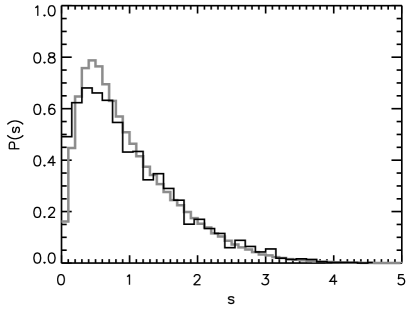
Figure 5: Nearest neighbor distribution for the case of $C_{3}$ symmetry. The black line shows the results for the experimental data with 20% loss, the grey line shows the numerical simulations.

Figure 6: Number variance $\Sigma^{2}(L)$ of the experimental data with 20% loss (solid line: $C_{3v}$, dash-dotted line: $C_{3}$ case) in comparison with the numerical simulations (dashed line: $C_{3v}$, dotted line: $C_{3}$ case).

V Conclusions

We have presented experimental results for a quasi-two-dimensional microwave cavity with a movable insert permitting to change the discrete symmetry of the cavity from $C_{3v}$ to $C_{3}$. According to theory, this change should modify the spectral statistics in the ideal case from a superposition of two GOE spectra, one of them degenerate, to a superposition of a GOE spectrum with a degenerate GUE spectrum. We find that the level splitting due to imperfections in the $C_{3}$ symmetry amounts to about 0.85 of the mean level spacing, and we face up to 20% loss of levels in an isolated spectrum. From spectral level dynamics by rotating the cavity’s insert we can recover the entire spectra, with some errors in the short range behavior of correlation functions. Nevertheless, the long range part of the number variance still clearly displays the difference between the two cases. From a theoretical analysis of the symmetry breaking in terms of degenerate perturbation theory, this behavior becomes comprehensible, since the level splitting is linear in the perturbation while long-range effects are quadratic.

Even more importantly, we have shown that the spectral statistics of spectra with large loss of levels can still provide usable information. By postulating two types of losses, a statistical one due to the fact that the antenna may be close to a node of the wavefunction and a systematic one due to overlap of close-lying levels, we can explain the experimental results qualitatively.

Appendix A Number Variance for perturbed $C_{3}$ symmetry

In this appendix we present a detailed treatment of the effect of symmetry breaking. We first need to specify a reasonable RMT model for this system. To this end let us consider an unperturbed Hamiltonian matrix $H_{0}$ representing the billiard with perfect $C_{3}$ symmetry. The Hilbert space can be separated into three irreducible parts, one invariant under the group action, the other two spanned by clockwise and counterclockwise travelling waves. Because of TRI the eigenfunctions in the latter two subspaces have pairwise degenerate eigenvalues, i. e. they display a Kramers degeneracy. If we wish to display TRI rather than the $C_{3}$ invariance we can alternatively use a real basis for the doublet space. Any perturbation due to imperfections of the billiard can only break the $C_{3}$ symmetry but not TRI. As we wish to introduce an RMT model for the perturbation that conserves TRI, it is obvious that this can be implemented by a real symmetric matrix in the real basis.

From this picture the effect of the perturbation is immediately clear: Since we have degenerate eigenvalues, we must look at these separately. Then we may ask what happens if there is a third eigenvalue in the vicinity. We therefore consider the matrix

$$A=\left(\matrix{0&V_{1}&V_{2}\cr V_{1}&0&V_{3}\cr V_{2}&V_{3}&1\cr}\right),$$ (4)

where we have scaled and shifted the two degenerate eigenvalues to zero, and the perturbing third eigenvalue one. The eigenvalues $\lambda_{i}$ obey the relations

$$\lambda_{1}+\lambda_{2}+\lambda_{3} = 1$$

$$\lambda_{1}^{2}+\lambda_{2}^{2}+\lambda_{3}^{2} = 1+2(V_{1}^{2}+V_{2}^{2}+V_{3}^{2})$$ (5)

$$\lambda_{1}\lambda_{2}\lambda_{3} = -V_{1}^{2}+2V_{1}V_{2}V_{3}\,.$$

These equations are satisfied to second order in the $V_{i}$ by

$$\lambda_{1} = V_{1}$$

$$\lambda_{2} = -V_{1}$$ (6)

$$\lambda_{3} = 1\,.$$

The shift in the two degenerate eigenvalues, being linear in the off-diagonal element $V_{1}$, thus dominates all other perturbations as long as the $V_{i}$ are small with respect to the third eigenvalue. If on the other hand the third eigenvalue is so close to the degenerate doublet that the $V_{i}$ are of the order of one, the situation becomes more complex and Cardan’s formula must be used. However, the splitting will still be linear in the $V_{i}$, so that the qualitative behavior should not be greatly affected. The probability for one doublet to come close to another one is very small, since they experience GUE level repulsion.

We now turn to the calculation of the spectral form factor, and of the number variance for a weakly split GUE doublet spectrum. Let us take the $\epsilon_{k}$ to be an arbitrary reference spectrum with mean level spacing equal to one. The split doublet spectrum is generated by

$$E_{k,\sigma}=2\epsilon_{k}+\sigma a_{k}\,,$$ (7)

where $\sigma$ runs over $\pm 1$ and the factor 2 retains the mean level spacing of one. The $a_{k}$ are taken to be independent Gaussian random variables distributed according to

$$p(a)=\sqrt{\frac{1}{2\pi\Delta}}\exp\left(-a^{2}/(2\Delta)\right).$$ (8)

We are now going to compute the form factor

$$k(t)=\frac{1}{2N}\sum_{\sigma,\sigma^{\prime}=\pm 1}\sum_{k,l=1}^{N}e^{2\pi i(E_{k,\sigma}-E_{l,\sigma^{\prime}})t}$$ (9)

from the corresponding quantity $k_{0}(t)$ for the $\epsilon_{k}$. Separating the right hand side into a part for $k=l$ and another for $k\neq l$ and averaging over the $a_{k}$ yields

$$k(t)=1+e^{-8\pi^{2}\Delta t^{2}}-2e^{-4\pi^{2}\Delta t^{2}}+2k_{0}(2t)e^{-4\pi^{2}\Delta t^{2}}\,.$$ (10)

The number variance $\Sigma^{2}(L)$ can be expressed as (see e. g. Ref. Ber88 )

$$\Sigma^{2}(L)=\frac{2}{\pi^{2}}\int_{0}^{\infty}dt\,k(t)\left(\frac{\sin\pi Lt}{t}\right)^{2}\,.$$ (11)

Thus, from Eq. 11 we get the $\Sigma^{2}_{d}(L)$ for the doublet part of the spectrum by inserting the GUE form factor

$$k_{0}(t) = |t|\qquad(|t|\leq 1)$$

$$= 1\qquad(|t|>1)$$

into (10). From this one finally obtains for the number variance of the superimposed spectrum

$$\Sigma^{2}_{total}(L)=\Sigma^{2}_{d}\left(\textstyle{\frac{2}{3}}L\right)+\Sigma^{2}_{1}\left(\textstyle{\frac{1}{3}}L\right)\,,$$ (13)

where $\Sigma^{2}_{1}(L)$ is the number variance of the GOE singlet spectrum.

The $C_{3v}$ case yields a similar result if we substitute the GOE form factor rather than the GUE form factor for $k_{0}$ in Eq. 10.

References

- (1) G. Casati, F. Valz-Gris, and I. Guarneri, Lett. Nuov. Cim. 28, 279 (1980).
- (2) O. Bohigas, M. Giannoni, and C. Schmit, Phys. Rev. Lett. 52, 1 (1984).
- (3) M. Berry, Proc. R. Soc. Lond. A 400, 229 (1985).
- (4) F. Leyvraz and T. Seligman, Phys. Lett. A 168, 348 (1992).
- (5) A. Andreev, O. Agam, B. Simons, and B. Altshuler, Phys. Rev. Lett. 76, 3947 (1996).
- (6) F. Leyvraz and T. Seligman, in Proceedings of the IV Wigner-Symposium in Guadalajara, Mexico, edited by N. Atakishiyev, T. Seligman, and K. Wolf (World Scientific, Singapore, 1996), p. 350.
- (7) F. Leyvraz, C. Schmit, and T. Seligman, J. Phys. A 29, L575 (1996).
- (8) J. Keating and J. Robbins, J. Phys. A 30, L177 (1997).
- (9) C. Dembowski et al., Phys. Rev. E 62, R4516 (2000).
- (10) U. Kuhl, E. Persson, M. Barth, and H.-J. Stöckmann, Eur. Phys. J. B 17, 253 (2000).
- (11) A. Shudo et al., Phys. Rev. E 49, 3748 (1994).
- (12) M. Berry, Nonlinearity 1, 399 (1988).