Chaotic stirring by a mesoscale surface-ocean flow

Abstract

The horizontal stirring properties of the flow in a region of the East-Australian Current are calculated. A surface velocity field derived from remotely sensed data, using the Maximum Cross Correlation method, is integrated to derive the distribution of the finite-time Lyapunov exponents. For the region studied (between latitudes 36^∘S and 41^∘S and longitudes 150^∘E and 156^∘E) the mean Lyapunov exponent during 1997 is estimated to be $\lambda_{\infty}=4\times 10^{-7}$ s^-1. This is in close agreement with the few other measurements of stirring rates in the surface ocean which are available. Recent theoretical results on the multifractal spectra of advected reactive tracers are applied to an analysis of a sea-surface temperature image of the study region. The spatial pattern seen in the image compares well with the pattern seen in an advected tracer with a first-order response to changes in surface forcing. The response timescale is estimated to be 20 days.

Satellite imagery of the ocean surface shows that sea-surface temperature and chlorophyll have complex distributions. The filaments and whorls characteristic of tracers in stirred fluids are often clearly evident. Despite the importance of stirring to a range of problems, such as plankton ecology, larval transport or predicting the fate of pollutants, it has not been well described. Here we analyse the stirring properties of a velocity dataset obtained from the interpretation of sequential satellite images. The finite-time Lyapunov exponents of the flow are determined. Using these results, we show that the patterns seen in a sea-surface temperature image are consistent with those formed from the advection of a reactive tracer. This suggests that an understanding of the distribution of tracers such as temperature and chlorophyll in the surface ocean must include a representation of both the chaotic advection by the flow and the dynamics of the tracers themselves. If the advection can be characterised, as we have been able to do here, then it may be possible to use the information contained in sea-surface imagery to infer the time-scales of the tracer dynamics.

I Introduction

One of the simplest measures of the distribution of a tracer is its power-spectrum, which quantifies the variability in the distribution at each spatial scale. Between inverse wavenumbers of $1$ and $100$ km the spectra of sea-surface temperature and chlorophyll are usually found to have a power-law form, $F(k)\sim k^{-\beta}$. The exponent, $\beta$, is typically in the range $1.5<\beta<2.5$ Gower et al. [1980], Deschamps et al. [1981], Denman and Abbott [1988], Ostrovskii [1995], Piontkovski et al. [1997], Washburn et al. [1998]. Where both sea-surface temperature and chlorophyll are measured at the same time their spectra often have similar slopes. Ocean currents are turbulent within the mesoscale wavenumber range, 1 km $<k^{-1}<$ 100 km, and their energy falls off rapidly at higher wavenumber Monin and Ozmidov [1985]. The flow within this range is approximately two dimensional, and it is appropriate to consider the advection of a passive tracer in the surface ocean as a stirring process Garrett [1983], Pierrehumbert [1994]. Stirring acts to stretch and fold patches of tracer, distorting them into long tendrils and filaments. In spectral terms, variance that is input at low wavenumber is transferred by stirring towards higher wave-numbers, where it is dissipated by diffusion. The spectrum of a stirred tracer, which has a source at low wavenumber but is otherwise conserved, is expected to be power-law with an exponent $\beta=1$ Batchelor [1959]. Batchelor law spectra with this form are sometimes seen in laboratory experiments of stirring by two-dimensional flows Wu et al. [1995], but $\beta=1$ is outside the range usually measured for sea-surface temperature and chlorophyll, as has been noted by several authors Gower et al. [1980], Deschamps et al. [1981]. It is clear, however, that neither sea-surface temperature or chlorophyll are conserved quantities. For a non-conserved tracer which satisfies a first-order equation, any spectral exponent $\beta>1$ can be obtained, depending on the relation between the reaction-rate and the typical stirring-rate of the flow Corrsin [1961]. This suggests that the patterns seen in the surface ocean may reflect both the stirring by the flow and the tracers’ non-conservation. Recently, results have been derived which give the multifractal structure of an advected reactive tracer in terms of the distribution of finite-time Lyapunov exponents, which characterise the stirring by the flow Neufeld et al. [2000]. The theoretical results were derived in the context of Lagrangian chaotic flows. Applying the theory to the surface ocean is hampered by the lack of data on stirring by ocean currents. The few measurements which have been made depend on following the stretching of a tracer patch for an extended period of time Ledwell et al. [1993, 1998], Abraham et al. [2000]. This technique gives little information on the distribution of stirring rates, each observation of a tracer patch typically returning only a single estimate of the stirring. Given the lack of direct measurents, an indirect approach must be taken. In this paper, surface velocity data, inferred from satellite observations, are used to calculate stirring rates. The analysis is focussed on the East Australian region, where there is strong mesoscale eddy activity and where a suitable dataset is available. The derived distribution of stirring rates, more formally finite-time Lyapunov exponents, is applied to an analysis of the distribution of sea-surface temperature.

II Surface velocity data

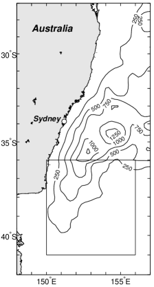
Figure 1: The study region in the south-west Tasman Sea, showing the region over which the satellite derived velocity data is available. The contours show the average eddy kinetic energy (half the velocity variance, cm² s^-2) from the 1997 data. The small box marks the area over which stirring rates are derived.

It is possible to estimate sea-surface velocity from a comparison between sequential satellite images of sea-surface temperature Emery et al. [1986], Schmetz and Nuret [1987], Kelly and Strub [1992]. This Maximum Cross-Correlation (MCC) method has recently been applied to 7 years of satellite data from 1993 to 1999 Bowen et al. [2002], covering the region where the East Australian Current (EAC) separates from the coast and heads across the Tasman Sea. The MCC data has a high spatial and temporal resolution, but because no sea-surface temperature imagery can be obtained through cloud, there are extensive data dropouts. This problem has previously limited the application of the MCC method to sequences of a few exceptional cloud free images. In the dataset used here, the MCC velocities have been blended with lower resolution data derived from an analysis of satellite-altimeter measured sea-surface height Wilkin et al. [2002]. The resulting optimally interpolated (OI) surface velocity field has a uniform spatial and temporal resolution of 100 km and 10 days, sufficient to resolve mesoscale features. While both the satellite altimeter and temperature data are globally available, they have only been combined to derive surface velocities in the region that is studied here. In this paper the stirring properties of the OI flow are characterised.

The EAC current is an intense western boundary current which flows south, close to the Australian coastline, until it reaches the latitude of Sydney. Here the current turns, forming large loops that pinch off to form eddies. The eddies continue moving south while the main current turns to flow east. The separation region is seen as a peak in the eddy kinetic energy of the flow (Fig. 1). Analysis is restricted to a smaller region to the south of the main separation zone, between latitudes 36^∘S and 41^∘S, and between longitudes 150^∘E and 156^∘E. The mean currents in this region are relatively weak, so trajectories remain in the area where the OI velocities are defined for long enough to allow the stirring to be determined.

In the following two sections, results on stirring in two-dimensional flows are briefly reviewed.

III Finite-time Lyapunov exponents

In a two-dimensional divergence-free flow, with velocity $\bm{v}=(u,v)$, the change in the separation between the trajectories of two infinitesimally separated points $\bm{x}(t)$ and $\bm{x}(t)+\delta\bm{x}(t)$ is

$$\dot{\delta\bm{x}}=\bm{S}(t)\delta\bm{x},$$ (1)

where the matrix $\bm{S}(t)$ is the Jacobian,

$$\bm{S}(t)=\left(\begin{array}[]{cc}\partial_{x}u&\partial_{y}u\\ \partial_{x}v&\partial_{y}v\\ \end{array}\right),$$ (2)

and is evaluated along the trajectory ${\bm{x}}(t)$ Ottino [1989]. The Jacobian may be resolved into a symmetric and antisymmetric part. The antisymmetric part is a pure rotation. The symmetric part is the strain tensor,

$$\bm{E}(t)=\left(\begin{array}[]{cc}\partial_{x}u&(\partial_{y}u+\partial_{x}v)/2\\ (\partial_{y}u+\partial_{x}v)/2&-\partial_{x}u\\ \end{array}\right),$$ (3)

which acts to stretch a small patch of tracer without changing its area. The strain tensor has the eigenvalues $\gamma_{\pm}=\pm\sqrt{\partial_{x}u^{2}+(\partial_{y}u+\partial_{x}v)^{2}/4}$, with the corresponding eigenvectors $\bm{\gamma}_{\pm}$. In a pure-strain flow with velocity $\bm{v}=(\gamma x,-\gamma y)$ the strain tensor is diagonal, and the solution to Eq. (1) is $\delta\bm{x}=(\delta x(0)e^{\gamma t},\delta y(0)e^{-\gamma t})$. There is an exponential growth in the component of the separation which is aligned with the positive eigenvector, and an exponential decay of the other component. In this flow field a small initially circular patch of tracer is stretched into an ellipse, with the rate of growth of the major axis being given by the strain-rate, $\gamma$.

In a general time-dependent flow infinitesimal separations between particles will still grow exponentially with time, but the growth is no longer a simple function of the strain Ott [1993]. It may be characterised by the finite-time Lyapunov exponents, defined by

$$\lambda(\bm{x}(t),t)={1\over t}\log\left({|\delta\bm{x}(t)|\over|\delta\bm{x}(0)|}\right),$$ (4)

where the orientation of the initial separation, $\delta\bm{x}(0)$, is chosen so that $\lambda$ is maximal. At large times, $\lambda$ may be approximated by using Eqs. (1) and (4) with a randomly chosen initial orientation of $\delta\bm{x}$, as the stretching by the flow aligns most initial vectors with the direction of maximal stretching. We refer to the Lyapunov exponents approximated in this way as $\tilde{\lambda}$. To calculate the Lyapunov exponents at small times more care must be taken. An infinitesimal circle is deformed by the flow into an ellipse. The integrated deformation along a trajectory, $\bm{M}(t)$, may be obtained by solving

$$\dot{\bm{M}}={\bm{S}}{\bm{M}},$$ (5)

where ${\bm{M}}(0)$ is the identity matrix. The semi-major and semi-minor axes of the ellipse are the eigenvectors of the matrix ${\bm{M}}^{\text{T}}{\bm{M}}$, with their squared lengths being the corresponding eigenvalues (denoted $m_{+}$ and $m_{-}$, with $m_{+}$ referring to the larger value). The finite-time Lyapunov exponent along a trajectory is then given by

$$\lambda(\bm{x}(t),t)={1\over 2t}\log(m_{+}),$$ (6)

In a closed ergodic flow the Lyapunov exponents converge with time towards a single value, $\lim_{t\to\infty}\lambda(t)=\lambda_{\infty}$. If the flow is chaotic then $\lambda_{\infty}>0$. At times $t>>1/\lambda_{\infty}$ the averaged finite-time Lyapunov exponent has the form

$$\langle\lambda\rangle\sim A/t+B/\sqrt{t}+\lambda_{\infty},$$ (7)

where $A$ and $B$ are two constants Tang and Boozer [1996]. This relation has previously been used to estimate $\lambda_{\infty}$ where the integration time was too short to allow convergence of the finite-time exponents to be achieved Thiffeault and Morrison [2001]. The long-time behaviour of the standard deviation of the finite time Lyapunov exponents, $\sigma_{\lambda}$, is given by

$$\sigma_{\lambda}\sim\sqrt{\Delta/t},$$ (8)

where $\Delta$ is a third constant Tang and Boozer [1996]. The probability distribution of finite-time Lyapunov exponents has the time-asymptotic form

$$P(\lambda(t),t)\sim t^{1/2}e^{-G(\lambda)t},$$ (9)

where $G(\lambda)>0$ and $G(\lambda_{\infty})=G^{\prime}(\lambda_{\infty})=0$ Ott [1993], Bohr et al. [1998]. If $P(\lambda,t)$ is gaussian then $G(\lambda)$ is a parabola,

$$G(\lambda)={(\lambda-\lambda_{\infty})^{2}\over 2\Delta}.$$ (10)

IV The distribution of advected tracers

As a simple approximation, sea-surface temperature may be regarded as dynamically passive, with horizontal temperature gradients not affecting the flow. This view is supported by observations which show that, away from major fronts, horizontal temperature variations within the surface layer are matched by salinity variations in such a way that there are only weak horizontal density gradients Chen and Young [1995], Rudnick and Ferrari [1999], Ferrari et al. [2001]. As a parcel of surface water is advected by the flow it exchanges heat with the atmosphere and with the underlying water. An initial exploration of the dynamics of sea-surface temperature may be made by assuming that the changes in temperature are first-order. Consider a tracer $C(\bm{x}(t),t)$ which satisfies the Lagrangian equation

$${dC\over dt}=\alpha(C_{0}-C),$$ (11)

where $\alpha$ is a relaxation rate. The source, $C_{0}(\bm{x},t)$, is assumed to only vary over large scales, i.e. there is a wavenumber $k_{0}$ such that the fourier power spectrum, $|\hat{C}_{0}(k)|^{2}$, is zero for $k>k_{0}$. If the tracer is advected by a flow which has $\lambda(t)=\lambda_{\infty}$ and which has a horizontal diffusivity $D$, then for wavenumbers between $k_{0}$ and the diffusive cut-off, $k_{D}=\sqrt{\lambda_{\infty}/D}$, the power spectrum has a power-law form Corrsin [1961],

$$|\hat{C}(k)^{2}|\sim k^{-\beta}.$$ (12)

The power-law exponent is

$$\beta=1+{2\alpha\over\lambda_{\infty}}.$$ (13)

For tracers with a rapid relaxation time there is less transfer of variance toward higher wavenumber and the power-spectrum is steep, whereas for tracers with a slow relaxation rate the spectrum approaches that of a forced conserved tracer with Batchelor law scaling, $\beta=1$ Batchelor [1959].

For more general flows with a distribution of finite-time Lyapunov exponents (Eq. 9) the tracer distribution is multifractal, with the scaling exponents being related to the function $G(\lambda)$. Multifractal analysis has previously been carried out on small-scale temperature and phytoplankton data (e.g. Seuront et al. [1996], Lovejoy et al. [2001]). Here theoretical results obtained by Neufeld et al.  Neufeld et al. [2000] are presented. The $q$th order structure function is defined as

$$S_{q}(\delta r)=\left\langle\left|C(\bm{x}+\delta\bm{x},t)-C(\bm{x},t)\right|^{q}\right\rangle,$$ (14)

where $\delta r=|\delta\bm{x}|$ and the angle brackets indicate averaging over spatial locations and separations $\delta{\bm{x}}$. For a scale-free distribution, the structure functions have a power-law form in the limit $\delta r\rightarrow 0$,

$$S_{q}(\delta r)\sim\delta r^{\zeta_{q}}.$$ (15)

For an advected first-order tracer (Eq. 11) the scaling exponents are given by

$$\zeta_{q}=\min\left\{q,{q\alpha+G(\lambda)\over\lambda}\right\},$$ (16)

where the minimum is taken over all values of $\lambda>0$. The power-spectral exponent is related to the structure functions by the relation

$$\beta=\zeta_{2}+1.$$ (17)

In cases where the function $G(\lambda)$ may be approximated by a parabola (Eq. 10) the scaling exponents have the form

$$\zeta_{q}=\min\left\{q,{\lambda_{\infty}\over\Delta}(\sqrt{1+2q\alpha\Delta/\lambda_{\infty}^{2}}-1)\right\}.$$ (18)

In the limit $\Delta\rightarrow 0$, $P(\lambda)$ becomes a delta function, $\delta(\lambda-\lambda_{\infty})$, and the tracer distribution is monofractal with the scaling exponents

$$\zeta_{q}=q\alpha/\lambda_{\infty}({\text{for }}\alpha<\lambda_{\infty}).$$ (19)

When $q=2$ the equation for the power-spectral exponent, Eq. (13), is recovered using Eq. (17). The scaling exponents have the same form (Eq. 19) in the $q\rightarrow 0$ limit. This may be used to estimate $\alpha/\lambda_{\infty}$ even if the function $G(\lambda)$ is unknown.

V Finite-time Lyapunov exponents of the OI data

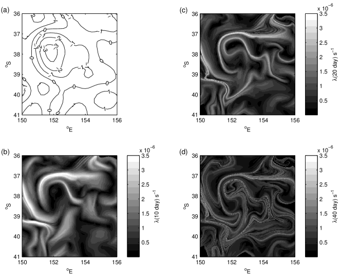
Figure 2: The streamfunction and the finite-time Lyapunov exponents within the study region on 22 November 1997. (a) the streamfunction, $\psi$ ($\times 10^{4}$ m² s^-1) (b) $\lambda(t)$, $t=10$ days (c) $\lambda(t)$, $t=20$ days (d) $\lambda(t)$, $t=40$ days.

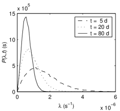
Figure 3: The probability distribution of the finite-time Lyapunov exponents. As expected the distribution narrows with time, but even after 80 days the distribution has not converged.

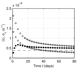
Figure 4: The variation with time of the mean (circles) and standard deviation (squares) of the distribution of finite-time Lyapunov exponents. The open symbols are from the distribution of the maximum Lyapunov exponents, $\lambda$. The solid symbols are from the approximation to the Lyapunov exponents, $\tilde{\lambda}$, calculated from the stretching of randomly aligned initial vectors using Eq. (4). The solid lines show the least-squares fit to the data between 15 and 80 days, using Eqs. (7) and (8). The horizontal dashed line marks the asymptotic value of the Lyapunov exponent, $\lambda_{\infty}$ = 3.84 $\times$ 10^-7 s^-1.

The finite-time Lyapunov exponents are calculated for the study region using the 1997 OI velocity data. A 4th order Runge-Kutta integration with a daily time-step is used to calculate the trajectories of a regular grid of points. The OI velocities are objectively mapped onto a regular grid with a 20 km by 20 km by 5 day spacing, and the data are linearly interpolated in time and space to estimate the velocity along the trajectories. The Jacobian is integrated following Eq. (5) to obtain the matrix ${\bm{M}}^{\text{T}}{\bm{M}}$, and the Lyapunov exponents are then calculated from the eigenvalues $m_{+}$ (Eq. 6). There are two components to the OI velocity field, the mean flow and the velocity anomaly. The optimal interpolation ensures that the anomaly is divergence free, but the mean flow is derived directly from the MCC data and does not have this constraint. While the full velocity field is used to derive the trajectories, only the traceless component of the Jacobian is integrated to obtain $\bm{M}$. As an example of the results, the flow is shown on the 22 November 1997 in Fig. 2, along with the Lyapunov exponents for three different times $t$. In this figure a regular grid of points, with a spacing of 2.2 km, was integrated backwards in time. Trajectories that left the region within which the OI velocities were defined are shown in black. The Jacobian was then integrated forwards along the trajectories to obtain the Lyapunov exponents at a regular grid of points. The streamfunction on November 22 is dominated by an anti-cyclonic eddy with a diameter of approximately 200 km, centred on 38^∘S 152^∘E. The ten day Lyapunov exponents show that the eddy centre is an area of relatively low stretching, with the highest stretching rates being in arms around the eddy. For larger times $t$ the Lyapunov exponent develops a filamentary structure, with the width of the filaments narrowing with time.

The probabability distribution $P(\lambda,t)$ is shown in Fig. 3 for various times $t$. This was calculated from sets of forward trajectories initialised on a 61 $\times$ 51 regular grid. Each set of trajectories began 10 days apart, between 1 January and 12 October 1997. As expected, the distribution of the exponents narrows with time as each trajectory experiences a range of flow conditions. The integration is not continued beyond 80 days as by that time over a third of the trajectories have left the region where the OI velocities are available. The strain of the OI flow in the study region has the mean and standard deviation $\langle\gamma_{+}\rangle=2.5\times 10^{-6}$ s^-1 and $\sigma_{\gamma_{+}}=1.6\times 10^{-6}$ s^-1. The initial stretching is at the rate given by the strain, but the average Lyapunov exponent decreases with time (Fig. 4). The mean Lyapunov exponent is still decreasing at the end of the 80 day integration so the form of $G(\lambda)$ cannot be determined. The Lyapunov exponent $\lambda_{\infty}$ can only be estimated by fitting the relation for the expected time-dependence, Eq. (7) to the data. The least-squares fitted curve to the mean Lyapunov exponent between 15 and 80 days is $\langle\lambda\rangle\sim 0.371/t+4.17\times 10^{-4}/\sqrt{t}+3.84\times 10^{-7}$, where the time, $t$, is in seconds. This gives the estimate $\lambda_{\infty}=4\times 10^{-7}$ s^-1 (or $\lambda_{\infty}=0.035$ day^-1). A similar fit of Eq. (8) to the standard deviation of the Lyapunov exponents gives $\Delta=5\times 10^{-7}$ s^-1. We have not attempted to quantify the uncertainties of these estimates, but, because of the slow convergence, the uncertainties will be relatively large. It could be expected that $P(\lambda,t)$ would become gaussian when $\sigma_{\lambda}<<\lambda_{\infty}$, or when $t>>\Delta/\lambda_{\infty}^{2}$. For the OI flow this will occur when $t>>40$ days, so it is clear that the integration is too short to allow the asymptotic form of $P(\lambda,t)$ to emerge.

The mean value of the Lyapunov exponents approximated from the stretching of an initially randomly aligned vector, $\tilde{\lambda}$, is shown in Fig. 4 for comparison. Because of the random alignment of the initial vector relative to the straining of the flow, the initial stretching is zero. It grows rapidly, and then slowly converges toward the actual value, $\langle\lambda\rangle$. A least squares fit of Eq. (7) to the data between 15 and 80 days gives $\langle\tilde{\lambda}\rangle\sim 0.0428/t+1.59\times 10^{-4}/\sqrt{t}+4.33\times 10^{-7}$. This is consistent with the estimate of $\lambda_{\infty}=4\times 10^{-7}{\text{s}}^{-1}$.

VI Sea-surface temperature

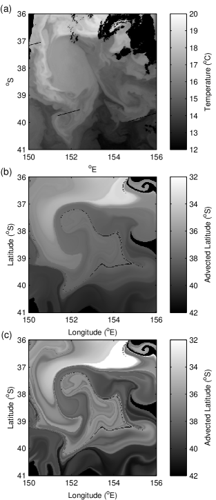
Figure 5: A satellite sea-surface temperature image from 22 November 1997 (a) is compared with SST modelled using the OI velocity field and a first-order equation for a reactive tracer, Eq. (11). The two modelled SST images were generated with the relaxation rates (b) $\alpha=0.05$ day^-1 and (c) $\alpha=0$. In (a) black marks either cloud or invalid data, and in (b) and (c) black marks trajectories which went outside the area in which the OI velocities are defined. The SST image has 1 km pixels, and the modelled data has a 2.2 km resolution.

In this section the formalism developed by Neufeld et al.  Neufeld et al. [2000] and presented in section IV is applied to a satellite image of sea-surface temperature (SST) to test the applicability of the theory in this context. In Fig. 5 an SST image from 22 November 1997 is compared with images produced by the advection of a first-order tracer by the OI flow. The OI streamfunction for this day is shown in Fig. 2, with the dominant feature being an anti-cyclonic eddy. The equation for the tracer (Eq. 11) is integrated along the trajectories, which were calculated backwards from a regular grid with a 2.2 km spacing. The integration is only for 40 days as for longer times too many trajectories leave the area in which the OI velocities are defined. The function $C_{0}$ is taken to be a linear gradient given by the latitude of the trajectory. The tracer field along each trajectory is initialised at its starting latitude. With a relaxation time of $1/\alpha=20$ days (Fig. 5(b)) the broad structures of the modelled SST compare well with what is seen in the satellite image taken on that day (Fig. 5(a)). The anti-cyclonic eddy appears as an area of low gradient, with the northern boundary being marked by a line of strong gradient at 37^∘S. A tongue of warmer northern water comes down the western side of the eddy, and there is a meandering front between latitudes 39^∘S and 40^∘S. Given the extreme simplicity of the sea-surface temperature model the agreement between these images is striking. There are, however, many smaller features which are not resolved in the OI velocity field and so the contours of the modelled SST are smoother than the contours of the actual SST image. If the relaxation rate is set to $\alpha=0$, and the latitude is advected as a conserved tracer, then the same broad patterns are seen (Fig. 5(c)), but the tracer structure becomes more striated than the observed sea-surface temperature. The highest tracer gradients are in the regions of greatest stretching, and the filaments of the $t=40$ day Lyapunov exponents (Fig. 2) are aligned with the contours of the tracer (Fig. 5(c)).

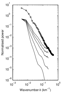
Figure 6: Power spectra of the actual and modelled SST data shown in Fig. 5. The spectra are the mean of the 1-D power spectra taken along 250 km long sections of constant latititude which contain no invalid data. The normalisation is arbitray, having been chosen to aid comparison of the spectra. The spectrum of the actual SST data is shown by the line with circles. The other lines correspond to the modelled SST, with the following values of $\alpha$ (day^-1), from the steepest to the flattest: 0.2, 0.1, 0.05, 0.025 and 0.

The spatial patterns in these images may be quantitatively compared through their power-spectra, Fig. 6. The spectra were taken from the 250 km long constant-latitude sections through the image which only contained valid data. The spectra shown are the averaged cyclic power-spectra, with the sections being detrended and multiplied by a Hann filter before calculating the periodogram. The averaged power-spectra have been given an arbitrary normalisation to allow them to be readily compared. Between inverse wavenumbers of 10 and 100 km the power spectra have a power-law form, with there being a progressive steepening of the spectra as $\alpha$ increases. This has previously been seen in simulations of a first-order tracer in a model flow intended to represent mesoscale turbulence Abraham [1998], and is as expected from theory (Eq. 13). The power-law exponents of the spectra in Fig. 6 are $\beta=2.44\pm 0.04$ (actual SST); $\beta=2.12\pm 0.03$ (conserved tracer); $\beta=2.28\pm 0.03$ ($1/\alpha$ = 40 days); $\beta=2.46\pm 0.04$ ($1/\alpha$ = 20 days); $\beta=2.77\pm 0.09$ ($1/\alpha$ = 10 days); and $\beta=3.47\pm 0.14$ ($1/\alpha$ = 5 days). The spectral exponent of the actual SST data is not significantly different from the exponent of the modelled data with $1/\alpha=20$ days, suggesting that the SST is responding to changes in forcing with a timescale of around 20 days.

The spectrum of the conserved tracer is flatter than the tracer with $1/\alpha=40$ days but, because of the short integration time, the spectrum is still steeper than the $k^{-1}$ form expected for a forced conserved tracer. The 40 day period over which the trajectories are defined is too short to allow a full transfer of variance from low to high wavenumbers. The timescale expected for the transfer between two lengthscales $L_{\max}$ and $L_{\min}$ is $T_{L}=\log(L_{\max}/L_{\min})/\lambda_{\infty}$. For the OI flow $1/\lambda_{\infty}$ = 29 days, so with $L_{\max}/L_{\min}=10$ the timescale for variance transfer through the mesoscale is $T_{L}=70$ days. An integration of at least this length would be needed to allow a spectrum with a slope close to $k^{-1}$ to be established. The 40 day trajectory length is too short to allow the relation between spectral-exponent and the relaxation-rate, given in Eq. (13), to be tested.

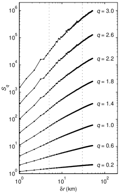
Figure 7: Structure functions, $S_{q}(\delta r)$, calculated using Eq. (14) from the November 22 SST image (Fig. 5(a)). The scaling exponents, $\zeta(q)$, are calculated from a least-squares fit to the structure functions within the range 5 to 30 km, shown by vertical dotted lines. The structure functions are approximately power-law over this range, but roll off toward larger separations, $\delta r$.

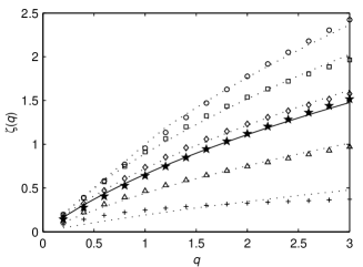
Figure 8: Multifractal scaling exponents of sea-surface temperature. The solid stars ($\star$) are the exponents calculated from the SST data shown in Fig. 5(a). The solid line is a least-squares fit of Eq. (18) to the exponents. The other symbols and the dotted lines mark the scaling exponents calculated from the modelled data and the associated best-fit curve, with the following values of $\alpha$ (day^-1): 0.2 (circle), 0.1 (square), 0.05 (diamond), 0.025 (triangle), 0 (plus).

The multifractal scaling of a tracer may be calculated using the equation for the structure function (Eq. 14). The structure functions of the SST image shown in Fig. 5(a) and of simulated SST were calculated for $\delta r<50$ km, and with $q$ between 0.2 and 3 (Fig. 7). The modelled data were calculated as for Fig. 5(b, c), but with an 80 day integration time and with a range of relaxation rates $\alpha$. The longer trajectory lengths meant that 25% of the trajectories went outside the area where the velocities were defined. Despite the presence of the invalid data, it was still possible to calculate the structure functions as the averaging is only taken over pairs of valid points. The data were detrended before the calculation was made. The resulting scaling exponents, obtained from a least squares regression of $\log(S_{q}(\delta r))$ against $\log(\delta r)$, are shown in Fig. 8. The structure functions of the SST image lie close to the curve derived from the simulated SST with $1/\alpha=20$ days, in agreement with the estimate of $\alpha$ obtained by comparing power-spectra. A least-squares fit of the relation given by Eq. (18) closely follows the SST data, with the best fit dimensionless parameters being $\alpha/\lambda_{\infty}=0.90$ and $\Delta/\lambda_{\infty}=1.12$. With the value estimated for the OI flow of $\lambda_{\infty}=4\times 10^{-7}$ s^-1 this results in $\alpha=0.031$ day^-1, or $1/\alpha=32$ days, and $\Delta=4.5\times 10^{-7}$ s^-1. There is a long chain of assumptions required to allow this estimate to be made, but it doesn’t require an explicit modelling of the flow or, indeed, any knowledge of the flow beyond $\lambda_{\infty}$. Although it is perhaps coincidental, it is pleasing that the value of $\Delta$ is close to that found from an analysis of the finite-time Lyapunov exponents. This suggests that the spatial structure seen in the satellite image is consistent with the representation of SST as an advected first-order tracer. The other dotted lines in Fig. 8 result from fitting the expression for $\zeta(q)$ to estimates made from the simulated SST. The values of $1/\alpha$ (days) predicted from the best-fit curves are 21 (5); 24 (10); 29 (20) and 50 (40), where the actual value is shown in brackets. The curve fitting over-estimates the relaxation time-scale, particularly when the relaxation is rapid. This is likely to be because the derivation of the expression for the fitted curve (Eq. 18) assumes that $P(\lambda,t)$ is gaussian. This is a poor approximation at small times.

Is a 20 day response time for sea-surface temperature reasonable? A one-dimensional turbulence closure model was recently used to simulate seasonal variability of SST in the eastern Tasman Sea, at a similar latitude to the data analysed here, but close to New Zealand Hadfield [2000]. The model used heat and wind forcing derived from meteorological observations. It was found that a perturbation of the atmospheric forcing, applied so that the perturbation was removed at the end of November, had an effect which decayed with a time-scale of one to two months. The response was more complex than a simple first order relation, but nevertheless the response-time inferred from the water column model was of a similar order to that found here. It would be interesting to combine the Lagrangian advection with a water-column model that included realistic heat and wind forcing.

A similar set of assumptions about the dynamics of sea-surface temperature has been used in mesoscale simulations of SST variability by Klein and Hua Klein and Hua [1990]. The focus of these simulations was on the response of SST to episodic bursts of wind. When the mixed-layer is deepened by a wind event the surface temperature is imprinted with a signal from the sub-surface ocean. The mesoscale dynamics below the thermocline may be represented by quasi-geostrophic turbulence. In the ocean interior, temperature is not passive and is dynamically constrained, with a predicted spectral exponent of $\beta=3$ in the sub-mesoscale range. So, when the mixed-layer deepens the sea-surface temperature spectra steepen towards this value. During subsequent stirring of the mixed-layer it was found that temperature variance was transferred towards higher wave-number, resulting in the spectral exponent becoming smaller with time. From this point of view, the processes determing sea-surface temperature spectra are a steepening through episodic wind-mixing and a flattening through horizontal stirring. Following this argument, sea-surface temperature spectra with exponents less than one should be possible during periods of time when the mixed-layer is not deepening for many months, such as over summer. Such flat spectra are not usually observed. An analysis of the spatial pattern in a time-series of SST imagery would allow the relative importance of continuous relaxation and episodic wind-mixing to be resolved.

VII Discussion

Estimates or descriptions of stirring in the surface ocean are rare. In this paper, a spatially and temporally complete velocity dataset was used to calculate the Lyapunov exponents of the flow in a region of the East-Australian current. The mean stirring rate was found to be $\lambda_{\infty}=4\times 10^{-7}$ s^-1, corresponding to a timescale of $1/\lambda_{\infty}=29$ days. The velocity field used is derived using relatively indirect techniques, and only resolves the largest mesoscale features. The question then arises, how reliable is the estimate of the stirring? The observation that tracers advected in ocean flows are filamental suggests that there is a separation between the diffusive length scale and the scale which is controlling the stirring. If, indeed, the larger mesoscale features are dominating the shear then the analysis will be appropriate. This will not be the case in shallow waters, where the eddy length scale is too small to be resolved using the remote methods that are relied on here. There have been beautiful observations made of sub-mesoscale stirring, seen in photographs taken from space of sun-glitter on the sea-surface Munk et al. [2000], Munk and Armi [2001]. These show small eddies, with diameters of only tens of kilometers, organising surface flotsam into filamental slicks. It appears from these photographs that sub-mesoscale eddies may at times dominate the stirring of tracers. In this case, the methods used here would underestimate stirring rates.

From the distribution of the Lyapunov exponents it is clear there is a very wide range in the stretching rates which could be experienced by a patch of tracer in the ocean. Moreover, it would be difficult to predict the stretching of a patch from an Eulerian snapshot of the flow. While the analysis used here is based on a velocity field which could, in principle, be obtained in near real time, predicting the dispersal of either a pollutant or a deliberately released tracer is unlikely to be possible. Small errors in the velocity will lead to a rapid divergence of trajectories. Despite the spread of the probability distribution of Lyapunov exponents it is intriguing to note that the only previous estimate of stirring in the surface ocean, obtained from a satellite image of a deliberately induced phytoplankton bloom Abraham et al. [2000], found a value for the stretching of $\lambda(42\quad\hbox{days})=6\times 10^{-7}$ s^-1. Other estimates of mesoscale stirring from a numerical model ($5.8\times 10^{-7}$ s^-1 Haidvogel and Keffer [1984]) and from a deep tracer release ($3\pm 0.5\times 10^{-7}$ s^-1Ledwell et al. [1993, 1998]) are all of a similar order. The agreement of the values obtained, using very different methods, suggests that the estimate for $\lambda_{\infty}$ found by analysing the OI velocity field is a reasonable one, with the advantage over the tracer-releases that the required data are readily available.

There has been much work recently on the stirring of reactive tracers, particularly phytoplankton, in the surface ocean Franks [1997], Abraham [1998], Bracco et al. [2000], Martin [2000], Scheuring et al. [2000], Károlyi et al. [2000], López et al. [2001], Richards et al. [2001], McLeod et al. [2001]. This research has generally relied on simple models of the ocean flow. The study of Lagrangian chaotic flows, in particular, has allowed the problem to be broken into its simplest components and understanding of the patterns seen in advected tracers has been advanced considerably. The application of this theoretical work has been somewhat hampered by the lack of appropriate oceanic data. The analysis presented here is intended to help alleviate that problem, but is presented as a simple case study only. There are many further directions in which it may be taken. It would be interesting to test the application of the theoretical relationships in a model of ocean turbulence which was not disadvantaged by the short integration times that we were restricted to here. As far as sea-surface temperature is concerned, it would be interesting to carry out a systematic analysis of the whole East-Australian optimally-interpolated dataset. There may be seasonal variations in the estimated value of the response time, $\alpha$, and if these reflect real ocean processes then they will contain information on mixed-layer depth. Since mixed-layer depth is a crucial factor controlling primary production in the ocean, a method for deriving it from remotely sensed data would have great value. As more satellite data becomes available, and as techniques for extracting sea-surface velocities from the temperature data are improved, it is hoped that well resolved surface velocity fields will become widely avaible. Analysis of these will transform our understanding of dispersal processes in the surface ocean.