Stretching of polymers in a turbulent environment

Abstract

The interaction of polymers with small-scale velocity gradients can trigger a coil-stretch transition in the polymers. We analyze this transition within a direct numerical simulation of shear turbulence with an Oldroyd-B model for the polymer. In the coiled state the lengths of polymers are distributed algebraically with an exponent $\alpha=2\gamma-1/De$, where $\gamma$ is a characteristic stretching rate of the flow and $De$ the Deborah number. In the stretched state we demonstrate that the length distribution of the polymers is limited by the feedback to the flow.

1 Introduction

Dilute solutions of long polymers show a fascinating variety of unusal flow phenomena [1, 2]. Recent effects include the formation of vortex pairs in viscoelastic Taylor-Couette flow [3, 4, 5] and a phenomenon called elastic turbulence [6]. While many phenomena in the laminar regime can be understood within simple constitutive equations [1, 2], the interplay with turbulence has remained less clear. In particular, the drag reduction by minute amounts of long polymers in turbulent flows [7] awaits explanation. Various experiments have established that drag reduction comes about when the relaxation time of the polymers is comparable to the fluctuation times in the velocity field [8, 9]. And it is known that a long polymer undergoes a transition to an uncoiled state when exposed to sufficient strain [10, 11]. Our aim here is to study the interaction of a polymer with a turbulently fluctuating flow, in particular the transition from the coiled to the stretched state as the internal relaxation rate becomes comparable to the velocity gradients, and to compare to the theoretical predictions of Balkovsky et al. [12]. Specifically, they predict an algebraic distribution for the trace of the configuration tensor with an exponent that depends linearly on the Deborah number and an internal stretching rate of the flow. Moreover, if the strain is so strong as to uncoil the flow, this process comes to a stop through its effect on small-scale fluctuations of the flow.

2 Model and numerical implementation

We model the polymer by an upper convected Maxwell fluid with a single relaxation time $\lambda$ [13]. The polymer is characterized by the conformation tensor $c_{ij}$. Within a dumb-bell model [1] this tensor can be formed from the end-to-end distance vector $\vec{R}$ as $c_{ij}=\langle R_{i}R_{j}\rangle$ where $\langle\cdots\rangle$ denotes a thermal average. In the coiled state the polymers are spherical and $c$ can be normalized so that $c_{ij}^{\rm eq}=\delta_{ij}$ and $\operatorname{Tr}c=3$. In the Maxwell model the relaxation of the polymers is assumed to be linear, so that the dynamical equations become

$$\frac{D}{Dt}c_{ij}-c_{ik}\partial_{k}v_{j}-c_{jk}\partial_{k}v_{i}=-\frac{c_{ij}-c_{ij}^{\text{eq}}}{\lambda}\,,$$ (1)

with $\lambda$ as the time constant and $D/Dt$ as the convective derivative. The polymers are assumed to be diluted in a Newtonian solvent so that for the flow properties also the Newtonian shear viscosity has to be included. This then defines an Oldroyd-B model [14]. The Oldroyd-B model is able to describe two main features of viscoelasticity, namely normal stress differences and stress relaxation, and has been succesfully applied in the study of vortex pairs in Couette-Taylor flow [5]. The main caveat of this model, the divergence of the conformation tensor when the shear rate of the flow exceeds $1/\lambda$ is usually overcome with the FENE model [1, 15]. However, as predicted by Balkovsky et al. [12] and demonstrated below the extension of the polymer is stabilized through the feedback on the flow once it begins to expand.

We want to study the turbulence of a flow bounded by two surfaces and driven by a volume force that maintains a constant mean shear gradient $S$ (see Fig. 1). This gives an external length scale $L$ (distance between surfaces) and a velocity scale $U$ (twice the velocity difference across the gap). The Reynolds number then is $Re=UL/\nu$ with $\nu$ being the kinematic viscosity, and the Deborah number (characterizing the polymer relaxation) is $De=\lambda U/L$. The dimensionless Navier-Stokes and Oldroyd-B equations become

$$\partial_{t}v_{i}+(v_{k}\partial_{k})v_{i} =-\partial_{i}p+\frac{1}{Re}\partial_{jj}v_{i}+\partial_{j}\tau^{p}_{ij}+f_{i}\,,$$ (2)

$$\partial_{t}c_{ij}+(v_{k}\partial_{k})c_{ij} =c_{ik}\partial_{k}v_{j}+c_{jk}\partial_{k}v_{i}+\frac{c_{ij}-\delta_{ij}}{De}\,.$$ (3)

The relation of stress and conformation tensor is given by

$$\tau^{p}_{ij}=\frac{s}{De\,Re}(c_{ij}-\delta_{ij})\,.$$ (4)

The parameter $s$ in (4) models the strength of the feedback of the polymers on the turbulent flow. Together with the condition of incompressibility,

$$\partial_{i}v_{i}=0\,,$$ (5)

and a prescribed external force $f_{i}$, the set of equations (2) – (4) form a closed system for the variables $v_{i}$, $c_{ij}$ and $p$.

The advantage of writing the Oldroyd-B equation in terms of the conformation tensor $\boldsymbol{c}$ instead of the polymer stress tensor $\boldsymbol{\tau}^{p}$ is that even for $s=0$, when the polymer has no influence on the velocity field and $\tau^{p}_{ij}=0$, it is still possible to monitor $\boldsymbol{c}$ and thus the stretching and rotation of the polymer by the flow.

The model geometry (see Fig. 1) resembles planar Couette flow, i.e. flow between infinite, parallel plates, but with free-slip (or stress-free) boundary conditions along the planes instead of no-slip boundary conditions. With these boundary conditions all fields can be expanded in Fourier series and efficient algorithms can be used. In our dimensionless units the box has dimensions $\Omega=[0,1]\times[0,L_{y}]\times[0,L_{z}]$.

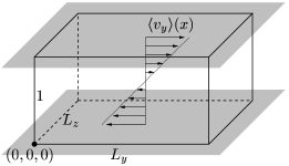
Figure 1: Model geometry: The flow is restricted to the volume between the shaded planes, with no-flux, free-slip boundary conditions at the planes. It is periodically continued in the $y$- and $z$-direction.

While any quantity is taken to be periodic in the $y$- and $z$-direction, boundary conditions in the $x$-direction are somewhat more complicated and must be formulated for each quantity separately. For the velocity, they are

$$\begin{aligned} v_{x}\and{x=0,1}=0\,,&\quad\quad\text{(no flux)}\\ \begin{aligned} \partial_{x}v_{y}\and{x=0,1}&=0\,,\\ \partial_{x}v_{z}\and{x=0,1}&=0\,.\end{aligned}&\quad\quad\text{(no stress)}\end{aligned}$$ (6)

This translates for the solvent stress tensor $\tau^{s}_{ij}$ into

$$\tau^{s}_{ij}\and{x=0,1} =0\quad\text{for }ij=xy,xz,yx,zx,$$ (7)

$$\partial_{x}\tau^{s}_{ij}\and{x=0,1} =0\quad\text{for }ij=xx,yy,zz,yz,zy.$$

The boundary conditions on $\tau^{p}_{ij}$ and $c_{ij}$ must be the same as on $\tau^{s}_{ij}$,

$$c_{ij}\and{x=0,1} =0\quad\text{for }ij=xy,xz,yx,zx,$$ (8)

$$\partial_{x}c_{ij}\and{x=0,1} =0\quad\text{for }ij=xx,yy,zz,yz,zy.$$

Instead of considering the quantities $v_{i}$ and $c_{ij}$ over $\Omega$ and with boundary conditions (6) and (8), one can extend them to $2\Omega:=[-1,1]\times[0,L_{y}]\times[0,L_{y}]$ by reflection at the $x=0$-plane. The equations of motion (2) and (3) are invariant under this transformation. Along the boundary of $2\Omega$, any quantity then obeys periodic boundary conditions and can be expanded in a three-dimensional Fourier series. Mirror symmetry and boundary conditions restrict modes in the $x$-direction to either sines or cosines.

The simulation code is actually written for mixed Fourier ($y,z$) and sine/cosine ($x$) expansion coefficients. The reality condition, relations between coefficients resulting from incompressibility and de-aliasing by the 2/3 rule [16] lead to a further reduction in the number of independent variables. In the end one is left with

$$(4+8\bar{N}_{x})+(5+8\bar{N}_{x})(\bar{N}_{z}+\bar{N}_{y}+\bar{N}_{y}\bar{N}_{z})$$ (9)

independent coefficients, where $\bar{N}_{i}=2N_{i}/3$ for a spatial grid of $(N_{x}+1)\times N_{y}\times N_{z}$ points.

The numerical algorithm employed for time integration is a 5(4)-Dormand-Prince scheme [17] with fixed step size. This scheme uses five evaluations of the right hand side to calculate an approximation for $\boldsymbol{x}(t+\Delta t)$,

$$\boldsymbol{x}(t+\Delta t) =\sum_{i=0}^{5}\alpha_{6i}K_{i}+\mathcal{O}(\Delta t^{6})\,,$$ (10)

$$\text{where}\;\;K_{j} =F(\boldsymbol{x}_{j},t_{j})\,,$$

$$\boldsymbol{x}_{j} =\boldsymbol{x}(t)+\Delta t\sum_{i=0}^{j-1}\alpha_{ji}K_{i}\,,$$

$$t_{j} =t+\gamma_{j}\Delta t\,,$$

with coefficients $\alpha_{ij}$ and $\gamma_{i}$ chosen to minimize the error accumulated over $\Delta t$ [17]. Then, using the derivative $F(\boldsymbol{x}(t+\Delta t),t+\Delta t)\approx F(\boldsymbol{x}_{6},t_{6})$ (which can be kept for the next integration step), a second approximation

$$\boldsymbol{x}^{\prime}(t+\Delta t)=\sum_{i=0}^{6}\alpha^{\prime}_{6i}K_{i}+\mathcal{O}(\Delta t^{5})$$ (11)

of lower order can be obtained. The difference $\delta_{i}=x_{i}-x^{\prime}_{i}$ is used as an estimate for the integration error. In standard applications this error is then used to adapt the step size. However, in a turbulent flow with its ever present fluctuations, variations in this step size are small. So instead we monitor this error estimate by calculating a combination of relative and absolute error,

$$\text{Err}=\max_{i}\frac{|\delta_{i}|}{|x_{i}|+\epsilon}\,.$$ (12)

With $\epsilon=10^{-6}$ an accuracy of $\text{Err}<10^{-5}$ was maintained throughout the integration.

The volume force $f_{i}$ was chosen so as to maintain the mean shear profile (dimensionless form)

$$v^{0}_{y}(x) =\frac{4S}{\pi^{2}}\,\sum_{m=1}^{\text{M}}\frac{\cos\left((2m-1)\pi x\right)}{(2m-1)^{2}}$$ (13)

as an approximation to a linear profile $v^{0}_{y}(x)=S(x-1/2)$. In the simulations, $M=5$, and the Fourier components contained in this mean profile were kept fixed. Thus the force is dynamically adjusted to maintain the prescribed mean shear profile.

One way to initialize the program is to use a random velocity perturbation on the laminar profile and the conformation tensor for the laminar profile. In order to obtain a turbulent state the perturbation has to be about as large as the laminar profile. In turns out, however, that even for moderate Deborah numbers $De\approx 0.1,\ldots,1$ this leads to an extreme overshooting of the conformation tensor and a breakdown of the integration routine.

As a remedy to this we used initial conditions from a turbulent Newtonian flow with equilibrium configuration tensor, $c_{ij}^{\text{eq}}=\delta_{ij}$. The system was then allowed to relax to a statistically stationary turbulent state for a small value of the Deborah number. One of these states was then taken as initial condition for a simulation at a higher $De$. Proceeding in this manner at each change of $De$ the system relaxed to a statistically stationary state within a few time steps and no further numerical integration problems were encountered.

Another numerical problem for Oldroyd-B simulations is connected with the fact that the conformation tensor $c_{ij}$ is by definition positive definite, and that this property is preserved by the Oldroyd-B equations [2] but not in the numerical representation. Through the various Fourier transforms and truncations, this positivity can be lost. If that happens the Oldroyd-B model can develop Hadamard instabilities, and lose its evolutionary character [18]. Thus, if regions with negative $c$ appear, numerical instabilities can arise and the integration can blow up [19]. Fig. 2 shows that such regions indeed do accur, but remain limited to a small fraction of the whole domain, provided $De$ is not too large.

Figure 2: Probability density functions (PDFs) of $\operatorname{Tr}\boldsymbol{c}$ in a turbulent flow at different $De$. There are hardly any regions with negative $\operatorname{Tr}c$ for $De=0.5$ (open triangles) and a significant fraction for $De=0.7$ (open circles). Adding an artifical diffusivity of $\kappa=1/2000$ removes the negative values and leaves the positive distribution essentially unchanged (filled circles). Parameters: $Re=1000$, $S=\partial_{x}\langle v_{y}\rangle=0.5$ and $s=0$. Geometry: $L_{y}=4\pi$, $L_{z}=2\pi$, $N_{x}=32$, $N_{y}=128$, $N_{z}=64$. The PDFs are averaged over 10 snapshots taken at time intervals $\Delta t=5$.

As a partial cure to this problem, Beris et al.[19, 20, 21] introduce an artificial stress diffusion $-\kappa\Delta\boldsymbol{c}$ in the equation of motion for the conformation tensor, where $\kappa$ can be chosen so that it stabilizes the numerics but has negligible influence on the results. Although for the small values of $De$ in Fig. 2 no numerical instability seems to occur, the introduction of a small $\kappa$ does reduce the probability for negative $\operatorname{Tr}\boldsymbol{c}$, while the impact on positive values is much less significant. In the following, calculations for $De\leq 0.5$ are without artificial stress diffusivity ($\kappa=0$). The number of points with $\operatorname{Tr}\boldsymbol{c}<0$ is then negligible. For $De>0.5$, a small $\kappa=1/2000$ is employed to reduce negative tails of PDFs, and for $D=2.0$ it is actually necessary to set $\kappa=1/1000$ to avoid numerical instability. In both cases, a certain probability for negative $\operatorname{Tr}\boldsymbol{c}$ is still unavoidable.

The simulation code is written in Fortran 90 (except the special FFT routines for Cray T90 hardware). It is based on the code used previously [22] for the same model without polymer. Most simulations were done on a Cray T90 vector machine at the John von Neumann Institute for Computing at the Research Centre Jülich. A typical run with a resolution of $N_{x}=32$, $N_{y}=128$, $N_{z}=64$ over $50$ time units costs roughly $26500$ CPU seconds and needs 62 megawords of memory.

3 Statistics of polymer elongation

Balkovsky et al. [12] discuss the behaviour of the PDF for the polymer extension $R=(\operatorname{Tr}\boldsymbol{c})^{1/2}$. For a passive polymer, they predict a power law decay of the tails ($R\rightarrow\infty$), as long as the (dimensionless) relaxation time of the polymer $De$ is smaller than the inverse shear rate $1/(2\gamma)$ of the underlying turbulent flow,

$$\mathcal{P}(R)\sim R^{-\alpha-1}\,.$$ (14)

The exponent $\alpha$ depends on $De$ and $\gamma$. For relaxation times near the inverse Lyapunov exponent, $\alpha$ is given in linear approximation by

$$\alpha\sim\frac{1}{De}-2\gamma\,.$$ (15)

For Deborah numbers smaller than $De_{cr}=1/(2\gamma)$ the exponent $\alpha$ is positive and (14) actually describes an algebraic decay. This corresponds to the majority of the polymer molecules being near their equilibrium elongation. However, for values above the critical Deborah number $De_{cr}=1/(2\gamma)$ the exponent $\alpha$ becomes negative and the probability density function for $R$ is no longer normalizable. At this point the assumption of a passive polymer becomes unphysical. Balkovsky et al. [12] then argue that the feedback from the polymer to the flow field limits the extension, such that $\mathcal{P}(R)$ decays again for large $R$. The majority of the molecules is then stretched to some finite value of $R$, at which $\mathcal{P}(R)$ is maximal. The contribution of the polymer stress $\tau^{p}$ to the right hand side of the Navier-Stokes equation should then be of the same order of magnitude as the advective term $\vec{v}\cdot\nabla\vec{v}$.

The quantity directly accessible from the simulations is $\operatorname{Tr}\boldsymbol{c}=R^{2}$. The PDFs for $R^{2}$ and $R$ are related through

$$\mathcal{P}(R)\,dR=\mathcal{P}(R^{2})\,dR^{2}=2R\,\mathcal{P}(R^{2})\,dR\,.$$ (16)

A power law distribution for one quantity implies one for the other, and the exponents are related by

$$\mathcal{P}(\operatorname{Tr}\boldsymbol{c})\sim\left(\operatorname{Tr}\boldsymbol{c}\right)^{-\beta}\Leftrightarrow\mathcal{P}(R)\sim R^{-\alpha-1}\,,$$ (17)

with $\alpha=2(\beta-1)$.

Figure 3: PDFs of $\operatorname{Tr}\boldsymbol{c}$ in turbulent flow for different values of $De$. The straight lines in the lower frame follow from algebraic fits over the ranges over which they are shown. Every data point corresponds to one bin. Parameters: $Re=1000$, $\partial_{x}\langle v_{y}\rangle=0.5$ and $s=0$. $\kappa=1/2000$ for $De\geq 0.6$. Geometry: $L_{y}=4\pi$, $L_{z}=2\pi$, $N_{x}=32$, $N_{y}=128$, $N_{z}=64$. The initial condition was the same for all $De$. The PDFs are averaged over 10 snapshots taken at time intervals $\Delta t=5$.

Fig. 3 demonstrates these power tails in PDFs obtained from turbulent simulations for different $De$. The exponents $\beta$ are obtained from the slope in a log-log plot (lower graph). The region where the power law actually holds starts when $\mathcal{P(\operatorname{Tr}\boldsymbol{c}})$ drops below about $10^{-1}$ and extends right up to the statistical accuracy limit for larger $\operatorname{Tr}\boldsymbol{c}$.

Figure 4: Exponents extracted from Fig. 3 ($De\leq 0.8$, squares) and the equivalent for ($De=2.0$, $s=0.01$, open circle). The regression line derived from the solid squares intersects with $\alpha=0$ for $1/De=0.61=2\gamma$. Note that the open circle for the situation of uncoiled polymers also lies on the line.

From the exponents determined in Fig. 3, the Lyapunov exponent $\gamma$ (and with it, the critical Deborah number) can be obtained by plotting $\alpha$ as a function of $1/De$, as in Fig. 4, and extrapolating the linear relationship to $\alpha=0$. Note that the three points corresponding to $De=0.6$, $0.7$ and $0.8$ fit the line surprisingly well. The deviation for $De=0.5$ could be attributed to the fact that only this simulation is done with $\kappa=0$. Also, $De=0.5$ is farthest from the (extrapolated) critical Deborah number.

Figure 5: Time evolution of $\langle\operatorname{Tr}\boldsymbol{c}\rangle$ for $De>De_{cr}$. Without feedback through the flow the polymer length diverges. With feedback ($s\neq 0)$ it stabilizes. The horizontal dotted lines mark the time average of the solid points; these averages decrease with increasing coupling strength $s$.

From the data on the exponents one can extract that for $De$ larger than $1/0.61$ the polymer distribution without feedback is no longer normalizable, the polymers go into a stretched state. This stretching is terminated by their feedback on the flow, as we will now demonstrate. To this end we analyze the time evolution of $\langle\operatorname{Tr}\boldsymbol{c}\rangle$ in Fig. 5. The trace starts at the equilibrium value $\operatorname{Tr}\boldsymbol{c}=3$ at $t=0$. For $De<De_{cr}$ it increases and then stabilizes at a finite value, indicating a certain stretching of the polymer. For $De>De_{cr}$ it increases monotonically, if there is no feedback to the flow ($s=0$), but stabilizes at finite values for $s\neq 0$. The larger the feedback, the smaller the mean values.

In an additional calculation for $De=2.0$ and $s=0$ (see Fig. 5), $\langle\operatorname{Tr}\boldsymbol{c}\rangle$ grows more or less exponentially, as expected, with a rate $d\ln\langle\operatorname{Tr}\boldsymbol{c}\rangle/dt\approx 0.18$. The difference between $1/De_{cr}=0.61$ and $1/De=0.5$ gives a growth rate of about $0.1$. The difference is perhaps connected to the use of different averages in the calculation of the exponents.

4 Conclusions

The full numerical simulations for an Oldroyd-B constitutive equation in a turbulent shear flow support the calculations of Balkovsky et al. and demonstrate and algebraic distribution of polymer lengths below the coil-stretch transition. Above the transition the calculations also show that the potentially infinite stretching of the polymers is limited by their modulation of the small-scale flow properties.

References

- [1] R. B. Bird, R. C. Armstrong, O. Hassager, Dynamics of polymeric liquids, volume 1 (Fluid mechanics), volume 2 (Kinetic theory), John Wiley & Sons, 1987.
- [2] D. D. Joseph, Fluid dynamics of non-Newtonian liquids, Springer, New York, 1990
- [3] A. Groisman, V. Steinberg, Phys. Rev. Lett. 78 (1997) 1460.
- [4] K. A. Kumar, M. D. Graham, Phys. Rev. Lett. 85 (2000) 4056.
- [5] M. Lange, B. Eckhardt, Phys. Rev. E 64 (2001) 027301.
- [6] A. Groisman, V. Steinberg, Nature 405 (2000) 53.
- [7] B. A. Toms, In Proc. Int. Cong. on Rheology, volume 2, pp. 135–141, North-Holland, Amsterdam, 1949.
- [8] J. L. Lumley, Ann. Rev. Fluid Mech. 1 (1969) 367–384.
- [9] N.S. Berman, Ann. Rev. Fluid Mech. 10 (1978) 47–64.
- [10] S. Chu, Rev. Mod. Phys. 70 (1998) 685.
- [11] R. Rzehak, W. Kromen, T. Kawakatsu, W. Zimmermann, Eur. Phys. J. E 2 (2000) 3.
- [12] E. Balkovsky, A. Fouxon, V. Lebedev, Phys. Rev. Lett. 84 (2000) 4765–4768.
- [13] J. C. Maxwell, Phil. Trans. Roy. Soc. A157 (1867) 49–88.
- [14] J. G. Oldroyd, Proc. Roy. Soc. A200 (1950) 523–541.
- [15] R.G. Larson, E.S.G. Shaqfeh, S.J. Muller, J. Fluid Mech. 218 (1990) 573.
- [16] C. Canuto, M. Y. Hussaini, A. Quarteroni, T. A. Zang, Spectral methods in fluid dynamics, Springer, New York, 1988.
- [17] E. Hairer, S. P. Nørsett, G. Wanner, Solving ordinary differential equations I – nonstiff problems, Springer, Berlin, 1993.
- [18] F. Dupret, J. M. Marchal, J. Non-Newtonian Fluid Mech. 20 (1986) 143–171.
- [19] A. N. Beris, C. D. Dimitropoulos, Comput. Methods Appl. Mech. Engng. 180 (1999) 365–392.
- [20] R. Sureshkumar, A. N. Beris, J. Non-Newtonian Fluid Mech. 60 (1995) 53–80.
- [21] A. N. Beris, R. Sureshkumar, Chem. Engng. Science 51 (1996) 1451–1471.
- [22] J. Schumacher, B. Eckhardt, Europhys. Lett. 52 (2000) 627–632.