Modeling Vocal Fold Motion with a New Hydrodynamic Semi-Continuum Model

Abstract

Vocal fold (VF) motion is a fundamental process in voice production, and is also a challenging problem for direct numerical computation because the VF dynamics depend on nonlinear coupling of air flow with the response of elastic channels (VF), which undergo opening and closing, and induce internal flow separation. A traditional modeling approach makes use of steady flow approximation or Bernoulli’s law which is known to be invalid during VF opening. We present a new hydrodynamic semi-continuum system for VF motion. The airflow is modeled by a quasi-one dimensional continuum aerodynamic system, and the VF by a classical lumped two mass system. The reduced flow system contains the Bernoulli’s law as a special case, and is derivable from the two dimensional compressible Navier-Stokes equations. Since we do not make steady flow approximation, we are able to capture transients and rapid changes of solutions, e.g. the double pressure peaks at opening and closing stages of VF motion consistent with experimental data. We demonstrate numerically that our system is robust, and models in-vivo VF oscillation more physically. It is also much simpler than a full two-dimensional Navier-Stokes system.

PACS numbers: 43.70Bk, 43.28Ra, 43.28Py, 43.40Ga.

1 INTRODUCTION

Vocal folds (VF) are the source of the human voice, and their motion is a fundamental process in speech production. In recent years, mathematical modeling of vocal folds has been pursued as a viable alternative to direct experimental studies using strobovideolaryngoscopy or electroglottography techniques. Numerical simulations of VF models then provide us with a valuable tool to understand, monitor and predict various behaviors of normal and disordered voices in vivo. Together with models of vocal tract, one can construct a voice simulator which clinicians, speech therapists, voice teachers, and otolaryngologists can use to help with their skill improvement, diagnosis and patient treatment.

Since VF motion is mechanical and results from the nonlinear interaction of airflow and elastic response of VF, partial differential equations (PDEs) can be written down from classical continuum mechanics based on our knowledge of VF structures and air flow characteristics. However, the complexity involved is daunting, both in terms of airflow and VF structure, for a direct simulation of a complete set of governing equations. Also it is not necessary that one needs all the details of such a solution to describe the main VF properties. Modeling effort is required to build a smaller set of equations that can capture the essential features of VF dynamics. In the past decade, much progress has been made in modeling the elastic aspect of VF. There are by now a hierarchy of elastic models for VF, from the two mass model of Ishizaka and Flanagan [1], Bogaert [2], to 16 mass as well as the continuum model of Titze and coworkers [3, 5, 6, 7]. However, the modeling of airflow or the fluid aspect of VF is much less explored.

There are broadly two types of approaches in treating the glottal flow. One approach is to combine the Bernoulli’s law in the bulk of the flow (steady flow approximation) with empirical formulas in boundary layer, flow separation and wake [1, 2, 3, 8]. This approach oversimplifies the flow in the sense that PDEs are approximated by algebraic equations. Though the approach is a working method for building simple models, it clearly introduces drastic approximations. For example, it was realized [9] and concluded [10] that Bernoulli’s law is not valid during one-fifth of the VF vibration cycle, especially at VF opening and closure. This lack of accuracy as a result of deviating significantly from the original PDEs is a major drawback of the empirical approach. The other approach is to directly simulate the two dimensional Navier-Stokes (NS) system. Two dimensionality is a common assumption for vocal flows [8]. Alipour et al. formulated a steady state simulation with a given glottal geometry [11]. Both [8, 11] appeared to have been done for fixed channel shape, or in other words, in-vitro VF. To accurately model the pulsating nature of the flow during VF vibration however, a time dependent solution is more appropriate. Yet in such a case, it is highly difficult to resolve the flows in the presence of moving boundaries, closures, and flow separation. Existing works are few in this direction although a lot of measurements on the flow characteristics such as intraglottal air pressure and flow velocity have been made, by Titze and others [8, 10, 16, 12, 13, 14, 15, 11, 17].

The current status of flow modeling calls for a systematic study of reduced PDE flow models and their coupling with existing elastic models. In this paper, we develop an intermediate in-vivo PDE model system so that original airflow PDEs are approximated by reduced PDEs, not algebraic equations. Consider for now that the two sides of VF are symmetric to each other across the centerline, the methodology could be extended to the asymmetric case. The air flow is modeled by a quasi-one dimensional (vertical or upward direction) system of flow equations. The flow variables (pressure, velocity, density) are averaged quantities over the channel cross section of the corresponding ones in two dimensional NS system. Assuming that the flow is predominantly in the vertical direction, which is reasonable before flows become turbulent in the exit region, we derive the model flow system from the two dimensional isentropic compressible Navier-Stokes equations, see the appendix, also [18]. If the channel is not changing in time, the system reduces to the familiar quasi-one dimensional gas dynamic equations in studying duct flows in aerodynamics [19, 20, 21, 22]. If the channel varies in time, there is an additional source term in the flow momentum equation, which turns out to be essential for drawing connection with the Titze theory of small VF oscillation [23]. One can regard the reduced airflow system as a coarse-grained NS system which contains the Bernoulli’s law as a special case, and inherits time dependent convection mechanisms from the full two dimensional NS system. The advantage is that the system is able to handle time dependent effects, such as rapid pressure and velocity changes, during VF opening and closing; moreover, it is a lot simpler to simulate numerically because all the unknown dependent variables are one dimensional in space. Such a system will be coupled to an improved two mass model [2] for the VF cross section area to form a complete VF model. The VF cross section area appear as variable coefficients in the quasi-one dimensional air flow system. The VF motion is described by how VF cross section area varies in time.

The rest of the paper is organized as follows. In section 2, we introduce the equations of the model, and address related modeling issues. In section 3, we discuss numerical method and numerical results of model simulation. We show numerically that our model is able to generate VF motion in-vivo, and recover several known VF characteristics supported by experimental measurements, for example, unequal double pressure peaks at VF opening and closure. We also show the robustness of our model by varying subglottal pressure and plotting how air volume velocity (air flux) changes as a function of time. Our results reach complete qualitative agreement with existing VF flow data. The conclusion is in section 4, and acknowledgement in section 5. Section 6 is the appendix on the derivation of our reduced flow model from the two dimensional compressible Navier-Stokes system. Table 1, figure captions and figures follow the references.

2 THE SEMI-CONTINUUM MODEL

Suppose the larynx is a two dimensional channel with a finite mass elastic wall of cross section width $A(x,t)$, and length $2L$. The vocal fold is lumped into a sum of two masses connected by a spring, and each mass is connected to solid wall by a spring and a damper, the classical scenario in the two mass model [1, 2]. The air flows from $x=-L$ to $x=L$, and is modeled by the quasi-one dimensional system derived in [18]:

$\bullet$ conservation of mass:

$$(A\rho)_{t}+(\rho\,u\,A)_{x}=0,$$ (2.1)

$\rho$ air density, $u$ air velocity;

$\bullet$ reduced momentum equation:

$$(\rho uA)_{t}+(\rho u^{2}A)_{x}=-(pA)_{x}+A_{x}p+{\rho uA_{t}},$$ (2.2)

$p$ air pressure.

Assuming that the temperature is maintained as constant, so the airflow is isothermal, then the equation of state is:

$$p=a^{2}\rho,$$ (2.3)

where $a$ is the speed of sound. The cross section width $A$ is a piecewise linear function in $x$ determined by the locations of the two masses ($y_{1}$, $y_{2}$), in the classical two-mass model system (Bogaert [2], Ishizaka and Flanagan [1]):

$$m_{1}y_{1}^{\prime\prime} + r_{1}y_{1}^{\prime}+k_{1}(y_{1}-y_{0,1})+k_{12}(y_{1}-y_{2}+y_{0,12})=F_{1},$$ (2.4)

$$m_{2}y_{2}^{\prime\prime} + r_{2}y_{2}^{\prime}+k_{2}(y_{2}-y_{0,2})+k_{12}(y_{2}-y_{1}-y_{0,12})=0,$$ (2.5)

where $F_{1}=L_{g}\int_{-L}^{x_{s}}\,p\,dx$, $L_{g}$ the transverse (to the flow) dimension of vocal fold; $y_{i}$’s are VF openings at locations $x_{i}$’s, $-L<x_{1}<L=x_{2}$; $x_{s}=x_{2}$ if there is no flow separation, and $x_{s}=$ the location of flow separation if it occurs. The $m_{i}$, $r_{i}$, $k_{i}$, $i=1,2$, are mass density, damping and elastic spring constants. Mass one (lower mass) is situated near the VF entrance, and mass two (upper mass) is located towards the exit of the glottal region. Following Bogaert[2], $x_{s}$ will be estimated by an empirical formula on the degree of divergence of the VF. Our complete VF model is the coupled system (2.1)-(2.5).

To make the paper self-contained, the derivation of (2.1)-(2.2) is included in the appendix. The flow variables in the quasi-one dimensional system are averages over the channel cross section of the corresponding ones in two-dimensional flows. The viscous effect in the flow produces the term $\rho uA_{t}$ from the no-slip boundary condition of the two-dimensional flows. Without this term, the above system is a familiar one used in gas dynamics (see [21, 19, 20, 22] and references therein) for modeling flows through ducts with variable cross section. It is shown [18] that this extra term is critical in transferring energy from airflow into the VF, as the Titze theory [23] predicted. We have ignored the viscous terms in the momentum equation for simplicity, they appear to be higher order.

Two mass model (2.4)-(2.5) is a recent improvement [2] of the original IF72 [1] in that flow separation point is not always at the VF exit, instead it depends on the glottal geometry. Flow separation basically refers to a change of flow behavior from being attached to the VF cover via a viscous boundary layer to a developed free jet with vortical structures and turbulent wake. Because of the vortical buildup, pressure near the wall is typically low, and can be approximated by setting it to zero (or ambient pressure) as done on mass two in (2.5) when there is no vocal tract. In converging glottis, there is no flow separation, however in diverging glottis, it occurs if the diverging angle is large enough. It is as yet a challenging problem (no simple theoretical prediction) to decide for a flow when and where separation occurs. It is expedient for modeling purpose to adopt a working hypothesis supported by experiments [2, 8]:

$$y_{2}/y_{1}<1.1\Longrightarrow\;\;x_{s}=x_{2},$$ (2.6)

$$y_{2}/y_{1}>1.1\Longrightarrow\;\;x_{s}=x_{1}+{(x_{2}-x_{1})y_{1}\over 10(y_{2}-y_{1})},\;y_{s}=1.1y_{1}.$$ (2.7)

Notice that the flow separation location is a variable depending on the diverging angle. It is worth pointing out that the assumptions we made for deriving the reduced flow model are all valid prior to the separation point. We expect to see a deviation after the flow separation point between the reduced flow model and the fully two dimensional NS solutions; however, flow pressure post separation is not used in (2.5). Thus our reduced flow model matches perfectly with the improved two-mass model [2].

We also adopt the elastic collision (stopping) criterion in [1, 2] when the two sides of VF approach each other and close. When $y_{i}$’s are smaller than a critical level $y_{c}$, then VF is considered closed. Following [1, 2], $(m_{i},r_{i},k_{i})$ ($i=1,2$) are adjusted to closure values. In this case, the flow equations are solved only over $x\in[-L,x_{1}]$, and in (2.4)-(2.5) the pressure force is adjusted to $F_{1}=L_{g}\int_{-L}^{x_{1}}p\,dx$. Due to constant input pressure $p_{0}$, pressure at $x_{1}$ builds up. The two mass ODE’s (ordinary differential equations) are still running even during VF closure, and in due time the increased pressure reopens VF.

The VF model system is posed as an initial boundary value problem on $x\in[-L,L]$, with inlet boundary condition $(\rho,u)(-L,t)=(\rho_{0},u_{0})$, and a zero Neumann type boundary condition at exit $(\rho_{x},u_{x})(L,t)=0$. The advantage of such Neumann type boundary conditions is that it helps the flow to go out of the computational domain, which is needed for a stable numerical method free of numerical boundary artifacts. Our numerical experiments suggest that the above treatment works fine.

The major difference between our model and that of Bogaert [2] is that we do not make quasi-steady approximation on the flow variables, instead we integrate time dependent system (2.1)-(2.2). This turns out to be particularly important for capturing transients near closure and reopening stages of VF motion.

It is helpful to put the system (2.1)-(2.2) into a rescaled form. Let $v=u/a$, $a$ the speed of sound. Then:

$${1\over a}(Ap)_{t} + (pvA)_{x}=0,$$

$${1\over a}(pvA)_{t} + (pv^{2}A)_{x}=-(pA)_{x}+A_{x}p+pvA_{t}/a,$$ (2.8)

where typically $v=u/a\approx 0.1$, the Mach number. If we use the convenient cm-g-ms unit, $a=35\,cm/ms$, $1/a$ is a small parameter. If we ignore the terms with $a$, we have exactly Bernoulli’s law for steady flows. However, these seemingly small terms are essential especially during opening stage of VF, and should be kept for an accurate time-dependent solution.

3 NUMERICAL METHOD AND SIMULATION RESULTS

For given VF shape, $A(x,t)$, the flow system (2.1)-(2.2) is of the form:

$$U_{t}+(F(U))_{x}=G(U),$$ (3.1)

so called conservation law (see [24] and references therein) with lower order source term $G$. The function $F$ is the flux function. We implemented a first order finite difference method, where time marching is split into two steps. In the first step ($t=nk\rightarrow(n+{1\over 2})k$), we solve the conservation law $U_{t}+(F(U))_{x}=0$ with explicit Lax-Friedrichs method [24]:

$$U_{j}^{n+{1\over 2}}={1\over 2}(U_{j-1}^{n}+U_{j+1}^{n})-{k\over 2h}\left(F(U_{j+1}^{n})-F(U_{j-1}^{n})\right),$$ (3.2)

where $k$ and $h$ are time step and spatial grid size. Here $k$ must be small enough to ensure stability of the difference scheme and to keep the computed flow velocity positive (no back flow is allowed). In step two ($t+{k\over 2}\rightarrow t+k$), we update the solution from $U^{n+{1\over 2}}$ to $U^{n+1}$ by implicitly integrating ODEs: $U_{t}=G(U)$ in flow equations, and the two mass equations (2.4)-(2.5); where we apply central differencing in space and backward differencing in time. In the first step, $U$ is updated using VF shape $A$ at time $t=nk$; in the second step, the ODEs from two mass system and source terms are solved to update solutions to $(n+1)k$. We point out that when VF approach closure, the ODE’s in step two become rather stiff, and this is the main reason to use implicit backward differencing in time [25]. The time step $k$ is a variable. It is smaller when VFs are closing and the equations are stiff, and is larger when VFs are opening up.

The parameters used in our calculation are: space grid size $h=0.01125$, variable time step $k\in(10^{-6},10^{-4})$. The time unit is ms, length unit cm, $2L=0.225\,cm$, speed of sound $a=35\,cm/ms$, $u_{0}=4\,cm/ms$, $p_{0}=7840$ $dynes$ $cm^{-2}$. Other two mass model parameters are in Table 1. In runs not shown, we have reduced $h$ to half or even smaller sizes, and observed similar findings as reported below.

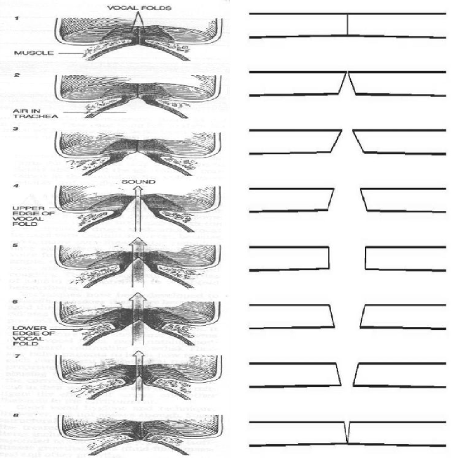
Figure 1: VF Vibration: left column — p. 113 of Sataloff [26], right column — simulated VF with our model (2.1)-(2.5).

Now we describe our numerical results, and compare with figures in the literature or those from experimental measurements. In Figure 1, we show a comparison of a cycle of VF vibration. The left column is the figure on page 113 of Sataloff’s Scientific American article [26], the right column is a plot of our numerically simulated VF vibration cycle. The resemblance is clear. A web animation is also available [27].

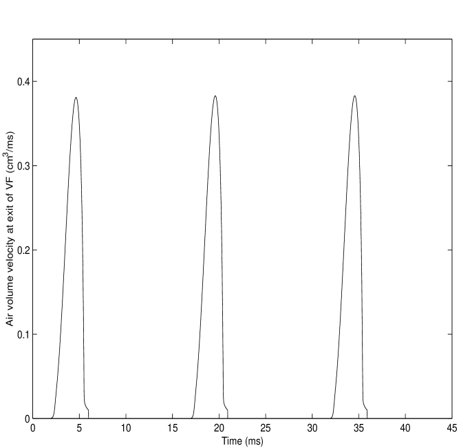
Figure 2: Simulated VF volume velocity (air flux, $cm^{3}/ms$ ) vs time at exit of VF from model (2.1)-(2.5).

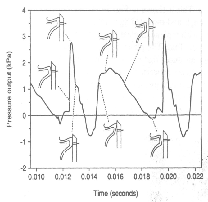
Figure 3: Experimentally measured intraglottal pressure on excised canine larynx, see Fig. 8 on page 426 of Titze [12].

In Figure 2, we show our computed air volume velocity (air flux) at the exit of VF, which compares well with Fig 6, Fig 7, Fig 8 of Story and Titze [3]. Notice that the airflux goes down to zero gradually at VF closing then drops down abruptly to zero. The drop is due to the cutoff introduced in the two mass model for closure, the $y_{c}$. Below $y_{c}$, the cross section area $A$ becomes very small, and the flow calculation becomes rather stiff. In other runs (not shown), we have observed that increasing $y_{c}$ will shorten the curved portion and straighten up the plot near closures ($t\approx 6,21,36$ ms). The air volume velocity shows asymmetry, steeper on the right side than on the left side, consistent with Fig. 3b of Titze [23].

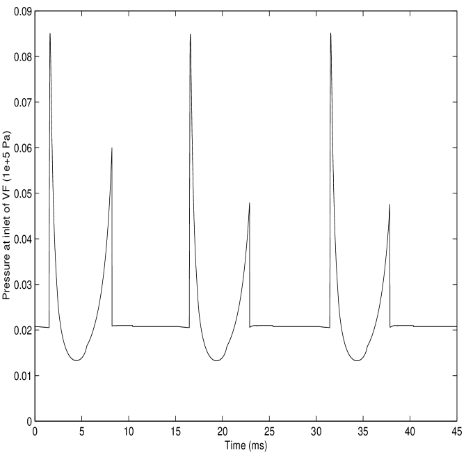
Figure 4: Computed pressure ($10^{5}$ Pa) change in time at the point right before lower mass.

Figure 3 is the experimentally measured intraglottal pressure on an excised canine larynx from [12] (Fig. 8 there) and [13], which showed the double peak (intraglottal) pressure structure respectively at VF opening and closing. Figure 4 is our computed pressure at the grid point before lower mass. The double peaks are present and resemble well those in Figure 3, only that ours are steeper and higher. Several factors contribute to the difference: (1) we used inviscid flow model while there was physical air viscosity in experiments that smooth the solutions, (2) the closure treatment of two mass model differs from the actual VF closure, (3) Figure 3 plots the pointwise pressure, not an average pressure over glottis. At the qualitative level however, our model solutions are in full agreement with the experimental finding. Notice that the second peak is lower than the first.

To the best of our knowledge, the experimentally observed unequal double pressure peaks [12, 13], have not been computed previously in a VF model without coupling to vocal tract. The experiment had no vocal tract load. In Story and Titze [3], a computed two peak intraglottal pressure plot was given (see Fig 11 [3]) using their three mass VF model; however, there is additional coupling to vocal tract or an additional subglottal system. Also their computed second peak appeared higher than the first peak. The fact that our model can recover the experimental double pressure peaks renders strong support for its validity and value.

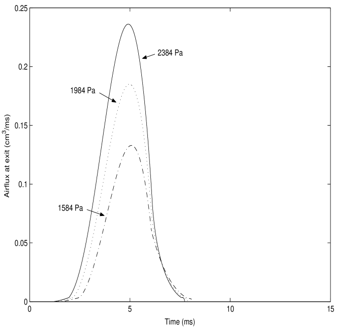
Figure 5: The computed air volume velocity for three values of subglottal pressures.

We also tested our model robustness under pressure variation. In Figure 5, we show a plot of air volume velocity vs time at VF exit for three subglottal pressures: 1584 Pa, 1984 Pa, 2384 Pa with other parameters same as in Table 1. We see that as subglottal pressures increase with other parameters fixed, air volume velocity curves get higher (at peaks) and steeper (at two sides). This agrees very well with Fig. 2.14(a), page 78, of K. Stevens [17], and is another strong support for our model.

In Figure 6, we show an air particle velocity at VF exit (after upper mass) over three vibration cycles for subglottal pressure 2384 Pa, which agrees qualitatively with Fig 3c, page 1538, of Titze [23]. For Figure 6, a small amount of additional numerical diffusion is added in (2.1)-(2.2).

4 CONCLUDING REMARKS

In this paper, we introduced a new semi-continuum VF model consisting of a reduced PDE flow system [18] and a recent two mass elastic system [2]. The flow part of the model is more physical than a traditional treatment with Bernoulli’s law yet much simpler than a full two dimensional Navier-Stokes system. The reduced PDEs are derivable from the two dimensional compressible Navier-Stokes system, and are much more economical for computation. We demonstrated numerically that the model solutions are in qualitative agreement with known VF experimental measurements. In future work, we plan to couple the flow model with more physiological elastic VF models, such as [3]; compute with higher order finite difference methods [24] for attaining more accuracy; analyze qualitative properties (phonation thresholds) of model solutions using bifurcation methods; and incorporate additional viscous effects in the flow.

5 ACKNOWLEDGEMENTS

The authors wish to thank Profs. I. Titze and F. Alipour for helpful conversations and email communication on VF modeling, and for their recent work [7]. The authors would like to thank Dr. J. M. Hyman for suggesting references [22, 26].

6 APPENDIX: DERIVATION OF REDUCED FLOW SYSTEM

We derive the fluid part of the model system assuming that the fold varies in space and time as $A=A(x,t)$. Consider a two dimensional slightly viscous subsonic air flow in a channel with spatially temporally varying cross section in two space dimensions, $\Omega_{0}=\Omega_{0}(t)=\{(x,y):x\in[-L,L],y\in[-A(x,t)/2,A(x,t)/2]\}$, where $A(x,t)$ denotes the channel width with a slight abuse of notation, or cross sectional area since the third dimension is uniform. The two dimensional Navier-Stokes equations in differential form are (Batchelor [28], page 147):

$\bullet$ conservation of mass:

$$\rho_{t}+\nabla\cdot(\rho\,\vec{u})=0;$$ (6.1)

$\bullet$ conservation of momentum:

$$(\rho\vec{u})_{t}=-\nabla\cdot(\rho\,(\vec{u}\otimes\vec{u}))+div(\sigma\cdot\vec{n}\,);$$ (6.2)

where $\sigma$ is the stress tensor, $\sigma=(\sigma_{ij})=-p\mbox{$\delta$}_{ij}+d_{ij}$, and:

$$d_{ij}=2\mu\,(e_{ij}-{\frac{div\vec{u}}{3}}\mbox{$\delta$}_{ij}),\;\;e_{ij}={\frac{1}{2}}(u_{i,x_{j}}+u_{j,x_{i}}),\;\;(x_{1},x_{2})\equiv(x,y);$$

$\mu$ is the fluid viscosity; $\Omega(t)$ is any volume element of the form: ($\vec{u}=(u_{1},u_{2})$)

$$\Omega(t)=\{(x,y):x\in[a,b]\subset[-L,L],y\in[-A(x,t)/2,A(x,t)/2].\}.$$ (6.3)

The equation of state is either polytropic or isothermal.

The boundary conditions on $(\rho,\vec{u})$ are:

(1) on the upper and lower boundaries $y=\pm A(x,t)/2$, $\rho_{y}=0$, and $\vec{u}=(0,\pm A_{t}/2)$, the velocity no slip boundary condition;

(2) at the inlet, $x=-L$, $p=p_{0}$, given subglottal pressure, $(u_{1},u_{2})=(u_{1,0},u_{2,0})$, given input flow velocity. At the exit. $(p,u_{1},u_{2})_{x}=0$, to help the waves go out of the domain freely.

We are only concerned with flows that are symmetric in the vertical. For positive but small viscosity, the flows are laminar in the interior of $\Omega_{0}$ and form viscous boundary layers near the upper and lower edges. The vertically averaged flow quantities are expected to be much less influenced by the boundary layer behavior as long as $A(x,t)$ is much larger than $O(\mu^{1/2})$. We also ignore effects of possible flow seperation inside $\Omega_{0}$ when it becomes divergent with large enough opening.

Let us assume that the flow variables obey:

$$|u_{1,y}|\ll|u_{1,x}|,\;|u_{2,y}|\ll|u_{1,x}|,\;{\rm away\;from\;boundaries\;of\;}\Omega_{0},$$

$$|\vec{u}_{y}|\gg|\vec{u}_{x}|,\;{\rm near\;the\;boundaries\;of\;}\Omega_{0},$$

$$|\rho_{y}|\ll|\rho_{x}|,\;{\rm throughout\;}\Omega_{0}.$$ (6.4)

These are consistent with physical observations in the viscous boundary layers (Batchelor [28], page 302), namely, there are large vertical velocity gradients, yet small pressure or density gradients in the boundary layers. The boundary layers are of width $O(\mu^{1/2})$. Denote by $\overline{\rho}$, $\overline{u}_{1}$, the vertical averages of $\rho$ and $u_{1}$. Note that the exterior normal $\vec{n}=(-A_{x}/2,1)/(1+A_{x}^{2}/4)^{1/2}$ if $y=A/2$, $\vec{n}=(-A_{x}/2,-1)/(1+A_{x}^{2}/4)^{1/2}$ if $y=-A/2$.

Let $a=x$, $b=x+\mbox{$\delta$}x$, $\mbox{$\delta$}x\ll 1$, $t$ slightly larger than $t_{0}$. We have:

$${\frac{d}{dt}}\int_{\Omega(t)}\,\rho\,dV={\frac{d}{dt}}\int_{\Omega(t_{0})}\,\rho\,J(t)\,dV=\int_{\Omega(t_{0})}\,\rho_{t}\,J(t)\,dV+\int_{\Omega(t_{0})}\,\rho\,J_{t}\,dV,$$ (6.5)

where $J(t)$ is the Jacobian of volume change from a reference time $t_{0}$ to $t$. Since $\Omega(t)$ is now a thin slice, $J(t)={\frac{A(t)}{A(t_{0})}}$ for small $\mbox{$\delta$}x$, and $J_{t}=A_{t}(t)/A(t_{0})$. The second integral in (6.5) is:

$$\int_{\Omega(t_{0})}\,\rho\,J_{t}\,dV=\overline{\rho}{\frac{A_{t}(t)}{A(t_{0})}}A(t_{0})\mbox{$\delta$}x=\overline{\rho}\,A_{t}(t)\mbox{$\delta$}x.$$ (6.6)

The first integral is simplified using (6.1) as:

$$\int_{\Omega(t_{0})}\,\rho_{t}\,J(t)\,dV=\int_{\Omega(t)}\,\rho_{t}\,dV=-\int_{\partial\Omega(t)}\rho\,\vec{u}\cdot\vec{n}\,dS.$$ (6.7)

We calculate the last integral of (6.7) further as follows:

$$\int_{\partial\Omega}\rho\vec{u}\cdot\vec{n}\,ds = \int_{-A/2}^{A/2}\,(-\rho u_{1})(x,y,t)\,dy+\int_{-A/2}^{A/2}\,(\rho u_{1})(x+\mbox{$\delta$}x,y,t)\,dy$$ (6.8)

$$+ \int_{x}^{x+\mbox{$\delta$}x}\,\rho\cdot(0,A_{t}/2)\cdot(-A_{x}/2,1)\,dx$$

$$+ \int_{x}^{x+\mbox{$\delta$}x}\,\rho\cdot(0,-A_{t}/2)\cdot(-A_{x}/2,-1)\,dx$$

$$= \overline{\rho u_{1}}A|^{x+\mbox{$\delta$}x}_{x}+{\frac{\mbox{$\delta$}x}{2}}(\rho\,A_{t})|_{y=A/2}+{\frac{\mbox{$\delta$}x}{2}}(\rho\,A_{t})|_{y=-A/2}+O((\mbox{$\delta$}x)^{2})$$

$$\approx (\overline{\rho}\cdot\overline{u}_{1}A)|^{x+\mbox{$\delta$}x}_{x}+\overline{\rho}A_{t}\mbox{$\delta$}x+O((\mbox{$\delta$}x)^{2}),$$

where we have used the smallness of $\rho_{y}$ to approximate $\rho|_{y=\pm A/2}$ by $\overline{\rho}$ and $\overline{\rho u_{1}}$ by $\overline{\rho}\cdot\overline{u_{1}}$.

Combining (6.5)-(6.7), (6.8) with:

$${\frac{d}{dt}}\int_{\Omega}\rho\,dV=(\overline{\rho}A\mbox{$\delta$}x)_{t}+O((\mbox{$\delta$}x)^{2}),$$ (6.9)

dividing by $\mbox{$\delta$}x$ and sending it to zero, we have:

$$(\overline{\rho}A)_{t}+(\overline{\rho}\cdot\overline{u}_{1}A)_{x}=0,$$

which is (2.1).

Next consider $i=1$ in the momentum equation, $a=x$, $b=x+\mbox{$\delta$}x$. We have similarly with (2.6):

$${\frac{d}{dt}}\int_{\Omega(t)}\,\rho\,u_{1}\,dV=\int_{\Omega(t)}(\rho u_{1})_{t}\,dV+\int_{\Omega(t_{0})}\rho\,u_{1}\,J_{t}\,dV$$

$$=-\int_{\partial\Omega(t)}\rho u_{1}\vec{u}\cdot\vec{n}\,dS+\int_{\partial\Omega(t)}\sigma_{1,j}\cdot\vec{n}_{j}\,dS+\overline{\rho}\,\overline{u_{1}}\,A_{t}\,\mbox{$\delta$}x+O(\delta x^{2}).$$ (6.10)

We calculate the integrals of (6.10) below.

$${\frac{d}{dt}}\int_{\Omega}\rho u_{1}\,dV=(\overline{\rho}\overline{u}_{1}A)_{t}\mbox{$\delta$}x+O((\mbox{$\delta$}x)^{2})\approx(\overline{\rho}\cdot\overline{u}A)_{t}\cdot\mbox{$\delta$}x+O((\mbox{$\delta$}x)^{2}).$$ (6.11)

Using $u_{1}=0$ on the upper and lower boundaries, a similar calculation as (6.8) gives:

$$\int_{\partial\Omega}\rho u_{1}\vec{u}\cdot\vec{n}\,dS=(\overline{\rho}\cdot\overline{u}_{1}^{2}A)|_{x}^{x+\mbox{$\delta$}x}+O(\mbox{$\delta$}x\,\mu^{1/2}),$$ (6.12)

where the smallness of $u_{1,y}$ in the interior and small width of boundary layer $O(\mu^{1/2})$ gives the $O(\mu^{1/2})$ for approximating $\overline{u_{1}^{2}}$ by $\overline{u_{1}}\cdot\overline{u_{1}}$.

Remark 6.1

Notice that for inviscid flows, we would have an additional term $\overline{\rho}\,\overline{u}_{1}\,A_{t}\,\mbox{$\delta$}x$, which would cancel the third term on the right hand side of (6.10). As a result, the $A_{t}\,u/A$ term would be absent from the momentum equation (2.2).

Let us continue to calculate:

$$\int_{\partial\Omega}-p\mbox{$\delta$}_{1,j}n_{j}dS \approx -\overline{p}A|_{x}^{x+\mbox{$\delta$}x}+\int_{x}^{x+\mbox{$\delta$}x}p\,A_{x}\,dx$$

$$= -\overline{p}A|_{x}^{x+\mbox{$\delta$}x}+\overline{p}\,A_{x}\,\mbox{$\delta$}x+O((\mbox{$\delta$}x)^{2}).$$

Noticing that:

$$d_{11}=2\mu(u_{1,x}-(u_{1,x}+u_{2,y})/3),\;d_{12}=2\mu(u_{1,y}+u_{2,x}).$$

It follows that

$$\overline{d_{11}}={\frac{4}{3}}\mu\overline{u}_{1,x}-{2\mu A_{t}\over 3A}.$$

Thus the contribution from the left and right boundaries located at $x$ and $x+\mbox{$\delta$}x$ is:

$$\sum_{l,r}\int_{l,r}\,d_{11}n_{1}=A\,\overline{d_{11}}|_{x}^{x+\mbox{$\delta$}x}={\frac{4}{3}}A\,\mu\,\overline{u}_{1,x}|_{x}^{x+\mbox{$\delta$}x}-{2\mu\,A_{t}\over 3}|^{x+\delta x}_{x}.$$ (6.13)

The contribution from the upper and lower boundaries is:

$$\sum_{\pm}\int_{y=\pm A/2}d_{11}\,n_{1}\,dS\, = -d_{11}A_{x}\mbox{$\delta$}x/2|_{y=A/2}-d_{11}A_{x}\mbox{$\delta$}x/2|_{y=-A/2}$$ (6.14)

$$= \mu\mbox{$\delta$}x\sum_{\pm}O(\partial_{y}\vec{u})|_{y=\pm A/2}.$$

Similarly,

$$\sum_{\pm}\int_{y=\pm A/2}d_{12}n_{2}\,dS=\mu\mbox{$\delta$}x\sum_{\pm}O(\partial_{y}\vec{u})|_{y=\pm A/2}.$$ (6.15)

Since $\partial_{y}\vec{u}|_{y=\pm A/2}=O(\mu^{-1/2})$, the viscous flux from the boundary layers are $O(\mbox{$\delta$}x\mu^{1/2})$, much larger than the averaged viscous term $\mbox{$\delta$}\,x\,{\frac{4\mu}{3}}(A\overline{u_{1}}_{x})_{x}=O(\mbox{$\delta$}\,x\,\mu)$. We notice that the vertically averaged quantities have little dependence on the viscous boundary layers unless $A$ is on the order $O(\mu^{1/2})$. Hence the quantities from upper and lower edges in (6.14) and (6.15), and that in (6.12), should balance themselves. Omitting them altogether, and combining remaining terms that involve only $\overline{u_{1}}$, $\overline{\rho}$ in the bulk, we end up with (after dividing by $\delta x$ and sending it to zero):

$$(\overline{\rho}\cdot\overline{u_{1}}A)_{t}+(\overline{\rho}\cdot\overline{u_{1}}^{2}A)_{x}=-(\overline{p}\,A)_{x}+A_{x}\overline{p}+\overline{\rho}\,\overline{u_{1}}\,A_{t}+{\frac{4\mu}{3}}(A\overline{u_{1}}_{x})_{x}-2\mu A_{tx}/3,$$ (6.16)

which gives (2.2) in the inviscid limit $\mu\rightarrow 0$.

Two Mass Model Parameters in cgs Unit.

$$m_{1} = 0.17\;g$$

$$m_{2} = 0.03\;g$$

$$x_{2}-x_{1} = 0.2\;cm$$

$$x_{1}+L = 0.025\;cm$$

$$k_{1,open} = 45\;kdynes$$

$$k_{1,closed} = 180\;kdynes$$

$$y_{0,1} = 0\;cm$$

$$k_{2,open} = 8\;kdynes$$

$$k_{2,closed} = 32\;kdynes$$

$$y_{0,2} = 0.0\;cm$$

$$k_{12} = 25\;kdynes$$

$$y_{0,12} = 0\;cm$$

$$y_{c} = 0.001\;cm$$

$$A(-L,t) = 2\;cm$$

$$r_{1,open} = 17.5\;dynes/(cm\;s)$$

$$r_{1,closed} = 192.4\;dynes/(cm\;s)$$

$$r_{2,open} = 18.6\;dynes/(cm\;s)$$

$$r_{2,closed} = 49.6\;dynes/(cm\;s).$$

Figure 6: The computed air particle velocity vs. time.

References

- [1] K. Ishizaka, J. L. Flanagan, Synthesis of Voiced Sounds From a Two-Mass Model of the Vocal Cords, ATT Bell System Tech Journal, Vol. 51, No. 6, 1233-1268 (1972).
- [2] I. Bogaert, Speech production by means of a hydrodynamic model and a discrete-time description, Inst Perception Res, Einhoven, the Netherlands, report no. 1000 (1994).
- [3] B. Story, I. Titze, Voice simulation with a body-cover model of the vocal folds, Journal of the Acoustic Soc. Am., 97(2), 1249-1260 (1995).
- [4] D. Wong, M. Ito, N. Cox, I. Titze, Observation of perturbations in a lumped-element model of the vocal folds with application to some pathological cases, J. Acoust. Soc. Am. 89(1), 383-394 (1991).
- [5] I. Titze, The human vocal cords: A mathematical model, part I, Phonetica, 28, 129-170 (1973).
- [6] I. Titze, The human vocal cords: A mathematical model, part II, Phonetica, 29, 1-21 (1974).
- [7] F. Alipour, D. Berry, I. Titze, A finite-element model of vocal fold vibration, J. Acous. Soc. Am, 108(6), 3003-3012 (2000).
- [8] X. Pelorson, A. Hirschberg, A. Wijnands, H. Bailliet, Description of the flow through in-vitro models of the glottis during phonation, Acta Acustica 3, 191-202, (1995).
- [9] J. Flanagan, Speech Analysis, Synthesis and Perception, 2nd Edition, Springer-Verlag, New York, Berlin, 1972.
- [10] L. Mongeau, N. Franchek, C. Coker, R. Kubil, Characteristics of a pulsating jet through a small modulated oriface, with applications to voice production, J. Acoust. Soc Am, 102(2), 1121-1132 (1997).
- [11] F. Alipour, R. Scherer, J. Knowles, Velocity Distribution in Glottal Models, Journal of Voice, Vol. 10, No. 1, 50-58 (1996).
- [12] I. Titze, Current Topics in Voice Production Mechanisms, Acta Otolaryngol, 113, 421-427 (1993).
- [13] J. Jiang, I. Titze, Measurement of vocal fold intraglottal pressure and impact stress, J. Voice, 8, 132-144 (1994).
- [14] S. Austin, I. Titze, The Effect of Subglottal Resonance Upon Vocal Fold Vibration, Journal of Voice, Vol. 11, No. 4, 391-402 (1997).
- [15] T-Y Hsiao, N. Soloman, E. Luschei, I. Titze, K. Liu, T-C Fu, M-M Hsu, Effect of Subglottal Pressure on Fundamental Frequency of the Canine Larynx with Active Muscle Tensions, Ann. Otol. Rhinol. Laryngol. 103, 817-821 (1994).
- [16] D. Moore, G. Burke, The effect of laryngeal nerve stimulation on phonation: a glottographic study using an in vivo canine model, J. Acoust. Soc. Am 83, pp 705-715(1988).
- [17] K. Stevens, Acoustic Phonetics, MIT press, Cambridge, Mass., 2000.
- [18] J. Xin, J. M. Hyman, and Y. Qi, Modeling Vocal Fold Motion with a Continuum Fluid Model I, Derivation and Analysis, nlin.PS/0108039, at xxx.lanl.gov/list/nlin.PS, August, 2001. Related web animation at: http://www.math.utexas.edu/users/jxin.
- [19] Liu, T-P Transonic gas flow in a duct of varying area. Arch. Rational Mech. Anal. 80, no. 1, 1–18(1982).
- [20] Liu, T-P Nonlinear stability and instability of transonic flows through a nozzle. Comm. Math. Phys. 83, no. 2, 243–260 (1982).
- [21] G. B. Whitham, Linear and Nonlinear Waves, John Wiley and Sons, 1974.
- [22] R. Menikoff, K. Lackner, N. Johnson, S. Colgatem, J. Hyman, G. Miranda, Shock wave driven by a phased implosion, Phys. Fluids, A 3(1), pp 201-218 (1991).
- [23] I. Titze, The physics of small-amplitude oscillation of the vocal folds, Journal of the Acoustic Soc. Am 83(4), 1536-1552(1988).
- [24] R. Leveque, Numerical Methods for Conservation Laws, Birkhauser, 1992.
- [25] J. Golub, J. Ortega, Scientific Computing and Differential Equations, Academic Press, 1992.
- [26] R. Sataloff, The Human Voice, Scientific American, 108-115 (1992).
- [27] M. Drew LaMar, Yingyong Qi, Jack Xin, Web Animation of the Semi-Continuum VF Model, http://www.math.utexas.edu/users/mlamar, click ”Push Me”.
- [28] G. Batchelor, Introduction to Fluid Mechanics, Cambridge Univ. Press, 1980.