Magnetic Edge States

Abstract

Magnetic edge states are responsible for various phenomena of magneto-transport. Their importance is due to the fact that, unlike the bulk of the eigenstates in a magnetic system, they carry electric current along the boundary of a confined domain. Edge states can exist both as interior (quantum dot) and exterior (anti-dot) states. In the present report we develop a consistent and practical spectral theory for the edge states encountered in magnetic billiards. It provides an objective definition for the notion of edge states, is applicable for interior and exterior problems, facilitates efficient quantization schemes, and forms a convenient starting point for both the semiclassical description and the statistical analysis. After elaborating these topics we use the semiclassical spectral theory to uncover nontrivial spectral correlations between the interior and the exterior edge states. We show that they are the quantum manifestation of a classical duality between the trajectories in an interior and an exterior magnetic billiard.

PACS: 05.45+b, 73.20.Dx, 03.65.Sq, 03.65.Ge

Keywords: magnetic billiards; edge states; quantum chaos; spectral correlations

and

1 Introduction

Magnetic edge states are formed if a confined two-dimensional electron gas is penetrated by a strong magnetic field. Unlike the bulk of the electronic eigenstates, which approach the Landau levels as the field is increased, these states localize at the edge of the confinement region and carry a finite current along the boundary. Due to their quasi one-dimensional extension and the ability to mediate transport the edge states play an important role in various phenomena of semiconductor physics, most notably the quantum Hall effect [1].

In the present review we shall not be concerned with the physics of interacting electrons in real semiconductor samples. Rather, we study an idealized system: A single charged particle moving ballistically in a plane which is subject to a homogeneous, perpendicular magnetic field. The confinement is caused by impenetrable walls such that the quantum wave function vanishes outside the considered region and the corresponding classical particle is reflected specularly at the boundary. This simple setup permits to study in some detail the spectral properties of magnetic edge states and their relation to the corresponding classical motion, which is typically chaotic. Thus, on the one hand, the present study extends the field of quantum chaos [2, 3, 4, 5, 6, 7] to magnetic systems which could not be accounted for so far. On the other hand, we expect that many of the results and insights obtained from the model system will carry over to the analysis of the more realistic case of interacting electrons in real samples.

Throughout this report the confining boundary will be a closed line separating the plane into two parts – a compact interior and an unbounded exterior. The particle can move in either of these domains – forming a quantum dot or the respective anti-dot. In the absence of a magnetic field the interior system constitutes a billiard problem whose classical and quantum properties are a paradigm in the study of chaos and its quantum implications [8, 2, 3, 4, 5, 6, 7]. It exhibits a discrete quantum spectrum in the interior, while from the exterior the billiard boundary acts as an obstacle of a scattering problem. It is well known that there exists an intimate relation between the interior quantization and the exterior scattering system called the interior-exterior duality [9, 10]. The situation changes if a finite magnetic field is present since now the exterior classical motion is also bounded: The classical particle is either trapped on a cyclotron orbit or it performs a skipping motion around the billiard boundary. Consequently, the quantum spectrum is purely discrete in the exterior as well. It is natural to ask whether any correlations are to be expected between the interior and the exterior spectra, and the investigation of this issue is one of the motivations for the present work.

We shall show that a duality in the underlying classical dynamics of the skipping trajectories leads to nontrivial cross-correlations between the interior and the exterior spectra. In order to observe this relation it is crucially important to have a proper quantitative definition for the notion of edge states at hand. Although the classical trajectories exhibit a clear partitioning into the skipping type and the cyclotron orbits, such a sharp division is no longer valid in the quantum treatment, and one finds many eigenstates which interpolate between states in the bulk and the proper edge states. In the present work we offer a very natural way of treating this gradual transition between the edge and the bulk states. It yields an objective and physically meaningful definition for edge states which permits a semiclassical description.

Apart from presenting our results on the properties and the dual nature of the edge state spectra, the present report is aimed at providing a consistent and self-contained formulation and exposition of the following subjects:

1. the exact quantization of interior and exterior magnetic billiards based on boundary integral equations,

2. the semiclassical quantization of interior and exterior magnetic billiards in terms of the classical dynamics,

3. a spectral measure for edge states and its semiclassical form, and

4. the relation between the interior and the exterior edge state spectra.

Structure of the article

In the next two chapters, we give a survey of the classical and quantum dynamics in the free magnetic plane and in magnetic billiards, respectively. Although many of the statements in Chapter 2 are elementary, we shall present them in some detail for the sake of completeness and to introduce a consistent set of notations. These chapters include also the discussion of concepts, such as the scaling properties or the semiclassical approximation, to which we refer to frequently in the remainder of the report. In the first part of Chapter 3 the classical interior-exterior duality is explained. Turning to the quantum problem, we introduce general boundary conditions and discuss the asymptotic properties of magnetic spectra. The introductory chapters conclude with the definition of a scaled edge magnetization.

In Chapter 4 we solve the quantization problem in the interior and exterior of arbitrary magnetic billiards by means of a boundary integral method. We explain why spurious solutions arise initially and how they can be systematically avoided. The application of this method in numerical simulations, its accuracy and its performance is demonstrated in Chapter 5. We focus mainly on two issues: the computation of wave functions in the extreme semiclassical regime and the extraction of large sequences of eigenvalues. The former serves to visualize the properties of edge and bulk states and the latter enables the study of spectral statistics and their relation to the underlying classical motion.

Chapter 6 is devoted to the derivation of the semiclassical trace formula for hyperbolic and integrable magnetic billiards by means of a surface-of-section method. We start from the boundary integral operators and formulate the semiclassical quantization condition in terms of map operators which are semiclassically unitary and which refer to either the interior or the exterior. These operators are related in a way which reflects the underlying classical interior-exterior duality. The integrable disk billiard is then quantized for a second time making use of its separability. In conjunction with the former results, it allows the trace formula to be extended to general boundary conditions. This chapter is rather technical but it lays the foundation for the subsequent analysis.

The spectral density of edge states is introduced in Chapter 7. It gives the concept of edge states a quantitative meaning and is appropriate, both in the deep quantum and in the semiclassical regime. As a matter of fact, we propose two different methods to define the edge spectral densities and discuss their relative advantages and connections. The new measures allow a spectral analysis to be performed also in the exterior. The consistency with random matrix theory is checked in Chapter 8 and the quantum edge state densities are compared to the predictions of the semiclassical trace formula.

In Chapter 9 we finally identify non-trivial cross-correlations between interior and exterior edge state spectra. We show that they are based on a classical duality of the periodic orbits. In order to observe the correlations the spectral density of edge states or an equivalent measure, such as the edge magnetization, is of crucial importance. We conclude this report with a summary and a list of open problems for further research.

Most of the material which we considered of technical nature is deferred to the appendices. However, the reader may (justifiably) become impatient with some of the derivations deemed by us to be needed for the coherent exposition. The busy reader is encouraged to skip directly to Chapters 4, 6, and 7 and to go back to the earlier parts whenever needed. Note that a list of the most frequently used symbols can be found in the appendix.

2 Motion in the free magnetic plane

We start by collecting a number of elementary statements on the classical and quantum motion in the magnetic plane. This allows to introduce the notation used throughout the report, and to set the stage for the discussion in the following chapters. In particular, the treatment of the quantum time evolution operator in Section 2.4 yields the opportunity to discuss the semiclassical approximation. In Section 2.5 the Green function of a particle in the free magnetic plane is derived in both its semiclassical and its exact form.

2.1 Classical motion

Consider the motion of a non-relativistic, spinless, charged particle in the two-dimensional Euclidean plane, which is subject to a magnetic field. Its Lagrangian has the form [18]

$$\mathcal{L}=\frac{m_{e}}{2}{\mathbf{v}}^{2}+q\,\mathbf{v}\mathbf{A}(\mathbf{r})\ ,$$ (2.1)

where $m_{e}$ and $q$ denote mass and charge, respectively. The vectors $\mathbf{r}=(x,y)^{\rm T}$ and $\mathbf{v}=\dot{\mathbf{r}}$ give the position and velocity of the particle. Both of them determine the canonical momentum

$$\mathbf{p}=\frac{\partial\mathcal{L}}{\partial\mathbf{v}}=m_{e}\mathbf{v}+q\mathbf{A}(\mathbf{r})\ .$$ (2.2)

The classical time evolution is given by the Lagrangian equation of motion

$$\dot{\mathbf{p}}=q\,{\boldsymbol{\nabla}}(\mathbf{v}\mathbf{A}(\mathbf{r}))\ .$$ (2.3)

Here, the magnetic field is described by the (time-independent) two-dimensional vector potential $\mathbf{A}(\mathbf{r})$. It follows immediately that the equation of motion for the velocity $\mathbf{v}$ depends only on the rotation $B={\boldsymbol{\nabla}}\times\mathbf{A}$ of the vector potential. It reads

$$m_{e}\,\ddot{\mathbf{r}}={qB}\,{\boldsymbol{\nabla}}(\mathbf{r}\times\mathbf{v})$$ (2.4)

which is Newton’s equation of motion under the action of the (magnetic) Lorentz force. The latter acts perpendicularly to the velocity and is proportional to the magnetic field $B$ (the magnetic induction).

Throughout this report we are interested in the case of a homogeneous magnetic field $B$ (with $q\,B>0$). Equation (2.4) is then easily integrated, yielding the cyclotron motion

$$\mathbf{r}(t) =\mathbf{r}(0)+\frac{1}{\omega_{\rm c}}\begin{pmatrix}\sin(\omega_{\rm c}t)&1-\cos(\omega_{\rm c}t)\\ -1+\cos(\omega_{\rm c}t)&\sin(\omega_{\rm c}t)\end{pmatrix}\mathbf{v}(0)$$ (2.5)

$$=\mathbf{r}(0)-\boldsymbol{\rho}(0)+\boldsymbol{\rho}(t)$$ (2.5a)

with $\mathbf{r}(0)$ and $\mathbf{v}(0)$ the initial position and velocity, respectively, and $\omega_{\rm c}$=$qB/m_{e}$ the cyclotron frequency. The particle moves clockwise on a circle with constant angular velocity $\omega_{\rm c}$. Below, the velocity will be needed as a function of the initial and the final position, $\mathbf{r}(0)$ and $\mathbf{r}(t)$. Apart from the points in time which are multiples of the cyclotron period $2\pi/\omega_{\rm c}$ it is given by

$$\mathbf{v}(t)=\frac{{\frac{1}{2}}\omega_{\rm c}}{\sin({\frac{1}{2}}\omega_{\rm c}t)}\begin{pmatrix}\cos({\frac{1}{2}}\omega_{\rm c}t)&\sin({\frac{1}{2}}\omega_{\rm c}t)\\ -\sin({\frac{1}{2}}\omega_{\rm c}t)&\cos({\frac{1}{2}}\omega_{\rm c}t)\end{pmatrix}(\mathbf{r}(t)-\mathbf{r}(0))\ .$$ (2.6)

The radius vector

$$\boldsymbol{\rho}(t):=\frac{1}{\omega_{\rm c}}\begin{pmatrix}-v_{y}(t)\\ v_{x}(t)\end{pmatrix}\ ,$$ (2.7)

points from the (instantaneous) center of motion to the particle position. Clearly, the position of the center $\mathbf{c}(t)=\mathbf{r}(t)-\boldsymbol{\rho}(t)$ is a constant of the motion. To verify this in a more formal way one may consider the classical Hamiltonian

$$\mathrm{H}=\mathbf{p}\dot{\mathbf{r}}-\mathcal{L} =\frac{1}{2m_{e}}(\mathbf{p}-q\mathbf{A}(\mathbf{r}))^{2}$$ (2.8)

as a function of the canonically conjugate variables $\mathbf{r}$ and $\mathbf{p}$. A short calculation shows that the Poisson bracket indeed vanishes,

$$\frac{\mathrm{d}}{\mathrm{d}t}(\mathbf{r}-\boldsymbol{\rho})\equiv\frac{\mathrm{d}}{\mathrm{d}t}\mathbf{c}=\{\mathrm{H},\mathbf{c}\}=0\ .$$ (2.9)

Similarly, the (kinetic) energy $E:=\mathrm{H}(\mathbf{r},\mathbf{p})=\frac{m_{e}}{2}\mathbf{v}^{2}$ is constant, as well as the cyclotron radius $|\boldsymbol{\rho}|$ and the kinetic angular momentum with respect to the center of motion $\boldsymbol{\rho}\times\mathbf{v}$, which are functions thereof. In contrast, the canonical momentum $\mathbf{p}$ itself is not a constant of the motion. In general, it does not have a kinetic meaning since it depends on the vector potential, cf (2.2), which is not uniquely specified by the magnetic field. Rather, the gradient of any scalar field ${\raisebox{0.43057pt}{\large$\chi$}}(\mathbf{r})$, ie, any “gauge field”, may be added to the vector potential without affecting the classical equation of motion (2.4).

We note that the general vector potential for homogenous magnetic fields may be written in the form

$$\mathbf{A}(\mathbf{r})=\frac{B}{2}{-y\choose x}+{\boldsymbol{\nabla}}{\raisebox{0.43057pt}{\large$\chi$}}(\mathbf{r})\ .$$ (2.10)

The choice of $\chi$ is a matter of convenience. An important case is the symmetric gauge, ${\raisebox{0.43057pt}{\large$\chi$}}=0$, which distinguishes merely a point in the plane (the origin). Choosing ${\raisebox{0.43057pt}{\large$\chi$}}=-\frac{B}{2}xy$, on the other hand, yields the Landau gauge which distinguishes a direction (the orientation of the $y$-axis). These two gauges are particularly important because they turn components of the canonical momentum into constants of the motion. In the Landau case $p_{x}$ is given by the (constant) $y$-component of the center of motion,

$$\mathbf{A}=\mathbf{A}_{\rm Lan}\equiv B{-y\choose 0} \quad\Rightarrow\quad p_{x}=-m_{e}\omega_{\rm c}\,c_{y}\ ,$$ (2.11)

while the symmetric gauge fixes the (canonical) angular momentum with respect to the origin, $$L=\mathbf{r}\times\mathbf{p}$$,

$$\mathbf{A}=\mathbf{A}_{\rm sym}\equiv\frac{B}{2}{-y\choose x} \quad\Rightarrow\quad L:=\mathbf{r}\times\mathbf{p}=\frac{m_{e}\omega_{\rm c}}{2}\left(|\mathbf{c}|^{2}-|\boldsymbol{\rho}|^{2}\right)\ .\!\!\!\!\!\!\!\!\!\!$$ (2.12)

It is determined by the distance $|\mathbf{c}|$ of the center of motion from the origin, and the cyclotron radius $\rho=|\boldsymbol{\rho}|$.

Below, it will be important at several points to state equations in a manifestly gauge invariant fashion. This is done by keeping $\chi$ unspecified and verifying that the resulting expressions do not depend on its choice. As the only restriction, $\chi$ will be assumed to be a harmonic function, ie, ${\boldsymbol{\nabla}}^{2}{\raisebox{0.43057pt}{\large$\chi$}}=0$, throughout. This rules out conveniently the occurrence of singularities in $\chi$ but keeps the essential gauge freedom. Moreover, it ensures that the vector potential (2.10) is a transverse field, ie, divergence free, ${\boldsymbol{\nabla}}\mathbf{A}=0$, which facilitates a number of mathematical transformations.

Turning to the quantum mechanical description, the quantum time evolution will be treated in terms of the path integral formulation in Section 2.4. Before that we discuss the stationary solutions of the Schrödinger equation (in a specific gauge, to prove the rule stated above). This permits to obtain the spectrum and the scaling properties of the Hamiltonian in a straightforward manner.

2.2 Quantization

In the quantum description the canonical variables $\mathbf{r}$ and $\mathbf{p}$ become observables expressed as operators in ${{\mathcal{L}_{2}}}({{{\mathbb{R}}}^{2}})$. They turn the Hamiltonian (2.8) into an operator whose spectrum determines the energies $E$ of the stationary states. In position representation, $\mathbf{p}=-\mathrm{i}\hbar{\boldsymbol{\nabla}}$, the stationary Schrödinger equation reads

$$\frac{1}{2m_{e}}(-\mathrm{i}\hbar{\boldsymbol{\nabla}}-q\mathbf{A})^{2}\,\psi(\mathbf{r}) =E\,\psi(\mathbf{r})\ .$$ (2.13)

In addition, the solution $\psi(\mathbf{r})$ must be normalizable to qualify as a stationary quantum state. The energy eigenstates in the magnetic plane were obtained not before 1930, when Landau published his article on orbital diamagnetism [19]. Although he used the gauge (2.11), the symmetric vector potential (2.12) will prove more convenient in the following. First, we introduce a (quantum) length scale

$$b:=\left(\frac{2\hbar}{qB}\right)^{\frac{1}{2}}$$ (2.14)

and call it the magnetic length, although it differs from Landau’s definition by a factor of $\sqrt{2}$. It allows to transform position and momentum operators into dimensionless quantities, denoted by a tilde,

$$\tilde{\mathbf{r}}:=\frac{\mathbf{r}}{b}\quad\text{and}\quad\tilde{\mathbf{p}}:=\frac{b}{\hbar}\mathbf{p}\ .$$ (2.15)

In the symmetric gauge the Hamiltonian (2.8) now assumes a particularly simple form,

$$\mathrm{H}=\hbar\omega\,{\frac{1}{2}}\left({\tilde{\mathbf{p}}^{2}}+{\tilde{\mathbf{r}}^{2}}\right)-\omega\,\hbar(\tilde{\mathbf{r}}\times\tilde{\mathbf{p}})=\mathrm{H}_{\rm osc}-\omega\,{\rm L}.$$ (2.16)

It is given by the energy of a two-dimensional harmonic oscillator $\mathrm{H}_{\rm osc}$ minus its angular momentum ${\rm L}=\mathbf{r}\times\mathbf{p}$, in quanta of the same size. The oscillator eigen-frequency differs from the cyclotron frequency by a factor of $2$. It is given by

$$\omega:=\frac{qB}{2m_{e}}=\frac{\omega_{\rm c}}{2}\ ,$$ (2.17)

and known from the precession of magnetic moments as the Larmor frequency. In order to construct the complete set of energy eigenstates on the magnetic plane consider the annihilation operators of the left- and right-circular quanta,

$$\hat{a}_{\rm R\choose L}={\frac{1}{2}}(\tilde{x}\mp\mathrm{i}\tilde{y}+\mathrm{i}(\tilde{p}_{x}\mp\mathrm{i}\tilde{p}_{y}))\ ,$$ (2.18)

with $[\hat{a}_{\rm L},\hat{a}_{\rm L}^{\dagger}]=[\hat{a}_{\rm R},\hat{a}_{\rm R}^{\dagger}]=1$ as the only non-vanishing commutators. It is well known [20] that the simultaneous eigenstates of the left- and right-circular number operators $(\hat{a}_{\rm L}^{\dagger}\hat{a}_{\rm L})$ and $(\hat{a}_{\rm R}^{\dagger}\hat{a}_{\rm R})$ form a complete basis set of ${{\mathcal{L}_{2}}}({{{\mathbb{R}}}^{2}})$. An oscillator eigenstate corresponding to $n$ left-circular and $m$ right-circular quanta is given by

$$|n,m\rangle=\frac{1}{\sqrt{n!\,m!}}(\hat{a}_{\rm L}^{\dagger})^{n}(\hat{a}_{\rm R}^{\dagger})^{m}|0,0\rangle\ ,$$ (2.19)

with $n,m\in{{{\mathbb{N}}}_{0}}$. Here, $|0,0\rangle$ denotes the harmonic oscillator ground state, a Gaussian in position representation, $\langle\mathbf{r}|0,0\rangle=\exp(-{\frac{1}{2}}\mathbf{r}^{2}/b^{2})/\sqrt{b^{2}\pi}$. Like all the states (2.19) it is square-integrable and normalized.

Inverting equations (2.18) the Hamiltonian of a particle in the magnetic plane may be expressed in terms of the circular operators. It assumes a form

$$\mathrm{H} =\mathrm{H}_{\rm osc}-\omega\,\tilde{L}=\hbar\omega\,(\hat{a}_{\rm R}^{\dagger}\hat{a}_{\rm R}+\hat{a}_{\rm L}^{\dagger}\hat{a}_{\rm L}+1)-\hbar\omega\,(\hat{a}_{\rm R}^{\dagger}\hat{a}_{\rm R}-\hat{a}_{\rm L}^{\dagger}\hat{a}_{\rm L})$$

$$=\hbar{\omega_{\rm c}}\,\left(\hat{a}_{\rm L}^{\dagger}\hat{a}_{\rm L}+{\frac{1}{2}}\right)\ ,$$ (2.20)

which depends only on the number operator of the left-circular quanta. It follows that the states (2.19) form a complete set of eigenstates of the magnetic plane. Their energies are determined by the number $n$ of left-circular quanta, called the Landau level,

$$E=\hbar\omega_{\rm c}\left(n+{\frac{1}{2}}\right)\ .$$ (2.21)

This proves that the spectrum of $\mathrm{H}$ is discrete and equidistant. The fact that the energy does not depend on $m$ shows that each Landau level is infinitely degenerate (with a countable infinity). This degeneracy is due to the energy independence of the position of the center of motion. To show that the latter is indeed determined by the right-circular quanta alone we note the operators corresponding to the classical radius vector (2.7) and the center of motion $\mathbf{c}=\mathbf{r}-\boldsymbol{\rho}$, respectively,

$$\tilde{\boldsymbol{\rho}}\equiv\frac{\boldsymbol{\rho}}{b}={\frac{1}{2}}\begin{pmatrix}\hat{a}_{\rm L}+\hat{a}_{\rm L}^{\dagger}\\ -\mathrm{i}(\hat{a}_{\rm L}-\hat{a}_{\rm L}^{\dagger})\end{pmatrix}\qquad\text{and}\qquad\tilde{\mathbf{c}}\equiv\frac{\mathbf{c}}{b}={\frac{1}{2}}\begin{pmatrix}\hat{a}_{\rm R}+\hat{a}_{\rm R}^{\dagger}\\ \mathrm{i}(\hat{a}_{\rm R}-\hat{a}_{\rm R}^{\dagger})\end{pmatrix}\ .$$ (2.22)

Here, (2.2) was used to express the velocity in terms of momentum and position. Clearly, $\mathbf{c}$ commutes with the Hamiltonian like in the classical case. The components $\rho_{x}$ and $\rho_{y}$, on the other hand, are not constants of the motion, although the cyclotron radius $|\boldsymbol{\rho}|$ is again fixed and determined solely by the energy. This can be seen from the squared moduli of the vectors,

$$|\tilde{\boldsymbol{\rho}}|^{2}=\hat{a}_{\rm L}^{\dagger}\hat{a}_{\rm L}+{\frac{1}{2}}\qquad\text{and}\qquad|\tilde{\mathbf{c}}|^{2}=\hat{a}_{\rm R}^{\dagger}\hat{a}_{\rm R}+{\frac{1}{2}}\ ,$$ (2.23)

which contain only the number operators of left- and right-circular quanta. Consequently, the states (2.19) with fixed $n$ and $m$ are eigenstates of these operators. They are characterized by definite expectation values for the cyclotron radius and for the distance from the origin to the center of motion. Moreover, these stationary states are eigenvectors of the (canonical) angular momentum given by the difference $|\tilde{\mathbf{c}}|^{2}-|\tilde{\boldsymbol{\rho}}|^{2}=L/\hbar$, in analogy to the classical result (2.12). The general eigenstate of $|\tilde{\boldsymbol{\rho}}|^{2}$ (with eigenvalue $n+{\frac{1}{2}}$) is given by a superposition of states (2.19) with different quantum numbers $m$. We will call any such stationary state a Landau state in the Landau level $n$.

Coherent states

Since the states (2.19) are eigenstates of the radial components of the operators $\boldsymbol{\rho}$ and $\mathbf{c}$ their azimuthal components are maximally uncertain. It is known from the two-dimensional harmonic oscillator that the common eigenvectors of $\hat{a}_{\rm L}$ and $\hat{a}_{\rm R}$ have the property to minimize the uncertainty product [20]. These coherent states are given by the superposition

$$\Big{|}{{\alpha_{\rm L}};{\alpha_{\rm R}}}\Big{\rangle}:=\exp\left(\!-\,\frac{|{\alpha_{\rm L}}|^{2}+|{\alpha_{\rm R}}|^{2}}{2}\right)\sum_{n,m=0}^{\infty}\frac{({\alpha_{\rm L}})^{n}({\alpha_{\rm R}})^{m}}{\sqrt{n!m!}}\,|n,m\rangle\ ,$$ (2.24)

with $\alpha_{\rm L}$, $\alpha_{\rm R}\in{{\mathbb{C}}}$ the associated eigenvalues. If considered in the magnetic plane, the expectation values of $\boldsymbol{\rho}$ and $\mathbf{c}$ are determined directly by these eigenvalues,

$$\Big{\langle}{{\alpha_{\rm L}};{\alpha_{\rm R}}}\Big{|}\boldsymbol{\rho}\Big{|}{{\alpha_{\rm L}};{\alpha_{\rm R}}}\Big{\rangle} =b\begin{pmatrix}\mathop{\mathrm{Re}}\nolimits({\alpha_{\rm L}})\\ \mathop{\mathrm{Im}}\nolimits({\alpha_{\rm L}})\end{pmatrix}$$

$$\Big{\langle}{{\alpha_{\rm L}};{\alpha_{\rm R}}}\Big{|}\mathbf{c}\Big{|}{{\alpha_{\rm L}};{\alpha_{\rm R}}}\Big{\rangle} =b\begin{pmatrix}\mathop{\mathrm{Re}}\nolimits({\alpha_{\rm R}})\\ -\mathop{\mathrm{Im}}\nolimits({\alpha_{\rm R}})\end{pmatrix}\ ,$$ (2.25)

as can be found immediately from equation (2.22). The corresponding uncertainties $\Delta\rho_{x}=\Delta\rho_{y}=\Delta c_{x}=\Delta c_{y}=b/2$ are minimal, indeed. Furthermore, the wave functions (2.24) remain of the coherent type as they evolve in time. From (2.2) one observes that the state at time $t$,

$$\mathrm{e}^{-\mathrm{i}\mathrm{H}t/\hbar}\,\Big{|}{{\alpha_{\rm L}};{\alpha_{\rm R}}}\Big{\rangle}=\mathrm{e}^{-\mathrm{i}\omega_{\rm c}t/2}\Big{|}\mathrm{e}^{-\mathrm{i}\omega_{\rm c}t}{{\alpha_{\rm L}};{\alpha_{\rm R}}}\Big{\rangle}\ ,$$ (2.26)

is merely characterized by a different phase of ${\alpha_{\rm L}}$. It is a localized wave packet rotating with cyclotron frequency $\omega_{\rm c}$ around the constant center of motion $\mathbf{c}$. As such it embodies the closest quantum analogy [23] to the classical motion discussed in Section 2.1.

Gauge invariance

So far, the quantum problem was discussed for the symmetric gauge (2.12) only. We will now admit an arbitrary gauge again and consider the consequences of a finite choice of $\chi$. Although the canonical momentum is gauge dependent, its representation as a differential operator, $\mathbf{p}=-\mathrm{i}\hbar{\boldsymbol{\nabla}}$, contains no dependence on the vector potential. This can be understood by the observation that the velocity operator

$$\mathbf{v}=\frac{1}{m_{e}}(\mathbf{p}-q\mathbf{A})=\frac{\mathrm{i}}{\hbar}[\mathrm{H},\mathbf{r}]$$ (2.27)

undergoes a unitary transformation as one changes the gauge:

$$\frac{1}{m_{e}}\big{(}-\mathrm{i}\hbar{\boldsymbol{\nabla}}-q\mathbf{A}(\mathbf{r})\big{)}=\mathrm{e}^{\mathrm{i}q{\raisebox{0.3014pt}{\large$\chi$}}(\mathbf{r})/\hbar}\,\frac{1}{m_{e}}\big{(}-\mathrm{i}\hbar{\boldsymbol{\nabla}}-q\mathbf{A}_{\rm sym}(\mathbf{r})\big{)}\,\mathrm{e}^{-\mathrm{i}q{\raisebox{0.3014pt}{\large$\chi$}}(\mathbf{r})/\hbar}$$ (2.28)

Consequently, in order to preserve the gauge independence of the velocity expectation value also the wave functions must be transformed unitarily as the gauge is changed. This is found immediately by applying (2.28) twice to the time dependent Schrödinger equation at arbitrary gauge,

$$\mathrm{i}\hbar\,\partial_{t}|\psi_{\chi}\rangle =\frac{1}{2m_{e}}(-\mathrm{i}\hbar{\boldsymbol{\nabla}}-q\mathbf{A})^{2}\,|\psi_{\chi}\rangle$$

$$=\mathrm{e}^{\mathrm{i}q{\raisebox{0.3014pt}{\large$\chi$}}(\mathbf{r})/\hbar}\,\frac{1}{2m_{e}}(-\mathrm{i}\hbar{\boldsymbol{\nabla}}-q\mathbf{A}_{\rm sym})^{2}\,\mathrm{e}^{-\mathrm{i}q{\raisebox{0.3014pt}{\large$\chi$}}(\mathbf{r})/\hbar}\,|\psi_{\chi}\rangle\ .$$ (2.29)

Comparing the wave function with the one of the symmetric gauge,

$$\mathrm{i}\hbar\,\partial_{t}|\psi_{0}\rangle =\frac{1}{2m_{e}}(-\mathrm{i}\hbar{\boldsymbol{\nabla}}-q\mathbf{A}_{\rm sym})^{2}\,|\psi_{0}\rangle\ ,$$ (2.30)

we see that they are related by a local, unitary transformation

$$|\psi_{\chi}\rangle=\mathrm{e}^{\mathrm{i}q{\raisebox{0.3014pt}{\large$\chi$}}(\mathbf{r})/\hbar}|\psi_{0}\rangle\equiv\mathrm{e}^{\mathrm{i}\widetilde{{\raisebox{0.3014pt}{\large$\chi$}}}(\tilde{\mathbf{r}})}|\psi_{0}\rangle$$ (2.31)

which is determined by the gauge field $\chi$ (in dimensionless units $\widetilde{{\raisebox{0.43057pt}{\large$\chi$}}}(\tilde{\mathbf{r}}):=2{\raisebox{0.43057pt}{\large$\chi$}}(\mathbf{r})/(Bb^{2})$). It follows that the velocity expectation value is gauge invariant. The same holds for all observables which commute with $\mathbf{r}$, due to the local nature of the transformation (2.31). As an immediate consequence, the probability density $|\psi|^{2}(\mathbf{r})$ and the probability flux, $\mathbf{j}(\mathbf{r})$ are also gauge-invariant. The latter may be identified from the continuity equation ${\boldsymbol{\nabla}}\mathbf{j}=-\partial_{t}|\psi|^{2}$, which follows from (2.2), as

$$\mathbf{j}:=\mathop{\mathrm{Re}}\nolimits(\psi^{*}\mathbf{v}\psi)=\frac{\hbar}{m_{e}}\mathop{\mathrm{Im}}\nolimits(\psi^{*}{\boldsymbol{\nabla}}\psi)-\frac{q}{m_{e}}\mathbf{A}|\psi|^{2}\ .$$ (2.32)

Like all observables which include the gradient in position representation it contains the vector potential explicitely to account for the gauge-dependent phase of the wave function.

2.3 The scaling property

The magnetic Schrödinger operator conventionally contains the four parameters $\hbar$, $m_{e}$, $q$, $B$, along with the energy $E$ as the spectral variable. Due to the homogeneity of the vector potential (2.12) it is possible to reduce those to the two principal length scales which we encountered in the previous sections. Those are the cyclotron radius $\rho$ (2.7) and the magnetic length $b$ (2.14), respectively, given by

$$\rho^{2}:=\frac{2m_{e}E}{q^{2}B^{2}}\qquad\text{and}\qquad b^{2}:=\frac{2\hbar}{qB}\ .$$ (2.33)

The cyclotron radius is a quantity of classical mechanics. The magnetic length, in contrast, has a pure quantum meaning. As discussed above, it determines the mean extension of a minimum uncertainty state, and vanishes as $\hbar\to 0$.

In the preceding section the dimensionless variables $\tilde{\mathbf{r}}=\mathbf{r}/b$ and $\tilde{\mathbf{p}}=b\mathbf{p}/\hbar$ were introduced. In fact, the homogeneity of the potential (2.12), in conjunction with the requirement $[\tilde{x},\tilde{p}_{x}]=[\tilde{y},\tilde{p}_{y}]=i$, leads necessarily to the magnetic length as the appropriate scale. The only freedom is a numerical factor in the definition of $b$. We took it such that the induced time scale ${\tilde{t}}=\omega t$ is given by the (classical) Larmor frequency $\omega$ (2.17). It is appropriate to measure time in terms of the Larmor period $T=2\pi/\omega$, rather than the cyclotron period $T_{\rm cyc}={\frac{1}{2}}T$, because the former is the fundamental time scale of the quantum problem: It takes two cyclotron periods, as one observes from equation (2.26) (and more generally from the propagator (2.4)), before a wave packet returns to its initial state with correct parity.

The respective dimensionless Lagrangian, furnished with a tilde like all scaled units, reads

$$\widetilde{\mathcal{L}}=\frac{\mathcal{L}}{\hbar\omega}={\frac{1}{2}}\tilde{\mathbf{v}}^{2}+\tilde{\mathbf{r}}\times\tilde{\mathbf{v}}+\tilde{\mathbf{v}}\,{\boldsymbol{\nabla}}_{\tilde{\mathbf{r}}}\widetilde{{\raisebox{0.43057pt}{\large$\chi$}}}={\frac{1}{2}}\tilde{\mathbf{v}}^{2}+\tilde{\mathbf{v}}\tilde{\mathbf{A}}(\tilde{\mathbf{r}})\ .$$ (2.34)

It contains no parameters any more, but for the definition of the scaled gauge field,

$$\widetilde{{\raisebox{0.43057pt}{\large$\chi$}}}(\tilde{\mathbf{r}}):=\frac{2}{Bb^{2}}{\raisebox{0.43057pt}{\large$\chi$}}(b\tilde{\mathbf{r}})$$ (2.35)

(which is not necessarily homogeneous of order two). This implies the definition of the general scaled vector potential ${\tilde{\mathbf{A}}(\tilde{\mathbf{r}})={2}\mathbf{A}(b\tilde{\mathbf{r}})/({Bb})}$. The scaled Hamiltonian, given by

$${\widetilde{\mathrm{H}}}=\frac{\mathrm{H}}{\hbar\omega}={\frac{1}{2}}(\tilde{\mathbf{p}}-\tilde{\mathbf{A}})^{2}\ ,$$ (2.36)

shows that the proper, scaled energy reads $\widetilde{E}=E/(\hbar\omega)=2\rho^{2}/b^{2}$. We will state the energy in terms of the spacing between Landau levels,

$$\nu:=\frac{E}{\hbar\omega_{\rm c}}=\frac{E}{2\hbar\omega}=\frac{\rho^{2}}{b^{2}}\ ,$$ (2.37)

and call $\nu=\tilde{E}/2$ the scaled energy, nonetheless. This way we conform with the popular convention that the Landau levels start at one half, rather than at one.

Below, it will be important to distinguish between the two independent short-wave limits of magnetic dynamics. From expression (2.37) one observes that the spectral variable $\nu$ can be increased by either increasing $\rho$ at constant magnetic length $b$, or by decreasing $b$ at fixed cyclotron radius $\rho$. The former direction is realized by raising the conventional energy at constant magnetic field. It is the standard high-energy limit. Here, the curvature of the classical trajectory tends to zero, which shows that in this limit the dynamical effect of the magnetic field vanishes. On the other hand, one may increase both the conventional energy and the field at a fixed ratio of $E/B^{2}$, thereby keeping the cyclotron radius fixed. This way the underlying classical phase space is kept invariant, while the magnetic length tends to zero. It is a realization of the semiclassical limit since $b^{2}$ plays the role of $\hbar$ as the semiclassically small parameter.

In order to be able to consider both limits most equations will not be written in scaled variables, since they might depend on the choice of the independent variable. Rather, the formulas will be stated in terms of combinations like $\mathbf{r}/b$ so that they can be immediately replaced by scaled variables. This includes the scaled gradient, ${\boldsymbol{\nabla}}_{\tilde{\mathbf{r}}}\equiv b{\boldsymbol{\nabla}}_{\mathbf{r}}$, written as

$${\boldsymbol{\nabla}}_{\mathbf{r}/b}:=b{\boldsymbol{\nabla}}_{\mathbf{r}}\ ,$$ (2.38)

which is an admittedly unusual but consistent notation. The spectral variable is always stated as $\nu$.

2.4 The free quantum propagator

We return to the Lagrangian formulation of mechanics in order to calculate the time evolution operator ${{\rm U}(t;0)}:=\exp[-{\mathrm{i}}\mathrm{H}t/{\hbar}]$ for arbitrary gauge. According to Feynman its position representation (for $t>0$) is given by the path integral [24, 25, 26]

$${{\rm U}}(t,\mathbf{r};0,\mathbf{r}_{0})=\overset{\mathbf{q}(t)=\mathbf{r}}{\underset{\mathbf{q}(0)=\mathbf{r}_{0}}{\int}}\!\!\!\!\mathcal{D}[\mathbf{q}]\,\exp\left(\frac{\mathrm{i}}{\hbar}W[\mathbf{q}]\right)\ .$$ (2.39)

Here, the functional $W$ attributes a classical action

$$W[\mathbf{q}]:=\int_{0}^{t}\!\!\mathcal{L}(\mathbf{q}(t^{\prime}),\dot{\mathbf{q}}(t^{\prime}))\,\mathrm{d}t^{\prime}$$ (2.40)

to all paths $\mathbf{q}(t^{\prime})$ going from $\mathbf{r}_{0}$ to $\mathbf{r}$ in the given time $t$. (All equations are stated for a time independent Lagrangian, and the zero indicating the initial time will be omitted in the following.)

The formulation in terms of a path integral permits the calculation of the time evolution operator in a straightforward manner. Its most important advantage is that the semiclassical approximant of the propagator can be obtained in a transparent way. The situation is called semiclassical if $\hbar$ is small compared to the actions (2.40). In this case the dominant contributions to the path integral are represented by those paths for which the phase in (2.39) is stationary. They are solutions of the variational problem $\delta W[\mathbf{q}]=0$ with fixed initial and final position and time. According to Hamilton’s principle these are classical trajectories. The integral is then evaluated by expanding the variations of (2.40) to second order. Provided the trajectories are isolated one obtains the asymptotic expression of the propagator to leading order in $\hbar$ [27].

$${\rm U}(t,\mathbf{r};\mathbf{r}_{0})=\frac{1}{2\pi\mathrm{i}\hbar}\sum_{\mathbf{q}_{\rm cl}}\left|\det\bigg{(}\!\!-\frac{\partial^{2}{W[\mathbf{q}_{\rm cl}]}}{\partial\mathbf{r}\partial\mathbf{r}_{0}}\bigg{)}\right|^{\frac{1}{2}}\exp\left(\frac{\mathrm{i}}{\hbar}{W}[\mathbf{q}_{\rm cl}]-\mathrm{i}\frac{\pi}{2}\nu_{\mathbf{q}_{\rm cl}}\right)\,\,(1+\mathord{\mathrm{O}}(\hbar))$$ (2.41)

It is a sum over all classical trajectories $\mathbf{q}_{\rm cl}$ going from $\mathbf{r}_{0}$ to $\mathbf{r}$, in the given time $t$. The only quantum ingredient is the finite size of $\hbar$, which sets the scale of the associated classical action in the phase factor. The additional phase shift is determined by the number $\nu_{\mathbf{q}_{\rm cl}}$ of negative eigenvalues of the matrix $\big{(}-{\partial^{2}{W[\mathbf{q}_{\rm cl}]}}/({\partial\mathbf{r}\partial\mathbf{r}_{0}})\big{)}$ [27]. The latter has a dynamical meaning [25, 26], it is the inverse of the Jacobi field of $\mathbf{q}_{\rm cl}$, which describes the linearized deviation of classical trajectories with different initial momenta. The points on $\mathbf{q}_{\rm cl}$ where classical trajectories coalesce are called focal or conjugate. They determine $\nu_{\mathbf{q}_{\rm cl}}$ geometrically by virtue of the Morse theorem [28]: The value of $\nu_{\mathbf{q}_{\rm cl}}$ is equal to the number of conjugate points the particle encounters on its journey (counted with their multiplicities [28]) and is called the Morse index.

We are now in a position to derive the time evolution operator in the free magnetic plane. The quadratic dependence of the Lagrangian (2.1) on position and velocity renders the expression (2.41) for the time evolution operator exact rather than asymptotic. First, the (scaled) action of a trajectory is needed as a function of the initial and the final position, $\mathbf{r}_{0}$ and $\mathbf{r}$, and the time of flight $t$. From the classical solution in Section 2.1 one obtains

$$\frac{1}{\hbar}{W}(t,\mathbf{r};\mathbf{r}_{0}) =\widetilde{W}({\tilde{t}},\tilde{\mathbf{r}};\tilde{\mathbf{r}}_{0})=\int_{0}^{\tilde{t}}\!\!\left({\frac{1}{2}}\tilde{\mathbf{v}}({\tilde{t}}^{\prime})^{2}+\tilde{\mathbf{v}}({\tilde{t}}^{\prime})\tilde{\mathbf{A}}(\tilde{\mathbf{r}}({\tilde{t}}^{\prime}))\right)\,\mathrm{d}{\tilde{t}}^{\prime}$$

$$={\frac{1}{2}}\int_{0}^{\tilde{t}}\tilde{\mathbf{v}}^{2}({\tilde{t}}^{\prime})\mathrm{d}{\tilde{t}}^{\prime}+\int_{\partial Q}\!\!\tilde{\mathbf{A}}(\tilde{\mathbf{r}}^{\prime})\mathrm{d}\tilde{\mathbf{r}}^{\prime}+\underset{\tilde{\mathbf{r}}_{0}\to\tilde{\mathbf{r}}}{\int}\!\!\tilde{\mathbf{A}}(\tilde{\mathbf{r}}^{\prime})\,\mathrm{d}\tilde{\mathbf{r}}^{\prime}$$

$$={\frac{1}{2}}{(\tilde{\mathbf{r}}-\tilde{\mathbf{r}}_{0})^{2}}\cot({\tilde{t}})-\tilde{\mathbf{r}}\times\tilde{\mathbf{r}}_{0}+\widetilde{{\raisebox{0.43057pt}{\large$\chi$}}}(\tilde{\mathbf{r}})-\widetilde{{\raisebox{0.43057pt}{\large$\chi$}}}(\tilde{\mathbf{r}}_{0})\ .$$ (2.42)

Here, the action integral was split into three parts:

$$\int_{0}^{\tilde{t}}\!\!\tilde{\mathbf{v}}^{2}({\tilde{t}}^{\prime},\tilde{\mathbf{r}};\tilde{\mathbf{r}}_{0})\,\mathrm{d}{\tilde{t}}^{\prime}=\frac{(\tilde{\mathbf{r}}-\tilde{\mathbf{r}}_{0})^{2}}{\sin^{2}({\tilde{t}})}\,\frac{{\tilde{t}}}{2}$$ (2.43)

$$\int_{\partial Q}\!\!\tilde{\mathbf{A}}(\tilde{\mathbf{r}}^{\prime})\,\mathrm{d}\tilde{\mathbf{r}}^{\prime}=-\frac{(\tilde{\mathbf{r}}-\tilde{\mathbf{r}}_{0})^{2}}{\sin^{2}({\tilde{t}})}\,\frac{{\tilde{t}}}{2}+\frac{(\tilde{\mathbf{r}}-\tilde{\mathbf{r}}_{0})^{2}}{2}\cot({\tilde{t}})$$ (2.44)

$$\underset{\tilde{\mathbf{r}}_{0}\to\tilde{\mathbf{r}}}{\int}\!\!\tilde{\mathbf{A}}(\tilde{\mathbf{r}}^{\prime})\,\mathrm{d}\tilde{\mathbf{r}}^{\prime}=-\tilde{\mathbf{r}}\times\tilde{\mathbf{r}}_{0}+\widetilde{{\raisebox{0.43057pt}{\large$\chi$}}}(\tilde{\mathbf{r}})-\widetilde{{\raisebox{0.43057pt}{\large$\chi$}}}(\tilde{\mathbf{r}}_{0})$$ (2.45)

In the first, the modulus of the velocity is constant. Its value (2.43) follows from (2.6). The second part was made a closed line integral, encircling a domain $Q$, which is confined by the trajectory and the straight line from $\tilde{\mathbf{r}}$ back to $\tilde{\mathbf{r}}_{0}$. By Stokes’ theorem one obtains (2.44), with the minus sign due to the clockwise, ie, negative sense of integration. The remaining part (2.45) is a line integral along the straight path from $\tilde{\mathbf{r}}_{0}$ to $\tilde{\mathbf{r}}$. Unlike the other contributions, it depends on $\tilde{\mathbf{r}}$ and $\tilde{\mathbf{r}}_{0}$ individually and carries the gauge dependence.

In principle, more than one classical trajectory could connect the two points $\tilde{\mathbf{r}}$ and $\tilde{\mathbf{r}}_{0}$ in a given time. However, since the determinant of the matrix in (2.6) is non-zero for ${\tilde{t}}\neq n\pi,n=1,2,\ldots$, the initial velocity is uniquely specified for those times. At integer multiples of the cyclotron period, in contrast, any trajectory returns to its starting point. Excluding these instances for the time being, the time evolution operator is determined by only one trajectory. For the matrix of second derivatives one obtains

$$\det\left(\frac{\partial^{2}\widetilde{W}}{\partial\tilde{\mathbf{r}}\partial\tilde{\mathbf{r}}_{0}}\right)=\frac{1}{\sin^{2}({\tilde{t}})}\ .$$ (2.46)

The determinant of its inverse has doubly degenerate zeros at ${\tilde{t}}=n\pi$. Hence, the Morse index reads $\nu_{\mathbf{q}_{\rm cl}}=2[{\tilde{t}}/\pi]$ (with $[\cdot]$ the integer part), and one arrives immediately at the time evolution operator in the free magnetic plane

$${\rm U}(t,\mathbf{r};\mathbf{r}_{0})= \frac{1}{2\pi\mathrm{i}b^{2}}\frac{1}{\sin(\omega t)}\exp\left[\mathrm{i}\frac{(\mathbf{r}-\mathbf{r}_{0})^{2}}{2b^{2}}\cot(\omega t)-\mathrm{i}\frac{\mathbf{r}\times\mathbf{r}_{0}}{b^{2}}\right]$$

$$\times\exp\left[\mathrm{i}\Big{(}\widetilde{{\raisebox{0.43057pt}{\large$\chi$}}}\Big{(}\frac{\mathbf{r}}{b}\Big{)}-\widetilde{{\raisebox{0.43057pt}{\large$\chi$}}}\Big{(}\frac{\mathbf{r}_{0}}{b}\Big{)}\Big{)}\right]\ .$$ (2.47)

As noted above, this expression is identical to the exact path integral [29, 24, 30, 31]. It is valid except for the times equal to integer multiples of the cyclotron period. At these instances the propagator is just a unit operator,

$$\lim_{\omega t\to{n\pi}}{\rm U}(t,\mathbf{r};\mathbf{r}_{0}) =\lim_{\varepsilon\to 0}\,\frac{1}{2\pi\mathrm{i}b^{2}}\,\frac{(-)^{n}}{\sin(\varepsilon)}\exp\left[\mathrm{i}\frac{(\mathbf{r}-\mathbf{r}_{0})^{2}}{2b^{2}}\cot(\varepsilon)\right]$$

$$\phantom{=\lim_{\varepsilon\to 0}\,}\times\exp\left[-\mathrm{i}\frac{\mathbf{r}\times\mathbf{r}_{0}}{b^{2}}+\mathrm{i}\widetilde{{\raisebox{0.43057pt}{\large$\chi$}}}\Big{(}\frac{\mathbf{r}}{b}\Big{)}-\mathrm{i}\widetilde{{\raisebox{0.43057pt}{\large$\chi$}}}\Big{(}\frac{\mathbf{r}_{0}}{b}\Big{)}\right]$$

$$=(-)^{n}\,\delta\left(\frac{\mathbf{r}-\mathbf{r}_{0}}{b}\right)\ ,$$ (2.48)

with a sign which is positive only after even multiples of the cyclotron period. This means that any wave function which is propagated by multiples of the Larmor period $T=2\pi/\omega=2T_{\rm cyc}$ returns precisely to its initial state. Equation (2.4) follows from a special representation of the two-dimensional $\delta$-function which is given in the appendix, see (A.33). Note that the propagator (2.4) was derived for positive times $t>0$ only. It is valid for all times, nonetheless, since it clearly obeys the unitarity relation ${\rm U}(-t,\mathbf{r};\mathbf{r}_{0})=[{\rm U}(t,\mathbf{r}_{0};\mathbf{r})]^{*}$. Furthermore, it is given for arbitrary vector potentials. The dependence on $\chi$ shows how the propagator transforms as the gauge is changed. It is consistent with the gauge dependence of the wave functions (2.31) discussed in Section 2.2.

2.5 The free Green function

We are now in a position to calculate the Green function of the free magnetic plane. It will be an important ingredient in the theory of the exact and semiclassical quantization of magnetic billiards. We define the Green function to be the Fourier transform of the free propagator

$${\rm G}(E,\mathbf{r};\mathbf{r}_{0}):=\frac{\hbar}{2\mathrm{i}m_{e}}\lim_{\varepsilon\downarrow 0}\int_{0}^{\infty}{{\rm U}}(t,\mathbf{r};\mathbf{r}_{0})\mathrm{e}^{\mathrm{i}(E+\mathrm{i}\varepsilon)t/\hbar}\,\mathrm{d}t\ .$$ (2.49)

As such, it is a resolvent of the Hamiltonian obeying the inhomogeneous Schrödinger equation

$$(\mathrm{H}-E){\rm G}(E,\mathbf{r};\mathbf{r}_{0})=-\frac{\hbar^{2}}{2m_{e}}\delta(\mathbf{r}-\mathbf{r}_{0})\ .$$ (2.50)

For later reference we note that there exists a second, independent solution of (2.50) which differs appreciably from ${\rm G}$. We shall call it the unphysical or irregular Green function ${\rm G}^{\rm(irr)}$.

One procedure to obtain the Green function is based on the observation that the differential equation (2.50) separates in polar coordinates if the symmetric gauge is used. This way one is led to an angular momentum decomposition of ${\rm G}$, which is of little use for our purposes. It was derived (with some errors) in [32, 33] and is summarized in Appendix A.2. Here, we perform the Fourier integral (2.49) directly. It yields the Green function in a clear-cut fashion, in Cartesian representation and arbitrary gauge. Substituting scaled variables the integral (2.49) reads

$$G_{\nu}(\mathbf{r};\mathbf{r}_{0}):={\rm G}(2\hbar\omega\nu,\mathbf{r};\mathbf{r}_{0})$$

$$=\frac{-1}{4\pi}\int_{0}^{\infty}\!\!\frac{\mathrm{d}{\tilde{t}}}{\sin({\tilde{t}})}\exp\left[\mathrm{i}\left(\frac{(\tilde{\mathbf{r}}-\tilde{\mathbf{r}}_{0})^{2}}{2}\cot({\tilde{t}})-\tilde{\mathbf{r}}\times\tilde{\mathbf{r}}_{0}+\widetilde{{\raisebox{0.43057pt}{\large$\chi$}}}-\widetilde{{\raisebox{0.43057pt}{\large$\chi$}}}_{0}+2\nu{\tilde{t}}\right)\right]$$ (2.51)

with the abbreviations $\widetilde{{\raisebox{0.43057pt}{\large$\chi$}}}:=\widetilde{{\raisebox{0.43057pt}{\large$\chi$}}}(\tilde{\mathbf{r}}),\widetilde{{\raisebox{0.43057pt}{\large$\chi$}}}_{0}:=\widetilde{{\raisebox{0.43057pt}{\large$\chi$}}}(\tilde{\mathbf{r}}_{0})$. (The energy $\nu$ is assumed to have an infinitesimally small positive imaginary part.)

Like in the case of the propagator, stating the Green function as an integral has the advantage that its semiclassical approximation can be obtained in a straightforward way. This is shown in the following. The exact integration will be carried out afterwards.

2.5.1 The semiclassical Green function

The semiclassical approximation to the Green function ${\rm G}^{\rm(sc)}_{\nu}$ is obtained by performing the Fourier transform in the stationary phase approximation, which is summarized in Appendix A.4. It yields an asymptotic expansion to leading order in the semiclassically large parameter $1/b^{2}$. Requiring the integrand of the Fourier integral (2.5) to have a stationary phase leads to a condition

$$|\sin({\tilde{t}})|\stackrel{{\scriptstyle!}}{{=}}\frac{|\tilde{\mathbf{r}}-\tilde{\mathbf{r}}_{0}|}{2\sqrt{\nu}}\equiv\frac{|\mathbf{r}-\mathbf{r}_{0}|}{2\rho}\ ,$$ (2.52)

which selects the times of flight of classical trajectories connecting the initial position $\mathbf{r}_{0}$ with the final point $\mathbf{r}$ at fixed energy $\nu$. It can be satisfied only if the distance between the two points is smaller than the cyclotron diameter. If this is the case, the time derivative of the phase in (2.5) vanishes at an infinite number of (discrete) times,

$${\tilde{t}}_{\rm S}^{\,(n)} =\arcsin(\zeta)+n\pi\ ,$$

$${\tilde{t}}_{\rm L}^{\,(n)} =\pi-\arcsin(\zeta)+n\pi\ ,\qquad\text{with $n=0,1,\ldots$}$$ (2.53)

Here,

$$\zeta:=\frac{|\mathbf{r}-\mathbf{r}_{0}|}{2\rho}$$ (2.54)

measures the distance between the initial and the final point relative to the classical cyclotron diameter. The two times of flight ${\tilde{t}}_{\rm S}^{\,(0)}$ and ${\tilde{t}}_{\rm L}^{\,(0)}$ belong to the two distinct trajectories which connect the initial and the final point directly. They are “short” and “long” arcs, respectively, ie, span an angle smaller and larger than $\pi$ (cf Fig. 6.1). For $n>0$ the trajectories perform in addition $n$ complete cyclotron orbits. After the Fourier transform the trajectories entering the semiclassical Green function exhibit an action $\tilde{S}=\tilde{W}+2\nu{\tilde{t}}$ which is a function of energy $\nu=\widetilde{E}/2$ rather than time. As specified by (2.5.1) the actions read

$$\tilde{S}^{\,(n)}_{\left(\begin{smallmatrix}{\rm S}\\ {\rm L}\end{smallmatrix}\right)}=2\pi\nu\left({\rm a}_{\left(\begin{smallmatrix}{\rm S}\\ {\rm L}\end{smallmatrix}\right)}+n\right)+\widetilde{{\raisebox{0.43057pt}{\large$\chi$}}}-\widetilde{{\raisebox{0.43057pt}{\large$\chi$}}}_{0}\ .$$ (2.55)

Here, we introduced the notation

$${\rm a}_{\rm S}(\mathbf{r};\mathbf{r}_{0}) :=\frac{1}{\pi}\left(\arcsin(\zeta)+\zeta\sqrt{1-\zeta^{2}}-\frac{\mathbf{r}\times\mathbf{r}_{0}}{2\rho^{2}}\right)\quad\text{and}$$

$${\rm a}_{\rm L}(\mathbf{r};\mathbf{r}_{0}) :=\frac{1}{\pi}\left(\pi-\arcsin(\zeta)-\zeta\sqrt{1-\zeta^{2}}-\frac{\mathbf{r}\times\mathbf{r}_{0}}{2\rho^{2}}\right)$$ (2.56)

for the geometric part of the action. Note that ${\rm a}_{\rm S}$ and ${\rm a}_{\rm L}$ depend on the initial and the final point individually, due to the term $\mathbf{r}\times\mathbf{r}_{0}$, which means that they are not translationally invariant. However, one observes the relation ${\rm a}_{\rm S}(\mathbf{r};\mathbf{r}_{0})+{\rm a}_{\rm L}(\mathbf{r}_{0};\mathbf{r})=1$. It follows that the (scaled) action of a closed cyclotron orbit – a short arc followed by a long one – is given by $2\pi\nu$.

To compute the stationary phase approximation (A.29) we also need the second derivative of the phase in (2.5). It is given by $(\tilde{\mathbf{r}}-\tilde{\mathbf{r}}_{0})^{2}\cos({\tilde{t}})/\sin^{3}({\tilde{t}})$ and at times (2.5.1) assumes the values $\pm 4\nu\sqrt{1-\zeta^{2}}/\zeta$ (where the positive sign stands for trajectories of the short type). It follows that in the semiclassical approximation an infinite number of trajectories contributes to the Fourier integral.

$${\rm G}^{\rm(sc)}_{\nu}(\mathbf{r};\mathbf{r}_{0})=\frac{-1}{4\pi}\sum_{n=0}^{\infty}(-)^{n}\left(\frac{\frac{\pi}{2\nu}}{\zeta\sqrt{1-\zeta^{2}}}\right)^{{\frac{1}{2}}}\Big{\{} \exp\Big{(}{2\pi\mathrm{i}\nu({\rm a}_{\rm S}+n)+\mathrm{i}\tilde{\chi}-\mathrm{i}\tilde{\chi}_{0}+\mathrm{i}\frac{\pi}{4}}\Big{)}$$

$$+ \exp\Big{(}{2\pi\mathrm{i}\nu({\rm a}_{\rm L}+n)+\mathrm{i}\tilde{\chi}-\mathrm{i}\tilde{\chi}_{0}-\mathrm{i}\frac{\pi}{4}}\Big{)}\Big{\}}$$ (2.57)

The sum over the repetitive cyclotron orbits $n$ converges since $\nu$ was assumed to have a small positive imaginary part. It adds a factor $(1+\mathrm{e}^{2\pi\mathrm{i}\nu})^{-1}$ which is singular at the energies of the Landau levels. The semiclassical Green function is therefore given by a sum of two contributions, belonging to the short and the long arc trajectory — the principal classical trajectories connecting $\mathbf{r}_{0}$ and $\mathbf{r}$:

$${\rm G}^{\rm(sc)}_{\nu}(\mathbf{r};\mathbf{r}_{0})=\frac{1}{2(1+\mathrm{e}^{2\pi\mathrm{i}\nu})}\frac{1}{(2\pi\mathrm{i})^{\frac{1}{2}}}\frac{\frac{1}{2\mathrm{i}\sqrt{\nu}}}{\left(\zeta\sqrt{1-\zeta^{2}}\right)^{\frac{1}{2}}}\left\{\mathrm{e}^{2\pi\mathrm{i}\nu{\rm a}_{\rm S}}+\mathrm{e}^{-\mathrm{i}\frac{\pi}{2}}\mathrm{e}^{2\pi\mathrm{i}\nu{\rm a}_{\rm L}}\right\}\mathrm{e}^{\mathrm{i}(\tilde{\chi}-\tilde{\chi}_{0})}$$ (2.58)

This form will be used in Chapter 6 for periodic orbit theory. Alternatively, one can combine the short and long arc contributions pulling out that part of the phase which was time independent in (2.5). This leads to the expression

$${\rm G}^{\rm(sc)}_{\nu}(\mathbf{r};\mathbf{r}_{0}) =\exp\left[-\mathrm{i}\left(\frac{\mathbf{r}\times\mathbf{r}_{0}}{b^{2}}-\tilde{\chi}+\tilde{\chi}_{0}\right)\right]\;{\rm G}^{0({\rm sc})}_{\nu}\left(\frac{(\mathbf{r}-\mathbf{r}_{0})^{2}}{b^{2}}\right)\ ,$$ (2.59)

with

$${\rm G}^{0({\rm sc})}_{\nu}(z) :=\frac{-1}{4\pi}\,\frac{({2\pi})^{\frac{1}{2}}}{\cos(\pi\nu)}\,\frac{1}{\big{[}z\,(4\nu-z)\big{]}^{\frac{1}{4}}}$$

$$\times{\cos\left(2\nu\left[\arcsin\!\left(\left(\frac{z}{4\nu}\right)^{\frac{1}{2}}\right)+\left(\frac{z}{4\nu}\,\left(1-\frac{z}{4\nu}\right)\right)^{\frac{1}{2}}-\frac{\pi}{2}\right]+\frac{\pi}{4}\right)}\ .$$ (2.60)

It shows that the semiclassical Green function is given by a phase factor which contains the gauge dependence and a real function ${\rm G}^{0({\rm sc})}_{\nu}$ which depends only on the distance between the initial and the final point. The exact Green function has the same property, as manifest in (2.5).

Note that the expressions (2.58) and (2.59) are defined only for separations smaller than the cyclotron diameter $|\mathbf{r}-\mathbf{r}_{0}|<2\rho$. For larger distances, the semiclassical Green function vanishes by definition, since the stationary phase condition (2.52) has no solution. As the distance between the initial and the final points approaches the cyclotron diameter, the short and long arcs coalesce and are therefore no longer isolated. In this case the approximation (A.29) fails, which is indicated by the diverging prefactor of ${\rm G}^{\rm(sc)}$, as $\zeta\to 1$. If a semiclassical expression is needed for the domain $|\mathbf{r}-\mathbf{r}_{0}|\gtrapprox 2\rho$, eg to describe tunneling effects, uniform approximations [34] must be employed as discussed in Appendix A.6.3.

2.5.2 The exact Green function

When evaluating the exact Green function we may separate the part of the phase in (2.5) which is not explicitely time dependent, like in the semiclassical case.

$${\rm G}_{\nu}(\mathbf{r};\mathbf{r}_{0})=\exp\left[-\mathrm{i}\left(\frac{\mathbf{r}\times\mathbf{r}_{0}}{b^{2}}-\tilde{\chi}+\tilde{\chi}_{0}\right)\right]\;{\rm G}^{0}_{\nu}\left(\frac{(\mathbf{r}-\mathbf{r}_{0})}{b^{2}}\right)$$ (2.61)

Now, the integral can be performed exactly by contour integration [35]

$${\rm G}^{0}_{\nu}(z) =\frac{-1}{4\pi}\int_{0}^{\infty}\!\!\frac{{\rm d}{\tilde{t}}}{\sin({\tilde{t}})}\,\exp\left[\mathrm{i}\left(\frac{z}{2}\cot({\tilde{t}})+2\nu{\tilde{t}}\right)\right]$$

$$=\frac{-1}{4\pi}\,\Gamma(\tfrac{1}{2}-\nu)\,z^{-\frac{1}{2}}\,W_{\nu,0}(z)$$ (2.62)

Here, $W_{\nu,0}$ is the (real valued) irregular Whittaker function [36, eq (13.1.34)]. This expression was also obtained [37] using the separability of (2.50) in the symmetric gauge.

Both, the function (2.5.2) and its semiclassical approximant (2.5.1) exhibit simple poles as the energy $\nu$ approaches the Landau levels. It is often convenient to remove these poles by considering the regularized version of ${\rm G}^{0}_{\nu}$,

$$\widehat{\rm G}^{0}_{\nu}(z):=\lim_{\mu\to\nu}\cos(\pi\mu)\,{\rm G}^{0}_{\mu}(z)\ .$$ (2.63)

We finally state the regularized Green function in terms of the irregular confluent hypergeometric function $U$ [36] which is more common than the Whittaker function:

$$\widehat{\rm G}^{0}_{\nu}(z)=\frac{-1}{4\pi}\,\frac{\pi}{\Gamma(\nu+\tfrac{1}{2})}\,\mathrm{e}^{\textstyle-z/2}\,{\rm U}({\textstyle\frac{1}{2}-\nu},1;z)$$ (2.64)

\psfrag{sqrt(z)}{$\sqrt{z}$}\psfrag{G}{$\widehat{\rm G}^{0}_{\nu}$, $\widehat{\rm G}^{0({\rm sc})}_{\nu}$ }\psfrag{g}{$|\widehat{\rm G}^{0}_{\nu}-\widehat{\rm G}^{0({\rm sc})}_{\nu}|$ }\includegraphics[width=433.62pt]{figs/Glog.eps}

Figure 2.1: Regularized gauge-independent part of the free Green function. Top: Exact (solid line) and semiclassical (dashed line) functions $\widehat{\rm G}^{0}_{\nu}$ at $\nu=10.1$. Bottom: Error of the semiclassical approximation. Even at this moderate value of $\nu$ strong deviations occur only at the classical turning point $\sqrt{z}=2\sqrt{\nu}\approx 6.36$ and at small distances. (The deviations arise since the semiclassical approximation does not account for the logarithmic singularity at $z=0$ and the tunneling into distances larger than the cyclotron diameter.)

2.5.3 Properties of the free Green function

Figure 2.1 displays the gauge-independent, regularized part of the exact and semiclassical Green function. As one expects, the exact Green function decays exponentially once the points are separated by a distance, $|\mathbf{r}-\mathbf{r}_{0}|>2\rho$, (ie $z>4\nu$) which cannot be traversed classically. At small distances, $\mathbf{r}\to\mathbf{r}_{0}$, it displays a logarithmic singularity, similar the (complex valued) field-free Green function [38]. We find

$$\widehat{\rm G}^{0}_{\nu}(z)= \,\frac{\cos(\pi\nu)}{4\pi}\big{(}\log(z)+{\Psi}({\textstyle\frac{1}{2}+\nu})-2{\Psi}(1)\big{)}-\frac{\sin(\pi\nu)}{4}+{\rm O}(z\log z)$$ (2.65)

as $z\to 0$, with $\Psi(z)$ the Digamma function [36]. Our method to evaluate the free Green function numerically with high precision and efficiency is discussed in [35].

The gauge invariant part of the Green function has the remarkable feature that its derivatives can be expressed by the function itself, at a different energy. For the regularized version one finds

$$z\frac{\mathrm{d}}{\mathrm{d}z}\widehat{\rm G}^{0}_{\nu}(z)= -({\textstyle\frac{1}{2}-\nu})\big{(}\widehat{\rm G}^{0}_{\nu}+\widehat{\rm G}^{0}_{\nu-1}\big{)}-\frac{z}{2}\widehat{\rm G}^{0}_{\nu}$$ (2.66)

$$z^{2}\frac{\mathrm{d}^{2}}{\mathrm{d}z^{2}}\widehat{\rm G}^{0}_{\nu}(z)= (\tfrac{3}{2}-\nu)({\textstyle\frac{1}{2}-\nu})\big{(}\widehat{\rm G}^{0}_{\nu}+2\widehat{\rm G}^{0}_{\nu-1}+\widehat{\rm G}^{0}_{\nu-2}\big{)}$$

$$+z({\textstyle\frac{1}{2}-\nu})\big{(}\widehat{\rm G}^{0}_{\nu}+\widehat{\rm G}^{0}_{\nu-1}\big{)}+\frac{z^{2}}{4}\widehat{\rm G}^{0}_{\nu}\ .$$ (2.67)

These formulas were obtained by employing the differential properties of the confluent hypergeometric function [36]. Their asymptotic behavior reads

$$z\frac{\mathrm{d}}{\mathrm{d}z}\widehat{\rm G}^{0}_{\nu}(z) =\frac{\cos(\pi\nu)}{4\pi}\big{[}1-z\,\nu\,\big{(}\log(z)+{\Psi}({\textstyle\frac{1}{2}-\nu})-2{\Psi}(1)-1\big{)}\big{]}+{\rm O}(z^{2}\log z)\ ,$$ (2.68)

$$z^{2}\frac{\mathrm{d}^{2}}{\mathrm{d}z^{2}}\widehat{\rm G}^{0}_{\nu}(z) =-\frac{\cos(\pi\nu)}{4\pi}+{\rm O}(z\log z)\ ,\quad\quad\mbox{as $z\to 0$.}$$ (2.69)

It can be deduced from the logarithmic representation of U in terms of the regular Kummer function [36, eq. (13.6.1)] and will be needed below.

3 Introducing a boundary

The motion in the magnetic plane turns into a non-trivial problem once the particle is restricted to a bounded domain.

3.1 Motion in a restricted domain

Let us assume that the particle is confined to move in a compact and simply connected domain $\mathcal{D}\subset\mathbb{R}^{2}$ with smooth boundary $\Gamma=\partial\mathcal{D}$. The classical equation of motion (2.4) applies in the interior of the domain $\smash{\stackrel{{{}_{\circ}}}{{\mathcal{D}}}}$. Here, the particle moves on arcs of constant curvature, which may at some point impinge on the boundary. At these instances the trajectories must obey the law of specular reflection to qualify as a classical solution. This follows directly from Hamilton’s principle, as will be shown in Sect. 6.3.1. Clearly, any trajectory which was reflected once must run into the boundary again. It follows that the phase space is in general split up into two disjunct parts. One part consists of skipping orbits. Their classical motion is no longer described by a continuous Hamiltonian flow (but by a discrete map) and may range from regular (integrable) to completely chaotic (hyperbolic). We will briefly review this classical billiard problem below, in Sect. 3.2. The remaining part of phase space describes the trivial motion on closed cyclotron orbits. It has a finite volume whenever the cyclotron radius is small enough to enable a disk of radius $\rho$ to fit into the domain. We will call the magnetic field strong, accordingly, if the cyclotron radius is comparable to or smaller than the size of the billiard – a criterion which is purely classical.

In the corresponding quantum problem the eigenfunctions are required to satisfy the Schrödinger equation in the open domain $\smash{\stackrel{{{}_{\circ}}}{{\mathcal{D}}}}$, together with a boundary condition on the border line $\Gamma$ (as discussed in Sect. 3.3). One observes that, at strong fields, the spectrum reflects the partitioning of the classical phase space. There are eigenstates which hardly touch the boundary and have energies very close to the Landau levels. They are called bulk states because in the limit of strong fields they constitute the major part of the spectrum. We will see that these states are based on that part of phase space which is given by the unperturbed cyclotron motion. At the same time, one finds eigenstates which are localized at the boundary. These edge states correspond to the skipping trajectories and are expected to reflect the underlying billiard motion. Albeit being an effect of the boundary they may be quite significant. For instance, they typically exhibit a directed probability flux causing a large magnetic moment. This way they balance the magnetic moments of the bulk leading to a vanishing mean magnetization, as discussed in Section 3.4.

The separation into edge and bulk states is intuitively clear and often used. Early studies were concerned with the surface electron states inside metals [39, 40], and after the discovery of the Quantum Hall Effect [41, 42] the notion of edge states was employed to explain this phenomenon [1, 43, 44, 45, 46, 47]. (In the latter problem the Hamiltonian must include an additional impurity potential.) However, the above characterization of edge states is not precise and we are not aware of a general quantitative definition in the literature. In due course, we will introduce a spectral measure, which permits to quantify the edge character of a state [48]. Having a meaningful spectral density of edge states at our disposal, it will be worthwhile to consider the quantum problem also in the exterior.

Motion in the exterior

The exterior billiard problem is obtained by restricting the particle to the domain $\mathbb{R}^{2}\setminus\mathcal{D}$ – henceforth called the exterior domain. From the classical point of view there is little difference between the interior and the exterior dynamics. A particle impinging on the boundary from outside is reflected specularly and performs a skipping motion around the billiard. Like in the interior the skipping trajectories cover a finite volume in phase space and are described by a discrete billiard bounce map. Complete cyclotron orbits, on the other hand, now exist for any $\rho$. The corresponding phase space volume is unbounded because the cyclotron center may be located at an arbitrarily large distance from the billiard.

The fact that a “free particle” cannot escape to infinity but is trapped on a cyclotron orbit is reflected by the exterior quantum spectrum. It is discrete, in marked contrast to the field-free scattering situation. The exterior quantum problem requires the stationary wave function to satisfy the Schrödinger equation in $\mathbb{R}^{2}\setminus\smash{\stackrel{{{}_{\circ}}}{{\mathcal{D}}}}$, again with a boundary condition on $\Gamma$. In addition, the normalization condition implies that the wave functions must vanish at infinity. In the absence of a boundary the spectrum would be given by a discrete set of Landau energies, each infinitely degenerate, as shown in the preceeding chapter. The presence of a billiard lifts this degeneracy turning each Landau level into a spectral accumulation point. This means that there are infinitely many discrete eigenenergies in the vicinity of each Landau energy.

We shall address the general quantum problem in Section 3.3. There, the main concern will be on the boundary conditions and the average spectral behavior, whereas the actual quantization is performed in Chapter 4. To prepare for the semiclassical quantization in Chapter 6 let us first take a closer look at the classical problem.

3.2 The classical billiard

Classical magnetic billiards were first examined by Robnik and Berry [49] and are still the subject of active research [50, 51, 52, 53, 54, 55, 56, 57, 14]. In this section we collect basic results, limiting the discussion to those aspects which will be needed later on.

The classical dynamics is completely specified by the size of the cyclotron radius $\rho$ and by the shape of the billiard. Throughout this work, the billiard boundary $\Gamma$ is assumed to be smooth, so that its normals $\hat{\mathbf{n}}$ exist everywhere. We define them to point outwards (ie, into $\mathbb{R}^{2}\setminus\mathcal{D}$). Keeping their orientation fixed will allow to distinguish the interior from the exterior problem. The boundary is parameterized by the arc length $s$,

$$\Gamma:s\in[0;\mathrsfs{L}]\mapsto\mathbf{r}(s)\in{{{\mathbb{R}}}^{2}}\ ,$$ (3.1)

such that the derivative yields the normalized tangent

$$\frac{{\rm d}\mathbf{r}(s)}{{\rm d}s}:=\hat{\mathbf{t}}(s)={-n_{y}(s)\choose n_{x}(s)}\ .$$ (3.2)

We define the local curvature

$$\kappa(s_{0}):=2\lim_{s\to s_{0}}\frac{\big{(}\mathbf{r}(s)-\mathbf{r}(s_{0})\big{)}\,\hat{\mathbf{n}}(s)}{\big{(}\mathbf{r}(s)-\mathbf{r}(s_{0})\big{)}^{2}}$$ (3.3)

to be positive for convex domains. The area of the domain is denoted by $\mathrsfs{A}$, and $\mathrsfs{L}$ represents its circumference.

3.2.1 The billiard bounce map

As mentioned above, the particle’s skipping motion may be described by the mapping of a Poincaré surface of section onto itself. Like in the case of field-free billiards [58, 59, 8, 60] it is natural to use the Birkhoff coordinates $(s,p_{s})$ to define the surface of section. They are given by the position on the boundary $s$ (the curvilinear abscissa) and the (normalized) tangential component of the reflected velocity $p_{s}=\hat{\mathbf{v}}_{0}(s)\,\hat{\mathbf{t}}(s)$ at the point of reflection. The variables $s$ and $p_{s}$ are canonically conjugate in the sense described below. It is worth noting, therefore, that $p_{s}$ is defined as a component of the velocity vector, rather than the (gauge-dependent) canonical momentum.

A point $(s,p_{s})$ in the Birkhoff phase space describes the position of incidence, and the direction of the velocity after reflection (once it is agreed on whether to consider the interior or exterior problem). Tracking the classical trajectory until its first intersection with the boundary specifies the next point of reflection $s^{\prime}$ uniquely, and $p_{s}^{\prime}$ follows from the law of specular reflection. Since any reflected trajectory is included this way the complete billiard dynamics is described by the bounce map

$$\mathcal{B}:(s,p)\mapsto(s^{\prime},p^{\prime})$$ (3.4)

which maps the Poincaré surface of section $[0;\mathrsfs{L}]\times(-1;1)$ onto itself. In order to see that the map generates a discrete Hamiltonian evolution, one may look for a generating function $\mathrsfs{G}(s,s^{\prime})$, which yields the (canonically) conjugate coordinates by differentiation,

$$p_{s}=-\frac{\mathrm{d}\mathrsfs{G}(s,s^{\prime})}{\mathrm{d}s}\qquad\text{and}\qquad p_{s}^{\prime}=\frac{\mathrm{d}\mathrsfs{G}(s,s^{\prime})}{\mathrm{d}s^{\prime}}\ .$$ (3.5)

The relation (3.5) is the discrete analogue to the case of continuous Hamiltonian dynamics, where the canonical momenta are similarly given by the derivative of the action. If the mixed second derivative of $\mathrsfs{G}$ has a definite sign the equations (3.5) may be globally inverted [60], yielding the bounce map (3.4).

The billiard dynamics may now be studied conveniently by investigating the properties of the map. In Fig. 3.1 we show surface of section plots of an interior ellipse at different values of the the cyclotron radius. One observes the standard picture of mixed chaotic dynamics [61, 62, 63]. The trajectories either lie on invariant curves (characterizing regular motion) or cover a whole area in the surface of section (chaotic motion). Stable periodic orbits, in particular, are characterized by surrounding invariant lines (“stability islands”).

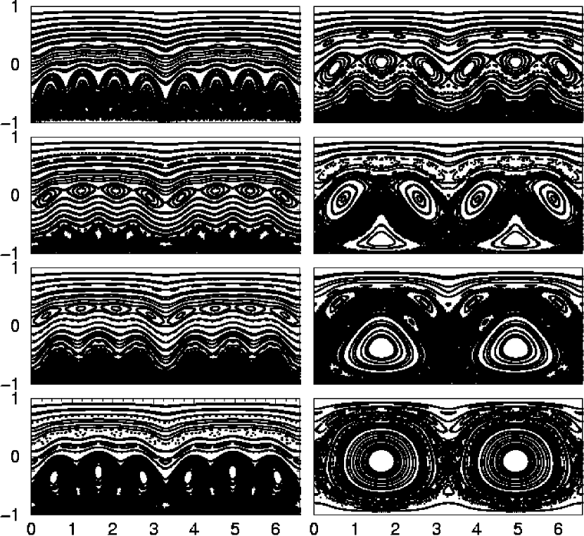
Figure 3.1: Birkhoff phase space portraits of the interior ellipse (strong eccentricity $0.8$, area $\mathrsfs{A}=\pi$), for different values of the cyclotron radius $\rho=0.40,0.44,0.50,0.54$ (left column, top to bottom) and $\rho=0.6,1.0,2.0,10.0$ (right column, top to bottom). The motion turns (more) regular as the limit of a strong field, $\rho\to 0$, and a vanishing field, $\rho\to\infty$, is approached. [figure quality reduced]

3.2.2 Integrable and hyperbolic billiards

In the field free case the ellipse is known to be the only smooth and simply connected billiard with two integrals of motion (including the circle as a special case). At finite magnetic fields, the ellipse turns chaotic, as we have just seen, except for the circle billiard. The latter exhibits the canonical angular momentum (2.12) as the second integral of the motion (provided the circle is centered at the origin of the symmetric gauge). This suggests that circular shapes, ie, the disk and the annular billiard, are the only boundaries which yield integrable motion in the magnetic field.

The other extreme type of motion is called hyperbolic, or displaying hard chaos. It is present if the stable part of phase space has zero measure rendering almost all trajectories unstable. Hyperbolic billiards are popular, although they form a small class. Early examples of field-free billiards displaying hard chaos were given by Sinai [58] and Bunimovich [59]. Conditions for the instability of orbits in magnetic billiards are discussed in [53, 54, 55]. In his recent work [14] Gutkin applied a general hyperbolicity criterion [64] to construct classes of hyperbolic magnetic billiards. The critical parameter in these sets is given by the sum of the reciprocal cyclotron radius and the (local) curvature of the boundary. Hard chaos is guaranteed in these cases only for cyclotron radii above a certain minimal value. Most of the billiards studied numerically in this report are hyperbolic at zero field, but assume a mixed chaotic phase space at any finite cyclotron radius. An example of a billiard shape which generates truly hyperbolic motion even at fairly strong fields is given in the right part of Fig. 5.1.

Since the above statements apply equally to the interior and the exterior dynamics there was no need to distinguish between them. We now turn to the question of how the classical interior and exterior problems are related.

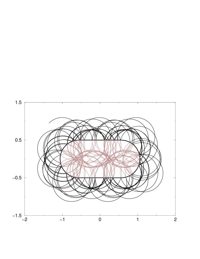
Figure 3.2: Parts of dual trajectories in the interior and exterior of a stadium-billiard at $\rho=0.5$ (sequence of 75 reflections). The billiard shape is defined in Fig. 8.5.

3.2.3 The classical interior-exterior duality

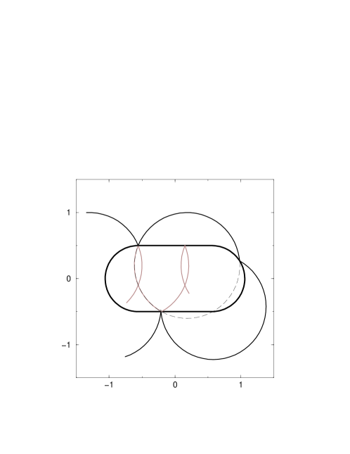
Figure 3.3: Breakdown of the duality in segments of partially corresponding trajectories (stadium of Fig. 3.2 at $\rho=0.8$.) Only the two left (top) arcs in the interior (exterior) meet with a dual partner. The breakdown occurs because a cyclotron orbit, which is obtained by continuing the arcs (dashed line) intersects the boundary more than twice.

When comparing the interior and the exterior motion the size of the cyclotron radius $\rho$ plays a crucial role. An important situation is encountered if the cyclotron radius and the billiard shape are such that any circle with radius $\rho$ intersects the boundary at most twice. For convex domains, a sufficient condition is the cyclotron radius being greater than the maximum radius of curvature, or less than the minimum radius of curvature. However, convexity is not necessary for the above condition — which we shall assume to hold for the moment.

Now consider a segment of an interior trajectory going from $\mathbf{r}(s)$ to $\mathbf{r}(s^{\prime})$. The same two points are connected by a valid exterior trajectory which travels backwards in time. Necessarily, the two arcs form a complete circle of radius $\rho$. (They do not intersect with the boundary, except at the points $\mathbf{r}(s)$ and $\mathbf{r}(s^{\prime})$, because the above criterion was assumed to hold.) The interior trajectory is reflected specularly and finally runs into the boundary at $\mathbf{r}(s^{\prime\prime})$. Clearly, the time-reversed exterior trajectory obeys the same law of specular reflection, leading to the same boundary point $\mathbf{r}(s^{\prime\prime})$. It follows that the interior dynamics and the time-reversed exterior one are described by the same Poicaré surface of section. Every interior trajectory is linked with a dual exterior trajectory, which travels backwards in time. We call this property the classical duality of interior and exterior motion. Pairs of dual trajectories are displayed in Figure 3.2 and 9.8.

As an immediate consequence of the classical duality one finds for any given interior periodic orbit a dual periodic orbit in the exterior, and vice versa. Being periodic, both may now be thought of as running forward in time, but then with opposite orders in the sequence of reflection points. Clearly, these dual partners are intimately related. We will see that they have the same stability properties and that the sum of their actions is an integer multiple of the action of a full cyclotron orbit (with the integer given by the number of reflections). Examples of dual periodic orbits are given in Figure 9.8.

Figure 3.3 shows that the duality breaks down once the duality condition that “any circle of radius $\rho$ intersects the boundary at most twice” is no longer fulfilled. Typically, only a small fraction of the phase space corresponds to arcs which violate the duality condition. Fig 3.4 gives an impression of the fraction of phase space belonging to arcs whose extension intersects the boundary more than twice.

\psfrag{rho}{$\rho$}\includegraphics[width=346.89731pt]{figs/ncfrac.eps}

Figure 3.4: Fraction of the complete interior phase space belonging to arcs which violate the duality criterion, as a function of the cyclotron radius $\rho$. (Calculated for the stadium billiard in Fig. 3.2; the squares indicate the error of the statistical sampling.)

3.3 Quantum billiards

An early study of a magnetic quantum billiard was carried out by Nakamura and Thomas [65] (see [66] for a correction). Later works are concerned with the spectral implications of the absence of time-reversal invariance [67, 68, 69]. Special geometries, such as the disk [70, 71] or, more recently, the square [72, 73], received attention as well. All these studies were limited to the first few hundred eigenvalues, and only to the interior problem.

3.3.1 General boundary conditions

The mentioned works use Dirichlet boundary conditions, ie, demand the wave function to vanish on the boundary. It is the natural choice from a physical point of view, which takes the boundary as due to an infinite potential wall. However, it will prove worthwhile to consider slightly more general, “mixed” boundary conditions which include the Dirichlet choice as a special case. They are defined by the equation

$$\psi(\mathbf{r})=\pm\frac{\lambda}{b}\big{(}\partial_{n/b}\psi(\mathbf{r})-\mathrm{i}\tilde{A}_{n}(\mathbf{r})\psi(\mathbf{r})\big{)},\quad\mathbf{r}\in\Gamma\ .$$ (3.6)

The lower sign stands for exterior problem and the symbols $\partial_{n/b}:=b\hat{\mathbf{n}}(\mathbf{r}){\boldsymbol{\nabla}}_{\!r}$ and $\tilde{A}_{n}=\hat{\mathbf{n}}(\mathbf{r})\tilde{\mathbf{A}}$ denote the scaled normal derivative and the normal component of the scaled vector potential, respectively.

The “mixing” parameter $\lambda$ interpolates between the two extremes, Dirichlet, $\lambda=0$, and Neumann boundary conditions, $\lambda^{-1}=0$. In principle, $\lambda$ may be a function of the position on the boundary, but will be assumed constant throughout. At non-vanishing $\lambda$ our boundary conditions (3.6) are the gauge-invariant generalization of the mixed boundary conditions known for the Helmholtz problem [74, 75, 76]. They imply that the normal component of the current density $\tilde{\jmath}_{n}={\rm Im}(\psi^{*}\partial_{n/b}\psi)-\tilde{A}_{n}|\psi|^{2}$ vanishes for any $\lambda$. (Take the imaginary part after multiplying (3.6) with $\psi^{*}$.) The resulting conservation of the probability density explains why the condition (3.6) keeps the problem self-adjoint for any $\lambda$. The explicit appearance of the vector potential in (3.6) is needed to ensure the gauge-invariance of the boundary conditions. The fact that the definition does not depend on the gauge freedom $\chi$ is easily seen observing the gauge dependence of a general wave function (2.31). Finally, note that $\lambda$ has the dimension of a length, cancelling the dimensionality introduced by the normal derivative. The magnitude of the latter depends on the modulus $k=\sqrt{2m_{e}E}/\hbar$ of the wave vector. To account for this trivial energy dependence of the eigenstates on the boundary condition it will be convenient (later in the semiclassical treatment) to use the dimensionless mixing parameter

$$\Lambda:=k\lambda=2\sqrt{\nu}\,\frac{\lambda}{b}\ .$$ (3.7)

We did not state the definition (3.6) of the boundary condition in terms of $\Lambda$ because its dependence on the spectral variable $\nu$ would destroy the self-adjointness of the problem rendering different eigenstates non-orthogonal.

A quite different type of boundary conditions for magnetic billiards was proposed recently by Akkermans et al. [77]. It was designed specifically to be sensitive on the “chirality” of the wave functions. For the special situation of a separable problem (disk billiard) they allow to split the interior eigenspace into two subspaces with definite chirality. We will see that this is quite close to the desired separation into bulk and edge states. However, it cannot be generalized to billiards with arbitrary shapes, and the resulting spectrum has no relation to the standard Dirichlet problem. Below, we take a different approach to separate edge and bulk, by adjusting the spectral measure according to our needs, rather than modifying the spectrum.

3.3.2 The quantum spectrum

Unlike their field-free relatives, magnetic quantum billiards offer two independent external parameters – the cyclotron radius and the magnetic length. As discussed in Section 2.3, one must specify which one is to be fixed in order to define a quantum spectrum. In the main part of this report the formulas for spectral densities are constructed at a fixed magnetic length $b$. This is done to avoid clumsy notation (and to minimize the danger of confusion). A summary of formulas for spectra defined in the semiclassical direction is given in Appendix A.7. Still, some of the numerical investigations presented below are carried out on spectra defined in the semiclassical direction, which will be clearly indicated.

The simplest function to characterize a spectrum is the spectral staircase (or number counting function) which gives the number of spectral points below the specified energy. For a set of eigenvalues $\{\nu_{n}\}$ it is formally defined as a sum

$${\rm N}(\nu):=\sum_{n=1}^{\infty}\Theta\big{(}\nu-\nu_{n}\big{)}$$ (3.8)

over Heaviside step functions $\Theta$. Note that ${\rm N}(\nu)$ is a well-defined function only for the interior problem, due to the infinite number of exterior bulk states close to each Landau level. The spectral density is conveniently defined as the energy derivative of the counting function,

$$d(\nu):=\frac{\mathrm{d}}{\mathrm{d}\nu}{\rm N}(\nu)=\sum_{n=1}^{\infty}\delta(\nu-\nu_{n})\ ,$$ (3.9)

and should be understood in the sense of distributions. Formally, such a sum of Dirac $\delta$-functions could be defined for the exterior problem as well. However, this density would be meaningful at most in a local sense since the convolution with a test function would diverge at all the Landau energies. Therefore, the following discussion of the smooth, asymptotic properties of magnetic spectra must be restricted to the interior problem.

3.3.3 Asymptotic counting functions

The spectral staircase is described asymptotically by the mean number counting function $\overline{{\rm N}}(\nu)$, which is uniquely defined [78]. For Dirichlet boundary conditions it is given by the asymptotic expression [79]

$$\overline{{\rm N}}(\nu)= \frac{\mathrsfs{A}}{b^{2}\pi}\,\nu-\frac{\mathrsfs{L}}{2\pi b}\,\nu^{\frac{1}{2}}+\frac{1}{6}+\mathord{\mathrm{O}}\big{(}\nu^{-{\frac{1}{2}}}\big{)}\ .$$ (3.10)

The expression includes only geometric quantities and the conventional wave vector $\sqrt{2m_{e}E}/\hbar=2\sqrt{\nu}/b$, which are all independent of the magnetic field. The field independence of the leading order term follows immediately from Weyl’s law, as discussed below. However, it is not obvious that the next two orders are identical to the field free case as well. This was proved only recently in [79], and for circular billiards in [80].

Note the hierarchy of the geometric quantities appearing in (3.10). The leading and the second term are proportional to the area and the circumference, respectively. The constant is determined by the mean curvature $\int_{\Gamma}\kappa(s)\mathrm{d}s=2\pi$. Moreover, the higher order terms are typically proportional to higher moments of the curvature [81]. This hierarchy reflects the systematic method to derive the boundary corrections to asymptotic quantities (see eg. [75]): The boundary is locally approximated first by a by a straight line, then a circular arc, and so on.

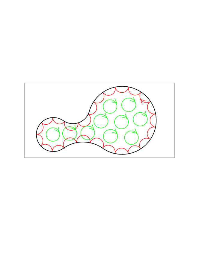
Figure 3.5: At strong magnetic fields, $\rho\ll\mathrsfs{L}$, the major part of the available phase space consists of complete cyclotron orbits. The skipping orbits give rise to a net current along the boundary. It has a counter-clockwise sense of orientation, in contrast to the cyclotron orbits.

Weyl’s law revisited

Let us consider Weyl’s law more explicitely. It states that the number of quantum states below a given energy is determined, to leading order, by the volume of phase space, within the energy shell, divided by (a power of) Planck’s quantum

$$\overline{{\rm N}}_{\rm tot}(\rho^{2},b^{2}) =\frac{1}{(2\pi\hbar)^{2}}\int\!\!\!\int\Theta(E-\mathrm{H})\,\mathrm{d}^{2}\mathbf{r}\,\mathrm{d}^{2}\mathbf{p}$$ (3.11)

$$=\frac{1}{(b^{2}\pi)^{2}}\int\!\!\!\int\Theta\big{(}\rho^{2}-|\boldsymbol{\rho}^{\prime}|^{2}\big{)}\,\mathrm{d}^{2}\mathbf{c}\,\mathrm{d}^{2}\!\boldsymbol{\rho}^{\prime}\ .$$ (3.11a)

This is the first term in the asymptotic expansion (3.10). Changing the integration of the canonical momentum to the velocity vector in the first line renders the phase space integral independent of the magnetic field (since the Jacobian is constant [82]). This shows immediately that the leading order term of the counting function (like any quantity which may be written as a phase space integral of position and velocity) cannot depend on the field strength. In (3.11a), however, we transformed the variables of integration to the radius vector $\boldsymbol{\rho}^{\prime}$, cf eq (2.7), and the cyclotron center $\mathbf{c}=\mathbf{r}-\boldsymbol{\rho}^{\prime}$, which do depend on the magnetic field. As a result, the role of Planck’s quantum is now played by the area $b^{2}\pi$. This second form of the phase space integral has the advantage that it permits to separate the volumes of skipping and cyclotron motion. The center $\mathbf{c}$ is a constant of the motion for all cyclotron orbits. Hence, integrating only the cyclotron part of the centers one obtains the area $\mathrsfs{A}_{\rm cyc}(\rho)$ of the set of points in $\mathcal{D}$ with a distance from the boundary greater than $\rho$. Consequently, the number of quantum states which correspond to cyclotron motion is given, to leading order, by the integral

$$\overline{{\rm N}}_{\rm cyc}(\rho^{2},b^{2})=\frac{2\pi}{(b^{2}\pi)^{2}}\int_{0}^{\rho}\mathrsfs{A}_{\rm cyc}(\rho^{\prime})\rho^{\prime}\mathrm{d}\rho^{\prime}\ .$$ (3.12)

We note from (3.10) that the total number of states reads to leading order,

$$\overline{{\rm N}}_{\rm tot}(\rho^{2},b^{2})=\frac{2\pi}{(b^{2}\pi)^{2}}\frac{\rho^{2}\mathrsfs{A}}{2}\ .$$ (3.13)

Hence, the number of states associated with the skipping part of phase space can be written as an integral

$$\overline{{\rm N}}_{\rm skip}(\rho^{2},b^{2})=\overline{{\rm N}}_{\rm tot}-\overline{{\rm N}}_{\rm cyc}=\frac{2\pi}{(b^{2}\pi)^{2}}\int_{0}^{\rho}\mathrsfs{A}_{\rm skip}(\rho^{\prime})\rho^{\prime}\mathrm{d}\rho^{\prime}\ ,$$ (3.14)

involving the area $\mathrsfs{A}_{\rm skip}(\rho):=\mathrsfs{A}-\mathrsfs{A}_{\rm cyc}(\rho)$. By definition, this area is given by those points in the interior domain which are closer to the boundary than the cyclotron radius, cf Fig. 3.6. It determines the mean density of those states, which correspond to the skipping part of phase space.

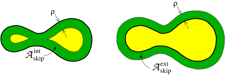
Figure 3.6: The dark shaded region indicates the area determining the phase space volume of interior (left) and exterior (right) skipping orbits. It is given by those points of the interior and exterior domain, respectively, which have a distance less than one cyclotron radius $\rho$ to the boundary.

$$\overline{d}_{\rm skip}(\nu)=\frac{\mathrm{d}}{\mathrm{d}\nu}\overline{{\rm N}}_{\rm skip}(\nu\,b^{2},b^{2})=\frac{\mathrsfs{A}_{\rm skip}(b\sqrt{\nu})}{b^{2}\pi}$$ (3.15)

This is a remarkably simple and intuitive formula. It should be made clear, however, that we do not yet have a criterion at our disposal, which provides a clear distinction of edge and bulk states. Clearly, a reasonable definition should pass the requirement of being consistent with (3.15).

Furthermore, a proper “density of edge states” will have to be well-defined also in the exterior. Let us therefore comment on the expected mean number of exterior states which correspond to skipping motion. By symmetry, it should be determined by the area $\mathrsfs{A}_{\rm skip}^{\rm ext}$ of those points in the exterior domain which are closer to the boundary than $\rho$. This can be confirmed for the circular geometry, where the integral over the skipping part of phase space in (3.11a) can be performed explicitely. For a disk of radius $R$ one obtains

$$\overline{{\rm N}}^{\rm int}_{\rm skip} =\begin{cases}\displaystyle\frac{4}{3}\,\frac{\mathrsfs{L}}{2\pi b}\,\nu^{\frac{3}{2}}-{\frac{1}{2}}\nu^{2}&\text{if $\sqrt{\nu}\,b<R$}\\[6.45831pt] \displaystyle\frac{\mathrsfs{A}}{b^{2}\pi}\nu&\text{if $\sqrt{\nu}\,b>R$}\end{cases}$$ (3.16)

$$\overline{{\rm N}}^{\rm ext}_{\rm skip} =\;\;\;\frac{4}{3}\,\frac{\mathrsfs{L}}{2\pi b}\,\nu^{\frac{3}{2}}+{\frac{1}{2}}\nu^{2}\ ,$$ (3.17)

for the interior and the exterior problem, respectively. Note that the interior number is determined by the area $\mathrsfs{A}$ of the domain once the cyclotron radius $\rho=\sqrt{\nu}\,b$ exceeds the radius $R$ of the disk, preventing any cyclotron orbits in the interior.

At very strong fields, $b\ll\rho\ll\mathrsfs{L}$, in contrast, it is the circumference term which dominates. Since in this case we may neglect the mean curvature, the average number of skipping states is approximately given by

$$\overline{{\rm N}}_{\rm skip}=\frac{4}{3}\,\frac{\mathrsfs{L}}{2\pi b}\,\nu^{\frac{3}{2}}\ .$$ (3.18)

This expression coincides with the phase space estimate for a straight line with periodic boundary conditions (see Appendix A.6).

Let us turn to another quantity which serves to characterize interior magnetic billiards — the orbital magnetism which measures the response of the spectrum to changes in the magnetic field. Its asymptotic properties may be related to a phase space integral as well.

3.4 Orbital magnetism

Employing the notion of orbital magnetism we slightly abuse a thermodynamic concept for our one-particle problem. Nonetheless, it is worthwhile to ask for the magnetic response of the billiard dynamics in the sense of statistical mechanics. We consider only micro-canonical ensembles (since we are not concerned with effects of finite temperature) which means that averages are performed on the energy shell in phase space, ie, among all orbits of a given cyclotron radius.

Let us first consider the classical motion along a single periodic trajectory. Being charged the particle constitutes an electric current which in turn induces a magnetic moment. Will it serve to strengthen or to weaken the applied magnetic field? Clearly, the latter is expected in the case of a cyclotron orbit. Here, the (scaled) magnetic moment turns negative,

$${\frac{1}{2}}\int_{0}^{\widetilde{T}_{\rm cyc}}\!\tilde{\mathbf{r}}({\tilde{t}})\times\tilde{\mathbf{v}}({\tilde{t}})\,\mathrm{d}{\tilde{t}}=-\nu\ ,$$ (3.19)

which shows that the cyclotron part of phase space is diamagnetic. The skipping orbits, on the other hand, will in general give rise to both signs. At strong fields (if the cyclotron radius is shorter than the minimum diameter of the billiard) skipping trajectories carry a net current along the boundary. It is orientated clockwise, ie, opposite to the cyclotron orbits (see Fig. 3.5). A detailed analysis [83] shows that, in any case, a subtle cancellation mechanism between cyclotron and skipping orbits is at work, which guarantees that classically there is no net orbital magnetization. This is the van Leeuwen theorem [83, 82].

The statement is proved immediately by evoking the thermodynamic definition of the magnetization as the derivative of a thermodynamic potential (the free energy or the grand canonical potential) with respect to the magnetic field. The potentials are determined by the partition sum, which is a phase space integral in the classical case. As such it cannot depend on the magnetic field for the reasons given in the preceding section [82].

Before we turn to the precise quantum definition it should be emphasized that orbital magnetism in its proper sense is an effect of many particles at finite temperature. Assuming the temperature to be much larger than the spacing between Landau levels, $T\gg\hbar\omega_{c}/k_{B}$, Landau showed [19] that a degenerate Fermi gas exhibits a small net diamagnetic response. This Landau diamagnetism is an effect of the bulk. Asymptotic corrections due to the existence of a boundary are discussed in [85, 86, 87, 79, 88, 80]. Recently, the effect met some renewed interest since the geometry of mesoscopic devices may greatly enhance orbital magnetism. Semiclassical treatments in terms of periodic orbit theory may be found in [89, 90, 91, 72, 92]. In these works the magnetic field was assumed to be very weak such that the bending of the trajectories could be neglected. An exception is the study of the quantum and semiclassical magnetization of the magnetic disk in [93]. A comprehensive review on the subject of orbital magnetism is given in [94].

In the following we shall use the concept of orbital magnetization merely as a means of characterizing magnetic billiards. We shall argue that it is advantageous to adopt a modified definition of orbital magnetization. In order to motivate this we start with the conventional one.

Conventional magnetization

Given the spectrum $\{E_{n}\}$ at finite magnetic field $B$ one may conventionally define the magnetization as

$$\mathcal{M}_{\rm conv}(E,B):= -\!\!\!\sum_{E_{n}\leq E}\frac{\mathrm{d}E_{n}}{\mathrm{d}B}=\int_{0}^{E}\!\!\!{\rm m}(E^{\prime};B)\,\mathrm{d}E^{\prime}\ .$$ (3.20)

This is the one-particle and zero-temperature limit of the standard thermodynamic definition. By means of equation (3.20) the function ${\rm m}(E,B)$ is introduced which we call the magnetization density,

$${\rm m}(E,B):= \frac{\mathrm{d}{{\rm N}}_{\rm tot}}{\mathrm{d}B}(E,B)=\,-\sum_{n}\frac{\mathrm{d}E_{n}}{\mathrm{d}B}\,\delta(E-E_{n})\ .$$ (3.21)

The relation of ${\rm m}(E,B)$ to the electrodynamic interpretation of the magnetization is seen once we note the derivative of the Hamilton operator (2.8) with respect to the magnetic field,

$$\frac{\mathrm{d}\mathrm{H}}{\mathrm{d}B}=-\frac{q}{2}\,(\mathbf{r}\times\mathbf{v})_{\rm sym}\ .$$ (3.22)

It is the operator of the magnetic moment, where $(\cdot)_{\rm sym}$ indicates the symmetrized form. It follows that the energy derivatives ${\mathrm{d}E_{n}}/{\mathrm{d}B}$ in eq (3.21) are given by the corresponding expectation values of the magnetic moment, ie, the magnetization density (3.21) reads

$${\rm m}(E,B)=\sum_{n}\frac{q}{2}\langle\psi_{n}|(\mathbf{r}\times\mathbf{v})_{\rm sym}|\psi_{n}\rangle\,\delta(E-E_{n})\ .$$ (3.23)

The fact that the mean magnetization (density) vanishes follows immediately from the field-independence of $\overline{{\rm N}}$ (3.10), as noted above. At strong fields the negative moments of (many) bulk states are balanced, consequently, by the large, positive magnetic moments of relatively few edge states. This is seen much more clearly once we modify the definition of the magnetization such that is complies with the scaling properties of the system.

Bulk and edge magnetization

We proceed to define a scaled magnetization which has considerable advantages compared to the conventional one. According to (2.37) the spectrum $\{\nu_{n}\}$ depends parametrically on the magnetic length, $\nu_{n}=\nu_{n}(b^{2})$. It is natural to define the scaled magnetization density such that it yields the density of the scaled magnetic moment (3.25), in analogy to (3.23). Hence, one is led to the definition

$$\widetilde{{\rm m}}(\nu,b^{2}):=\sum_{n}{\frac{1}{2}}\langle\psi_{n}|(\tilde{\mathbf{r}}\times\tilde{\mathbf{v}})_{\rm sym}|\psi_{n}\rangle\,\delta(\nu-\nu_{n})\ .$$ (3.24)

From the explicit form of the scaled Hamiltonian one can easily show that

$${\frac{1}{2}}\langle\psi_{n}|(\tilde{\mathbf{r}}\times\tilde{\mathbf{v}})_{\rm sym}|\psi_{n}\rangle=b^{2}\frac{\mathrm{d}\nu_{n}}{\mathrm{d}b^{2}}-\nu_{n}\ .$$ (3.25)

Thus, the scaled magnetization density can be written in terms of derivatives of the number counting function,

$$\widetilde{{\rm m}}(\nu,b^{2})=\sum_{n}\Big{(}b^{2}\frac{\mathrm{d}\nu_{n}}{\mathrm{d}b^{2}}-\nu_{n}\Big{)}\,\delta(\nu-\nu_{n})=-b^{2}\frac{\partial{\rm N}}{\partial b^{2}}-\nu\frac{\partial{\rm N}}{\partial\nu}\ .$$ (3.26)

The scaled magnetization follows by integrating the density.

$$\widetilde{\mathcal{M}}(\nu,b^{2}):= \,\int_{0}^{\nu}\!\!\widetilde{{\rm m}}(\nu^{\prime},b^{2})\,\mathrm{d}\nu^{\prime}=\sum_{\nu_{n}\leq\nu}\Big{(}b^{2}\frac{\mathrm{d}\nu_{n}}{\mathrm{d}b^{2}}-\nu_{n}\Big{)}$$ (3.27)

$$= \,\widetilde{\mathcal{M}}_{\rm edge}+\widetilde{\mathcal{M}}_{\rm bulk}$$ (3.27a)

As indicated in the second line the scaled magnetization splits up naturally into two parts which we call, respectively, the edge magnetization,

$$\widetilde{\mathcal{M}}_{\rm edge}(\nu,b^{2}) :=\sum_{\nu_{n}\leq\nu}b^{2}\frac{\mathrm{d}\nu_{n}}{\mathrm{d}b^{2}}=-\int_{0}^{\nu}b^{2}\frac{\mathrm{d}}{\mathrm{d}b^{2}}{\rm N}(\nu^{\prime},b^{2})\,\mathrm{d}\nu^{\prime}\ ,$$ (3.28)

and the bulk magnetization,

$$\widetilde{\mathcal{M}}_{\rm bulk}(\nu,b^{2}) :=-\sum_{\nu_{n}\leq\nu}\nu_{n}=-\int_{0}^{\nu}\nu^{\prime}\frac{\mathrm{d}}{\mathrm{d}\nu^{\prime}}{\rm N}(\nu^{\prime},b^{2})\,\mathrm{d}\nu^{\prime}\ .$$ (3.29)

This naming is appropriate since any Landau state (2.19) exhibits a scaled magnetic moment $\langle n,m|{\frac{1}{2}}(\tilde{\mathbf{r}}\times\tilde{\mathbf{v}})_{\rm sym}|n,m\rangle=-(n+{\frac{1}{2}})=-\nu$, like the classical cyclotron orbit (3.19). Each eigenstate contributes to both magnetization densities,

$$\widetilde{{\rm m}}_{\rm edge}(\nu,b^{2}) =\sum_{n}b^{2}\frac{\mathrm{d}\nu_{n}}{\mathrm{d}b^{2}}\,\delta(\nu-\nu_{n})$$ (3.30)

and

$$\widetilde{{\rm m}}_{\rm bulk}(\nu,b^{2}) =-\sum_{n}\nu_{n}\,\delta(\nu-\nu_{n})\ .$$ (3.31)

The energies of bulk states lie close to the Landau levels and the nearer they get to the level the less they depend on $b^{2}$ (since the Landau energy is independent of $b^{2}$). Hence, they give rise to a negligible edge contribution. Edge states, in contrast, contribute to the edge magnetization much stronger than to the bulk. This follows from the mean values of the magnetization. For the smooth edge magnetization density one finds, cf (3.10),

$$\overline{{\rm m}}_{\rm edge}(\nu,b^{2})=-b^{2}\frac{\partial\overline{{\rm N}}}{\partial b^{2}}=\frac{\mathrsfs{A}}{b^{2}\pi}\nu-{\frac{1}{2}}\frac{\mathrsfs{L}}{2\pi b}\nu^{\frac{1}{2}}\ .$$ (3.32)

Remarkably, the bulk mean value assumes a form,

$$\overline{{\rm m}}_{\rm bulk}(\nu,b^{2})=-\nu\frac{\partial\overline{{\rm N}}}{\partial\nu}(\nu,b^{2})=-\frac{\mathrsfs{A}}{b^{2}\pi}\nu+{\frac{1}{2}}\frac{\mathrsfs{L}}{2\pi b}\nu^{\frac{1}{2}}\ ,$$ (3.33)

which cancels the mean edge magnetization identically. Hence, the mean (total) magnetization, $\overline{\mathcal{M}}=\overline{\mathcal{M}}_{\rm edge}+\overline{\mathcal{M}}_{\rm bulk}$ vanishes like in the conventional case. This holds strictly for any field, independently of whether or not there is a classical separation into skipping and cyclotron orbits.

The edge magnetization (3.28) defined in this section embodies a first quantity which allows to distinguish edge states quantitatively. It gives the excess magnetization of the states which arises due to the existence of a boundary, ie, as compared to the expected diamagnetism of a state in the infinite plane.

4 Quantization in the interior and the exterior: The boundary integral method

In the present chapter, we show how to solve the quantization problem for interior and exterior magnetic billiards by means of a boundary integral method. It provides the spectra and wave functions of arbitrarily shaped billiard domains, and includes the general boundary conditions discussed in Section 3.3.1. Moreover, the boundary integral formalism constitutes the basis for the semiclassical theory discussed in Chapter 6.

4.1 Boundary methods

As compared to the field free case, it is surprisingly difficult to obtain the quantum spectra of magnetic billiards. So far, numerical studies were restricted to the interior problem and performed almost exclusively by diagonalizing the Hamiltonian[65, 67, 68, 69, 95]. This requires the choice and truncation of a basis, which is problematic for general billiards, where no natural magnetic basis set exists. Consequently, results were limited to the first few hundred eigenvalues.

In the case of field free billiards quantum spectra are usually obtained by transforming the eigenvalue problem into an integral equation of lower dimension. The corresponding integral operator is defined in terms of the free Green function, and depends only on the boundary [96, 97, 98, 99, 100, 101]. This method is known to be more efficient than diagonalization by an order of magnitude [102, 103]. We proceed to extend these ideas to magnetic billiards. A step in this direction was taken by Tiago et al.[33], who essentially propose a null-field method [104] for (interior) magnetic billiards. It involves the irregular Green function (A.1) in angular momentum decomposition. A drawback of the approach is that this function must be known for large angular momenta, which turns out to be numerically impractical. Moreover, the method does not apply for the exterior problem.

In the following we derive the boundary integral method for magnetic billiards. Like in the field free case, it involves the regular Green function in position space representation. We present the method for the interior and the exterior problem, and general boundary conditions.

4.2 The boundary integral equations

4.2.1 Single and double layer equations

The stationary eigenfunction of a magnetic billiard at energy $\nu$ is defined by the differential equation

$$\left({\tfrac{1}{2}}\big{(}-\mathrm{i}{\boldsymbol{\nabla}}_{\!r/b}-\tilde{\mathbf{A}}(\mathbf{r})\big{)}^{2}-2\nu\right)\psi(\mathbf{r})=0\ ,$$ (4.1)

and a specification of the wave function on the billiard boundary $\Gamma$. The free Green function, ${\rm G}_{\nu}$, was shown to satisfy the inhomogeneous Schrödinger equation

$$\left(\tfrac{1}{2}\big{(}-\mathrm{i}{\boldsymbol{\nabla}}_{\!r/b}-\tilde{\mathbf{A}}(\mathbf{r})\big{)}^{2}-2\nu\right){\rm G}_{\nu}(\mathbf{r};\mathbf{r}_{0})=-\tfrac{1}{2}\,\delta\!\left(\frac{\mathbf{r}-\mathbf{r}_{0}}{b}\right)\ .$$ (4.2)

Our goal is to cast the quantization problem into an integral equation defined on the billiard boundary. To that end, we take the complex conjugate of (4.1) and multiply it (from the left) with ${\rm G}_{\nu}$. Similarly, equation (4.2) is multiplied with $\psi^{*}$ and subtracted from the former expression. One obtains an equation

$$\psi^{*}\,{\boldsymbol{\nabla}}_{\!r/b}^{2}{\rm G}_{\nu}-{\rm G}_{\nu}\,{\boldsymbol{\nabla}}_{\!r/b}^{2}\psi^{*}-2\mathrm{i}\,{\boldsymbol{\nabla}}_{\!r/b}\big{(}\tilde{\mathbf{A}}\psi^{*}{\rm G}_{\nu}\big{)}=\psi^{*}\,\delta\!\left(\frac{\mathbf{r}-\mathbf{r}_{0}}{b}\right)\ ,$$ (4.3)

which has a form suitable for the Green and Gauss integral theorems. It holds everywhere in the plane, except for the boundary $\Gamma$, where the boundary condition (3.6) introduces a discontinuity in the derivative of $\psi$.

We start by considering the interior problem and sketch the treatment of the exterior case afterwards. Choosing the initial point of the Green function away from the boundary, $\mathbf{r}_{0}\in\mathbb{R}^{2}\setminus\Gamma$, the integral of (4.3) over the (interior) domain $\mathcal{D}$ may be transformed to a line integral,

$$\int_{\Gamma}\big{[}\psi^{*}\,(\partial_{n/b}{\rm G}_{\nu}-\mathrm{i}\,\tilde{A}_{n}\,{\rm G}_{\nu})-{\rm G}_{\nu}\,(\partial_{n/b}\psi^{*}+\mathrm{i}\,\tilde{A}_{n}\,\psi^{*})\big{]}\frac{{\rm d}\Gamma}{b}\\ =\begin{cases}\psi^{*}(\mathbf{r}_{0})&\text{if $\mathbf{r}_{0}\in\smash{\stackrel{{{}_{\circ}}}{{\mathcal{D}}}}$ }\\ 0&\text{if $\mathbf{r}_{0}\in\mathbb{R}^{2}\setminus{\mathcal{D}}$. }\end{cases}$$ (4.4)

It is defined on the boundary $\Gamma$ (with the normal components of the vector potential and the gradient denoted as $\tilde{A}_{n}=\hat{\mathbf{n}}(\mathbf{r})\tilde{\mathbf{A}}$ and $\partial_{n/b}:=b\hat{\mathbf{n}}(\mathbf{r}){\boldsymbol{\nabla}}_{\!r}$, respectively). Note that the vector potential part of the integrand was split which is necessary for a gauge invariant formulation of the integral equations.

The single layer equations

We choose $\mathbf{r}_{0}\in\Gamma$ and define $\mathbf{r}_{0}^{\pm}:=\mathbf{r}_{0}\pm\varepsilon\hat{\mathbf{n}}_{0}$, for small $\varepsilon>0$. By adding the two equations in (4.4), one obtains

$$\int_{\Gamma}\big{[}\psi^{*}\,({\partial}_{n/b}{\rm G}_{\nu}^{{}^{\scriptstyle\varepsilon}}-\mathrm{i}\,\tilde{A}_{n}\,{\rm G}_{\nu}^{{}^{\scriptstyle\varepsilon}})-{\rm G}_{\nu}^{{}^{\scriptstyle\varepsilon}}\,(\partial_{n/b}\psi^{*}+\mathrm{i}\,\tilde{A}_{n}\,\psi^{*}))\big{]}\frac{{\rm d}\Gamma}{b}={\tfrac{1}{2}}\psi^{*}(\mathbf{r}_{0}^{-})\ .$$ (4.5)

Here, we used the abbreviation ${\rm G}_{\nu}^{{}^{\scriptstyle\varepsilon}}={\tfrac{1}{2}}{\rm G}_{\nu}(\mathbf{r};\mathbf{r}_{0}^{+})+{\tfrac{1}{2}}{\rm G}_{\nu}(\mathbf{r};\mathbf{r}_{0}^{-})$. Equation (4.5) holds for all (sufficiently small) $\varepsilon>0$, hence the limit $\varepsilon\to 0$ exists. Moreover, observing the asymptotic properties of the Green function (cf Sect. 2.5.3), it can be shown, that the integration and the limit ${\rm G}_{\nu}^{{}^{\scriptstyle\varepsilon}}\to{\rm G}_{\nu}$, ${\partial}_{n/b}{\rm G}_{\nu}^{{}^{\scriptstyle\varepsilon}}\to\partial_{n/b}{\rm G}_{\nu}$ may be interchanged. Inserting the boundary condition (3.6) we obtain, after renaming the limiting function $u=\partial_{n/b}\psi^{*}+\mathrm{i}\tilde{A}_{n}\psi^{*}$, $u_{0}:=u(\mathbf{r}_{0})$,

$$\int_{\Gamma}\big{[}\,{\rm G}_{\nu}-\frac{\lambda}{b}(\partial_{n/b}{\rm G}_{\nu}-\mathrm{i}\,\tilde{A}_{n}\,{\rm G}_{\nu})\big{]}\,u\,\frac{{\rm d}\Gamma}{b}=\frac{\lambda}{b}\,(-{\tfrac{1}{2}}u_{0})\ ,$$ (4.6)

an integral equation defined on the boundary $\Gamma$ [35].

In order to derive the corresponding equation for the exterior problem, consider a large disk $\mathcal{K}_{p}\supset\mathcal{D}$ of radius $p$, and integrate (4.3) over $\mathcal{K}_{p}\cap\smash{\stackrel{{{}_{\circ}}}{{\mathcal{D}}}}$. Once $\mathbf{r}_{0}$ lies in the vicinity of $\Gamma$, the contribution of $\partial\mathcal{K}_{p}$ to the boundary integral vanishes as $p\to\infty$, due to the exponential decay of the regular Green function ${\rm G}_{\nu}$. Similar to eq (4.5) one obtains an equation which permits the limit $\varepsilon\to 0$ to be taken before performing the integration. The resulting boundary integral equation differs from (4.6) only by a sign. In the following, we shall treat both cases simultaneously, with the convention that the upper sign stands for the interior problem, and the lower sign for the exterior one,

$$\int_{\Gamma}\big{[}\,{\rm G}_{\nu}\mp\frac{\lambda}{b}(\partial_{n/b}{\rm G}_{\nu}-\mathrm{i}\,\tilde{A}_{n}\,{\rm G}_{\nu})\big{]}\,u\,\frac{{\rm d}\Gamma}{b}=\frac{\lambda}{b}\,(-{\tfrac{1}{2}}u_{0})\ .$$ (4.7)

In analogy to the Helmholtz problem [96], we will refer to these equations as the single layer equations for the interior and the exterior domain.

The double layer equations

A second kind of boundary integral equations can be derived by applying the differential operator $(\partial_{n_{0}/b}+\mathrm{i}\tilde{A}_{n_{0}}):=\hat{\mathbf{n}}(\mathbf{r}_{0})({\boldsymbol{\nabla}}_{\!r_{0}/b}+\mathrm{i}\tilde{\mathbf{A}}(\mathbf{r}_{0})$ on equation (4.5),

$$\int_{\Gamma}\psi^{*}\,({\partial}_{n_{0}/b}+\mathrm{i}\,\tilde{A}_{n_{0}})({\partial}_{n/b}{\rm G}_{\nu}^{{}^{\scriptstyle\varepsilon}}-\mathrm{i}\,\tilde{A}_{n}\,{\rm G}_{\nu}^{{}^{\scriptstyle\varepsilon}})\frac{{\rm d}\Gamma}{b}\\ -\int_{\Gamma}({\partial}_{n_{0}/b}{\rm G}_{\nu}^{{}^{\scriptstyle\varepsilon}}+\mathrm{i}\,\tilde{A}_{n_{0}}\,{\rm G}_{\nu}^{{}^{\scriptstyle\varepsilon}})(\partial_{n/b}\psi^{*}+\mathrm{i}\tilde{A}_{n}\psi^{*})\frac{{\rm d}\Gamma}{b}\\ =\pm{\tfrac{1}{2}}(\partial_{n_{0}/b}+\mathrm{i}\,\tilde{A}_{n_{0}})\psi^{*}(\mathbf{r^{\mp}_{0}})\ .$$ (4.8)

This equation is true for all $\varepsilon>0$, which means that the limit $\varepsilon\to 0$ exists. As for the second integral, we may again permute the limit and the integration which yields a proper integral. Consequently, the limit of the first integral is finite, too. However, in the first integral we are not allowed to exchange the integration with taking the limit because the limiting integrand (4.26) has a $1/(\mathbf{r}-\mathbf{r_{0}})^{2}$-singularity which is not integrable (see below).

Integral operators of this kind are named hypersingular [105]. Similar to a Cauchy principal value integral, they are defined by taking a special limit. However, compared to the principal value the singularity is stronger by one order in the present case. Below, in Section 4.3, we define which limit is to be taken. It is denoted by ${\textstyle=\int}$ and should be read “finite part of the integral”. With this concept and equation (3.6), we obtain the double  layer equations,

$$\int_{\Gamma}(\partial_{n_{0}/b}{\rm G}_{\nu}+\mathrm{i}\,\tilde{A}_{n_{0}}\,{\rm G}_{\nu})\,u\,\frac{{\rm d}\Gamma}{b}\\ \mp\frac{\lambda}{b}=\int_{\Gamma}({\partial}_{n_{0}/b}+\mathrm{i}\,\tilde{A}_{n_{0}})({\partial}_{n/b}{\rm G}_{\nu}-\mathrm{i}\,\tilde{A}_{n}\,{\rm G}_{\nu})\,u\,\frac{{\rm d}\Gamma}{b}=\mp\tfrac{1}{2}u_{0}\ ,$$ (4.9)

which are again integral equations defined on the boundary $\Gamma$.

The spectral determinants

It is useful to introduce a set of integral operators (whose labels D and N indicate correspondence to pure Dirichlet or Neumann conditions):

$$\mathsf{Q}^{\rm D}_{\rm sl}[u] =\int_{\Gamma}\!{\rm d}\Gamma\,{\rm G}_{\nu}\,u$$ (4.10)

$$\mathsf{Q}^{\rm N}_{\rm sl}[u] =\int_{\Gamma}\!\frac{{\rm d}\Gamma}{b}(\partial_{n/b}{\rm G}_{\nu}-\mathrm{i}\,\tilde{A}_{n}\,{\rm G}_{\nu})\,u$$ (4.11)

$$\mathsf{Q}^{\rm D}_{\rm dl}[u] =\int_{\Gamma}\!\frac{{\rm d}\Gamma}{b}(\partial_{n_{0}/b}{\rm G}_{\nu}+\mathrm{i}\,\tilde{A}_{n_{0}}\,{\rm G}_{\nu})\,u$$ (4.12)

$$\mathsf{Q}^{\rm N}_{\rm dl}[u] =\,\,=\int_{\Gamma}\!\frac{{\rm d}\Gamma}{b^{2}}({\partial}_{n_{0}/b}+\mathrm{i}\tilde{A}_{n_{0}})({\partial}_{n/b}{\rm G}_{\nu}-\mathrm{i}\,\tilde{A}_{n}\,{\rm G}_{\nu})\,u$$ (4.13)

They act in the space of square-integrable periodic functions, $u\in{{\mathcal{L}_{2}}}(\Gamma)$, with the period given by the circumference $\mathrsfs{L}$.

Nontrivial solutions of the single layer equations (4.7) and double layer equations (4.9) exist for energies where the corresponding Fredholm determinants vanish,

$$\det\left[\mathsf{Q}^{\rm D}_{\rm sl}\mp\lambda\mathsf{Q}^{\rm N}_{\rm sl}+\frac{\lambda}{2}\mathsf{id}\right] =0\quad\quad\mbox{(single layer)}$$ (4.14)

$$\det\left[\mathsf{Q}^{\rm D}_{\rm dl}\mp\lambda\mathsf{Q}^{\rm N}_{\rm dl}\pm\frac{1}{2}\mathsf{id}\right] =0\quad\quad\mbox{(double layer).}$$ (4.15)

Hence, these are secular equations although the explicit dependence on the spectral variable is not shown in our abbreviated notation. However, each of the determinants (4.14) and (4.15) may have roots, which do not correspond to solutions of the original eigenvalue problem given by (4.1) and (3.6). For finite $\varepsilon$, the equations (4.5) and (4.8) are still equivalent to the latter. They acquire additional spurious solutions only as they are transformed to boundary integral equations by the limit $\varepsilon\to 0$.

4.2.2 Spurious solutions and the combined operator

The physical origin of the redundant zeros is apparent in our gauge invariant formulation: They are proper solutions for the domain complementary to the one considered. This is obvious for the single layer equation with Dirichlet boundary conditions ($\lambda=0$), where the spectral determinant does not depend on the orientation of the normals. The same is true for the double layer equation with Neumann boundary conditions ($\lambda^{-1}=0$).

In general, the character of the spurious solutions may be summarized as follows: Independently of the boundary conditions, the single layer equation includes the Dirichlet solutions of that domain which is complementary to the one considered. Likewise, the double layer equation is polluted by the Neumann solutions of the complementary domain, irrespective of the boundary conditions employed. This statement is easily proved by observing that the single-layer-Neumann operator and the double-layer-Dirichlet operator are adjoint to each other, $\mathsf{Q}^{\rm N}_{\rm sl}=(\mathsf{Q}^{\rm D}_{\rm dl})^{\dagger}$, while the operators $\mathsf{Q}^{\rm D}_{\rm sl}$ and $\mathsf{Q}^{\rm N}_{\rm dl}$ are self-adjoint (see below). Now assume that $u$ is a complementary Dirichlet solution. In Dirac notation,

$$\mathsf{Q}^{\rm D}_{\rm sl}|u\rangle=0 \quad\wedge\quad\mathsf{Q}^{\rm D}_{\rm dl}|u\rangle\mp\tfrac{1}{2}|u\rangle=0$$ (4.16)

$${\Rightarrow}\qquad\langle u|\mathsf{Q}^{\rm D}_{\rm sl}=0 \quad\wedge\quad\langle u|\mathsf{Q}^{\rm N}_{\rm sl}\mp\tfrac{1}{2}\langle u|=0\ .$$

Applying the dual of $u$ to the single layer operator yields

$$\langle u|\mathsf{Q}^{\rm D}_{\rm sl}\mp\lambda\Big{\{}\langle u|\mathsf{Q}^{\rm N}_{\rm sl}\mp\tfrac{1}{2}\langle u|\Big{\}}=0\ ,$$ (4.17)

which implies that the Fredholm determinant of the single layer operator vanishes. Similarly, if $u$ is a complementary Neumann solution,

$$\pm\mathsf{Q}^{\rm N}_{\rm sl}|u\rangle+\tfrac{1}{2}|u\rangle=0\quad\wedge\quad\mathsf{Q}^{\rm N}_{\rm dl}|u\rangle=0$$ (4.18)

$${\Rightarrow}\qquad \pm\langle u|\mathsf{Q}^{\rm D}_{\rm dl}+\tfrac{1}{2}\langle u|=0\quad\wedge\quad\langle u|\mathsf{Q}^{\rm N}_{\rm dl}=0$$

then its dual satisfies the double layer equation, again for any $\lambda$,

$$\pm\Big{\{}\pm\langle u|\mathsf{Q}^{\rm D}_{\rm dl}+\tfrac{1}{2}\langle u|\Big{\}}\mp\lambda\langle u|\mathsf{Q}^{\rm N}_{\rm dl}=0\ .$$ (4.19)

Since the spurious solutions are never of the same type, it is possible to dispose of them by requiring that both, the single and the double layer equations, should be satisfied by the same solution $u$. Therefore, one obtains a necessary and sufficient condition for the definition of the spectrum by considering a combined operator

$$\mathsf{Q}_{\rm c}^{\pm}:=\left(\mathsf{Q}^{\rm D}_{\rm dl}\mp\lambda\mathsf{Q}^{\rm N}_{\rm dl}\pm\frac{1}{2}\mathsf{id}\right)+\mathrm{i}\alpha_{\rm c}\left(\mathsf{Q}^{\rm D}_{\rm sl}\mp\lambda\mathsf{Q}^{\rm N}_{\rm sl}+\frac{\lambda}{2}\mathsf{id}\right)\ ,$$ (4.20)

with an arbitrary constant $\alpha_{\rm c}$. It has a zero eigenvalue only if both, single and double layer operators do. In practice, the spectrum is obtained by finding the roots of the spectral function

$$\xi(\nu)=\det\left[\mathsf{Q}_{\rm c}^{\pm}\right]\ .$$ (4.21)

It is worthwhile noting that (for the interior problem) spurious solutions will not appear if one uses the irregular Green function. The reason is that the gauge-independent part of this function is complex, which destroys the mutual adjointness of the operators. This is why the irregular Green function had to be chosen for the null-field method [33]. For the boundary integral method, the option to use this exponentially divergent solution of (4.2) is excluded, since the corresponding operator would get arbitrarily ill-conditioned once the diameter of the domain $\mathcal{D}$ exceeds the cyclotron diameter. The exterior problem cannot even formally be solved using ${\rm G}^{\rm(irr)}_{\nu}$ (due to an essential singularity at the origin).

A last remark is concerned with the important case of Dirichlet boundary conditions. Here, one could as well derive a pair of boundary integral equations that are not gauge-invariant. (Just set $\psi^{*}=0$ in (4.4) and consider $u=\partial_{n/b}\psi^{*}$.) Of course, these equations would yield all the proper gauge-invariant eigen-energies of the problem. However, the energies of the additional spurious solutions would depend on the chosen gauge, and a characterization of the latter in terms of solutions of a complementary problem would not be possible.

The fact that the spurious solutions can be removed by considering a combined integral operator is of great practical importance for numerical calculations [35, 106]. An individual spurious solution of the single or the double layer operator may be identified as well after evaluating the corresponding wave functions by observing in which domain it vanishes.

4.2.3 Wave functions

The eigenfunctions at points off the boundary, $\psi(\mathbf{r}_{0}\notin\Gamma)$, are determined by the null vectors $u$ corresponding to the roots of the spectral determinant. From equation (4.4) we obtain immediately an integral representation of the (un-normalized) wave function,

$$\psi(\mathbf{r}_{0})=\,\pm\bigg{[}\int_{\Gamma}\!\frac{{\rm d}\Gamma}{b}\big{[}\pm\frac{\lambda}{b}(\partial_{n/b}{\rm G}_{\nu}-\mathrm{i}\tilde{A}_{n}{\rm G}_{\nu})-{\rm G}_{\nu}\big{]}u\bigg{]}^{*}\ ,$$ (4.22)

for $\mathbf{r}_{0}\notin\Gamma$. According to eq. (4.4) the integral vanishes identically either in the interior or in the exterior. This is indeed confirmed by our numerical calculations which are reported in the next chapter.

In order to calculate the current density (2.32) one needs the gauge invariant gradient of the wave function. An integral formula is obtained from equation (4.4), after applying the differential operator ${\boldsymbol{\nabla}}_{r_{0}/b}+\mathrm{i}\tilde{\mathbf{A}}_{0}$,

$${\boldsymbol{\nabla}}_{r_{0}/b}\psi(\mathbf{r}_{0})-\mathrm{i}\tilde{\mathbf{A}}(\mathbf{r}_{0})\psi(\mathbf{r}_{0})=\,\pm\bigg{[}\int_{\Gamma}\!\frac{{\rm d}\Gamma}{b}\begin{aligned} \big{[}&\pm\frac{\lambda}{b}({\boldsymbol{\nabla}}_{r_{0}/b}+\mathrm{i}\tilde{\mathbf{A}}_{0})(\partial_{n/b}{\rm G}_{\nu}-\mathrm{i}\tilde{A}_{n}{\rm G}_{\nu})\\ &-({\boldsymbol{\nabla}}_{r_{0}/b}{\rm G}_{\nu}+\mathrm{i}\tilde{\mathbf{A}}_{0}{\rm G}_{\nu})\big{]}u\bigg{]}^{*}\ .\end{aligned}$$

The densities of other observables can be obtained by similar boundary integrals.

4.3 The boundary operators

In the following, we give explicit expressions for the boundary integrals. This allows to define the “finite part integral” appearing in the double layer equation (4.9).

The integral operators (4.10) – (4.13),

$$\big{(}\mathsf{Q}[u]\big{)}(\mathbf{r}_{0})=\int_{\Gamma}\!\mathrm{d}\Gamma\,{\rm q}(\mathbf{r};\mathbf{r}_{0})u(\mathbf{r})\ ,$$ (4.24)

are defined by their integral kernels ${\rm q}(\mathbf{r};\mathbf{r}_{0})$. The form of the Green function (2.61) leads to the expressions

$${\rm q}_{\rm sl}^{\rm D}(\mathbf{r};\mathbf{r}_{0})= \,{\rm E}(\mathbf{r};\mathbf{r}_{0})\,{\rm G}^{0}_{\nu}(z)$$ (4.25)

$${\rm q}_{\rm sl}^{\rm N}(\mathbf{r};\mathbf{r}_{0})= \,{\rm E}(\mathbf{r};\mathbf{r}_{0})\,\bigg{\{}-\mathrm{i}\frac{(\mathbf{r}-\mathbf{r}_{0})\times\hat{\mathbf{n}}}{b^{2}}\,{\rm G}^{0}_{\nu}(z)+2\frac{(\mathbf{r}-\mathbf{r}_{0})\,\hat{\mathbf{n}}}{(\mathbf{r}-\mathbf{r}_{0})^{2}}\,z\frac{\mathrm{d}}{\mathrm{d}z}{\rm G}^{0}_{\nu}(z)\bigg{\}}$$ (4.26)

$${\rm q}_{\rm dl}^{\rm D}(\mathbf{r};\mathbf{r}_{0})= \,{\rm E}(\mathbf{r};\mathbf{r}_{0})\,\bigg{\{}-\mathrm{i}\frac{(\mathbf{r}-\mathbf{r}_{0})\times\mathbf{n_{0}}}{b^{2}}\,{\rm G}^{0}_{\nu}(z)-2\frac{(\mathbf{r}-\mathbf{r}_{0})\,\hat{\mathbf{n}}_{0}}{(\mathbf{r}-\mathbf{r}_{0})^{2}}\,z\frac{\mathrm{d}}{\mathrm{d}z}{\rm G}^{0}_{\nu}(z)\bigg{\}}$$ (4.27)

$${\rm q}_{\rm dl}^{\rm N}(\mathbf{r};\mathbf{r}_{0})= \,{\rm E}(\mathbf{r};\mathbf{r}_{0})\,\bigg{\{}\left(-\frac{((\mathbf{r}-\mathbf{r}_{0})\times\hat{\mathbf{n}}_{0})((\mathbf{r}-\mathbf{r}_{0})\times\hat{\mathbf{n}})}{b^{4}}-\mathrm{i}\frac{\hat{\mathbf{n}}\times\hat{\mathbf{n}}_{0}}{b^{2}}\right){\rm G}^{0}_{\nu}(z)$$

$$\phantom{\,{\rm E}(\mathbf{r};\mathbf{r}_{0})\,\bigg{\{}}+\left(-2\mathrm{i}\frac{\hat{\mathbf{n}}\times\hat{\mathbf{n}}_{0}}{b^{2}}-2\frac{\hat{\mathbf{n}}\,\hat{\mathbf{n}}_{0}}{(\mathbf{r}-\mathbf{r}_{0})^{2}}\right)\,z\frac{\mathrm{d}}{\mathrm{d}z}{\rm G}^{0}_{\nu}(z)$$

$$\phantom{\,{\rm E}(\mathbf{r};\mathbf{r}_{0})\,\bigg{\{}}-4\frac{((\mathbf{r}-\mathbf{r}_{0})\hat{\mathbf{n}})((\mathbf{r}-\mathbf{r}_{0})\hat{\mathbf{n}}_{0})}{(\mathbf{r}-\mathbf{r}_{0})^{4}}\;z^{2}\frac{\mathrm{d}^{2}}{\mathrm{d}z^{2}}{\rm G}^{0}_{\nu}(z)\bigg{\}}\ ,$$ (4.28)

with $$\hat{\mathbf{n}}=\hat{\mathbf{n}}(\mathbf{r}) \hat{\mathbf{n}}_{0}=\hat{\mathbf{n}}(\mathbf{r}_{0}) z:=(\mathbf{r}-\mathbf{r}_{0})^{2}/b^{2}$$, , , and the abbreviation

$${\rm E}(\mathbf{r};\mathbf{r}_{0}):= \exp\left[{-\mathrm{i}\left(\frac{\mathbf{r}\times\mathbf{r}_{0}}{b^{2}}-\widetilde{{\raisebox{0.43057pt}{\large$\chi$}}}(\mathbf{r})+\widetilde{{\raisebox{0.43057pt}{\large$\chi$}}}(\mathbf{r_{0}})\right)}\right]$$ (4.29)

for the gauge dependent part. Note that the gauge freedom $\chi$ has cancelled in the prefactors and appears in the phase only. It can be absorbed by the substitution $u(\mathbf{r})\to\exp(+\mathrm{i}{\raisebox{0.43057pt}{\large$\chi$}}(\mathbf{r}))u(\mathbf{r})$, proving the manifest gauge invariance of the boundary integral equations (4.7), (4.9). Note also that expressions (4.26) and (4.27) are related by a permutation of $\mathbf{r}$ and $\mathbf{r}_{0}$ with subsequent complex conjugation (since ${\rm G}^{0}_{\nu}$ is real), hence the operators are the adjoints of each other. The self-adjoint nature of (4.25) and (4.3) follows likewise.

The derivatives appearing in (4.26) – (4.3) may be stated in terms of the gauge independent part of the Green function, ${\rm G}^{0}_{\nu}$, itself, at different energies $\nu$. They are given in Section 2.5.3 together with their asymptotic properties. ${\rm G}^{0}_{\nu}$ displays a logarithmic singularity as $\mathbf{r}\to\mathbf{r}_{0}$, while the differential expressions are bounded. In that limit, most of the quotients vanish for a smooth boundary, others tend to the curvature (3.3) at the boundary point $\mathbf{r}_{0}$. As a consequence, all the terms in (4.25) – (4.3) are integrable — but for the one containing the $(\hat{\mathbf{n}}\,\hat{\mathbf{n}}_{0})/(\mathbf{r}-\mathbf{r}_{0})^{2}$-singularity. The latter gives rise to the need for a finite part integral.

The hypersingular integral operator

For finite $\lambda$ the double-layer equation contains a hypersingular integral defined as

$$\mathsf{Q}^{\rm N}_{\rm dl}[u]= \,\,=\int_{\Gamma}\frac{{\rm d}\Gamma}{b^{2}}({\partial}_{n_{0}/b}+\mathrm{i}\tilde{A}_{n_{0}})({\partial}_{n/b}{\rm G}_{\nu}-\mathrm{i}\tilde{A}_{n}{\rm G}_{\nu})u$$

$$:= \lim_{\varepsilon\to 0}\int_{\Gamma}\frac{{\rm d}\Gamma}{b^{2}}({\partial}_{n_{0}/b}+\mathrm{i}\tilde{A}_{n_{0}})({\partial}_{n/b}{\rm G}_{\nu}^{{}^{\scriptstyle\varepsilon}}-\mathrm{i}\tilde{A}_{n}{\rm G}_{\nu}^{{}^{\scriptstyle\varepsilon}})u\ .$$ (4.30)

We want to replace the integrand by its limiting form. To this end the boundary is split into the part $\gamma_{c\varepsilon}$, which lies within a $(c\varepsilon)$-vicinity around $\mathbf{r}_{0}$ (with arbitrary constant $c$), and the remaining part $\Gamma_{\!c\varepsilon}$,

$$=\lim_{\varepsilon\to 0}\!\bigg{[} \int_{\Gamma_{\!\scriptstyle c\varepsilon}}\!\!\frac{{\rm d}\Gamma}{b^{2}}(\partial_{n_{0}/b}+\mathrm{i}\tilde{A}_{n_{0}})({\partial}_{n/b}{\rm G}_{\nu}^{{}^{\scriptstyle\varepsilon}}-\mathrm{i}\tilde{A}_{n}{\rm G}_{\nu}^{{}^{\scriptstyle\varepsilon}})u$$

$$+ \int_{\gamma_{\scriptstyle c\varepsilon}}\!\!\frac{{\rm d}\Gamma}{b^{2}}(\partial_{n_{0}/b}+\mathrm{i}\tilde{A}_{n_{0}})({\partial}_{n/b}{\rm G}_{\nu}^{{}^{\scriptstyle\varepsilon}}-\mathrm{i}\tilde{A}_{n}{\rm G}_{\nu}^{{}^{\scriptstyle\varepsilon}})(u-u_{0})$$ (4.31)

$$+ u_{0}\int_{\gamma_{\scriptstyle c\varepsilon}}\!\!\frac{{\rm d}\Gamma}{b^{2}}(\partial_{n_{0}/b}+\mathrm{i}\tilde{A}_{n_{0}})({\partial}_{n/b}{\rm G}_{\nu}^{{}^{\scriptstyle\varepsilon}}-\mathrm{i}\tilde{A}_{n}{\rm G}_{\nu}^{{}^{\scriptstyle\varepsilon}})\bigg{]}\ ,$$

with $u_{0}:=u(\mathbf{r}_{0})$. For sufficiently small $\varepsilon$ the boundary piece $\gamma_{c\varepsilon}$ may be replaced by its tangent and the Green function by its asymptotic expression, cf Sect. 2.5.3. This way the third integral in (4.3) may be evaluated to its contributing order,

$$\int_{\gamma_{\scriptstyle c\varepsilon}}\!\!\frac{{\rm d}\Gamma}{b^{2}}(\partial_{n_{0}/b}+\mathrm{i}\tilde{A}_{n_{0}})({\partial}_{n/b}{\rm G}_{\nu}^{{}^{\scriptstyle\varepsilon}}-\mathrm{i}\tilde{A}_{n}{\rm G}_{\nu}^{{}^{\scriptstyle\varepsilon}})$$

$$=\, \frac{1}{4\pi}\int_{-c\varepsilon}^{c\varepsilon}\!\!\!\!\!\!\cos\!\Big{(}\frac{\mathbf{r}_{0}\hat{\mathbf{n}}_{0}}{b^{2}}s\Big{)}\cos\!\left[\varepsilon\left(\frac{\hat{\mathbf{n}}_{0}\times\mathbf{r}_{0}}{b^{2}}-s\right)\right]\bigg{(}\frac{-2}{s^{2}+\varepsilon^{2}}+4\frac{\varepsilon^{2}}{(s^{2}+\varepsilon^{2})^{2}}\bigg{)}\,\mathrm{d}s$$

$$+\mathord{\mathrm{O}}(\varepsilon^{2}\log\varepsilon)$$

$$=\, \frac{1}{2\pi}\int_{-c\varepsilon}^{c\varepsilon}\!\!\!\!\!\!\mathrm{d}s\frac{\varepsilon^{2}-s^{2}}{(s^{2}+\varepsilon^{2})^{2}}\,\,+\mathord{\mathrm{O}}(\varepsilon^{2}\log\varepsilon)=\frac{1}{\pi}\frac{1}{c\varepsilon}\frac{c^{2}}{c^{2}+1}+\mathord{\mathrm{O}}(\varepsilon^{2}\log\varepsilon)$$

$$\approx \,\frac{1}{\pi}\frac{1}{c\varepsilon}+\mathord{\mathrm{O}}(\varepsilon^{2}\log\varepsilon)\ .$$ (4.32)

Here, the explicit form of the integrand was obtained from (4.3) by the replacement $\mathbf{r}_{0}\to\mathbf{r}_{0}^{\pm}$. The last approximation in (4.3) holds because $c$ may be chosen arbitrarily large. In a similar fashion it can be shown that the second integral in (4.3) is of order $\mathord{\mathrm{O}}(\varepsilon)$. In the first integral we may replace (again for large $c$) the integrand by its limit, because $\varepsilon$ is small compared to $\min(|\mathbf{r}-\mathbf{r}_{0}|)=c\;\varepsilon$. Therefore, the limit in (4.3) may be expressed as

$$=\int_{\Gamma}\frac{{\rm d}\Gamma}{b^{2}}({\partial}_{n_{0}/b}+\mathrm{i}\tilde{A}_{n_{0}})({\partial}_{n/b}-\mathrm{i}\tilde{A}_{n}){\rm G}_{\nu}u\\ =\lim_{\varepsilon\to 0}\bigg{[}\int_{\Gamma_{\!\scriptstyle\varepsilon}}\!\!\frac{{\rm d}\Gamma}{b^{2}}(\partial_{n_{0}/b}+\mathrm{i}\tilde{A}_{n_{0}})({\partial}_{n/b}{\rm G}_{\nu}-\mathrm{i}\tilde{A}_{n}{\rm G}_{\nu})u\,\,+u_{0}\frac{1}{\pi\varepsilon}\bigg{]}\ ,$$ (4.33)

where we replaced $c\varepsilon$ by $\varepsilon$. This equation defines the finite part integral. It completes the derivation of the boundary integral equations.

4.4 Solving the integral equations

As discussed above, the integral equations (4.7) and (4.9) determine the spectra and wave functions of arbitrary interior and exterior magnetic billiards. In the stated form the equations are not yet suitable for numerical evaluation, though, since the integral kernels display (integrable) singularities.

Fortunately, it is possible to treat the singular behavior analytically which renders a highly accurate and efficient numerical scheme. In brief, the boundary integral equations are regularized using the known asymptotic behavior of the Green function and its derivatives, cf Sect. 2.5.3. Representing the periodic boundary functions in a Fourier basis then leads to an exponential localization of the integral kernels. This permits a well controlled truncation of the corresponding matrix. The roots of the (Fredholm) determinant are accurately obtained by singular value decomposition. We refer the reader to our recent publication [35] for the technical details and a convergence analysis.

5 Results of the boundary integral method

The numerical implementation of the boundary integral method provides thousandths of eigenfunctions at high accuracy with moderate computational effort. This includes the bulk states as long as the small energy difference to the Landau level can be represented numerically. In the following we demonstrate the performance of the boundary integral method by exhibiting numerical results on magnetic billiards which have been inaccessible by other methods [35].

5.1 Spectral statistics

We start by applying some of the standard tools of spectral statistics to large data sets of interior spectral points. The spectra are expected to reproduce the features of random matrix theory (RMT) if the underlying classical motion displays hard chaos [107]. In this section we define the spectra in the semiclassical direction $b\to 0$, keeping the cyclotron radius $\rho$ constant. This way we can ensure that the classical dynamics are completely chaotic throughout the spectral intervals considered.

Figure 5.1: Definition of domain boundaries considered in Chapter 5. The magnetic dynamics in the asymmetric stadium (left) exhibits an anti-unitary symmetry, but no unitary one. In contrast, the skittle shaped domain (right) is free of any symmetry. It generates hyperbolic classical motion for $\rho>2$.

We consider the two domains described in Fig. 5.1. One is an asymmetric version of the Bunimovich stadium billiard ($r_{1}=0.75$, $r_{2}=0.25$, $\mathrsfs{A}=2.10957$, $\mathrsfs{L}=5.39724$). In the magnetic field its dynamics is free of unitary symmetries but exhibits an anti-unitary one (time reversal and reflection at $y=0$). The skittle shape, in contrast, (made up of the arcs of four symmetrically touching circles, $r_{1}=1.0$, $r_{2}=0.5$, $\mathrsfs{A}=4.33969$, $\mathrsfs{L}=9.42478$) does not display any symmetry. It generates hyperbolic classical motion even for fairly strong magnetic fields [14]. (The asymmetric stadium is not strictly hyperbolic, but any possibly regular part in phase space is much smaller than the uncertainty product $(b^{2}\pi)^{2}$ throughout the considered spectral interval.)

\psfrag{x}{$\nu$}\psfrag{y}{${\rm N}_{osc}^{(\rho)}(\nu)$}\includegraphics[width=433.62pt]{figs/Nosc.eps}

Figure 5.2: Fluctuating part of the spectral staircase in the asymmetric stadium at $\rho=1.2$. The displayed range contains the first $12000$ points of the interior spectrum, with the heavy line a running average over 500 neighboring points. A missing spectral point would show up as a distinct step by one.

We calculated 12300 and 7300 consecutive interior Dirichlet eigenvalues at $\rho=1.2$ for the asymmetric stadium and the skittle shaped domain, respectively. Using the boundary integral method it is possible to converge states even with much greater quantum numbers [35]. The time consuming task is really to find all energies, including the near-degenerate ones, in a given interval.

\psfrag{x}{$s$}\psfrag{y}{$P(s),\,I(s)$}\includegraphics[width=433.62pt]{figs/NNspacing.eps}

Figure 5.3: Nearest neighbor spacing distributions of (a) the asymmetric stadium and (b) the skittle shaped domain (right), at $\rho=1.2$. The histograms should be compared to GOE and GUE predictions of random matrix theory, respectively (dashed lines.) The corresponding cumulative probabilities are given by the monotonic lines. Here, the differences between data and RMT are of the order of the error of Wigner’s surmise.

The integrity of the obtained spectrum may be checked by calculating the fluctuating part ${\rm{\rm N}_{osc}^{(\rho)}}(\nu)={\rm N}^{(\rho)}(\nu)-\overline{{\rm N}}^{(\rho)}(\nu)$ of the spectral counting function. This quantity must average to zero indicating whether spectral points were missed. It is defined in terms of the mean staircase (given in equation (A.53) for fixed $\rho$). Figure 5.2 displays ${\rm{\rm N}_{osc}^{(\rho)}}$ for the asymmetric stadium. The strongly fluctuating function indeed vanishes on average which indicates the completeness of the spectrum. This can be seen from the heavy line which gives a running average over 500 neighboring points. The oscillations of the running average can be related semiclassically to the existence of bouncing ball modes, which are discussed below. A very similar result like Fig. 5.2 is obtained for the skittle shaped domain (not shown).

The large spectral intervals at hand permit the direct calculation of some of the popular statistical functions used to characterize spectra. Due to the underlying classical chaos and the symmetry properties mentioned above one expects the statistics of the Gaussian Orthogonal Ensemble (GOE) for the asymmetric stadium, and of the Gaussian Unitary Ensemble (GUE) for the skittle. Figure 5.3 shows the distributions of nearest neighbor spacings $P(s)$ of the unfolded spectra. Indeed, one finds excellent agreement with random matrix theory. The differences between the numerical and the RMT cumulative functions $I(s)=\int_{0}^{s}P(s^{\prime})\mathrm{d}s^{\prime}$ stay below $2\%$ (ie, below the error of Wigner’s surmise [107]).

\psfrag{x}{$\tau$}\psfrag{y}{$K(\tau)$}\includegraphics[width=433.62pt]{figs/formBoth.eps}

Figure 5.4: Spectral form factor of (a) the asymmetric stadium and (b) the skittle shaped domain based on 12300 and 7300 spectral points, respectively. The heavy lines belong to the same data after stronger spectral averaging. One observes good agreement with the random matrix prediction of the Gaussian Orthogonal and the Gaussian Unitary Ensemble, respectively, indicated by the dashed lines.

In order to characterize the spectrum more sensitively one often considers the form factor $K(\tau)$, ie, the (spectrally averaged) Fourier transform of the two-point autocorrelation function of the spectral density [108, 109]. Figure 5.4 gives the spectral form factors of the asymmetric stadium and the skittle spectra. The thin and heavy lines correspond to different degrees of averaging, using a spectral window of width 3 and 30, respectively. The RMT predictions are shown as dashed lines, and one observes again very good agreement. Since most of the other popular spectral functions, such as Dyson’s $\Delta_{3}$ statistic, are transformations of the form factor we do not present them here.

We emphasize that the good agreement with RMT is not only a consequence of the large spectral intervals the statistics are based on. It is as important to have the spectra defined at fixed classical dynamics. Had we calculated the spectra at fixed field, they would have been based on a classical phase space that transforms from a near-integrable, time-invariance-broken structure to a hyperbolic time-invariant one as $\rho$ increases with energy. This transformation of spectral statistics from GOE to GUE as the field is increased was studied in [67, 68, 69].

5.2 Wave functions in the interior and in the exterior

The skittle

To get an overview of the various types of eigenstates one may encounter in magnetic billiards we proceed to present a selection of stationary wave functions. We focus on the semiclassical regime of large scaled energies at cyclotron radii small enough to observe strong effects of the magnetic field. We start with the skittle shaped domain choosing again $\rho=1.2$, such that the corresponding classical skipping motion is chaotic in the interior as well as in the exterior.

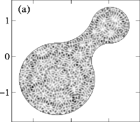
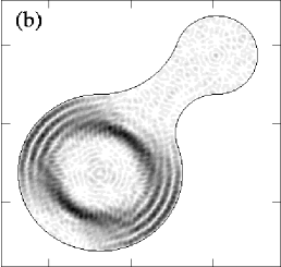
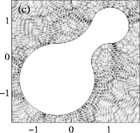
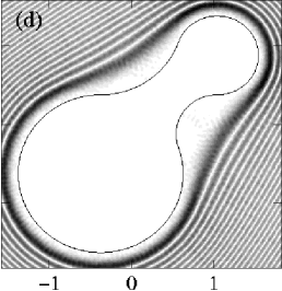
Figure 5.5: Interior and exterior wave functions of the skittle shape around the one-thousandth interior eigenstate, at fixed cyclotron radius $\rho=1.2$. The plotted shade is proportional to $|\psi|$ and the thin line indicates the boundary $\Gamma$. (a) A typical interior wave function, $\nu\simeq 32.9880$. (b) A bouncing ball mode, $\nu\simeq 33.1203$. (c) A typical exterior edge state, $\nu\simeq 32.8474$. (d) A typical exterior bulk state, $\nu\simeq 32.50025$. [figure quality reduced]

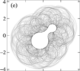
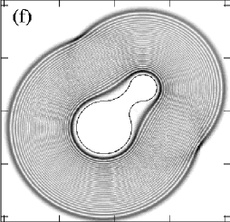
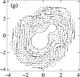
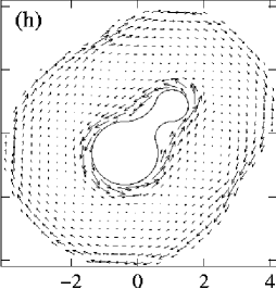
Figure 5.6: (continued) (e),(f) The same exterior edge and bulk states as in (c) and (d), respectively, on a larger scale. (g),(h) The current densities of the edge and bulk states (e) and (f), respectively. Here, the length of the arrows is proportional to the magnitude of the current density (measured at the at the tails of the arrows). [figure quality reduced]

Figure 5.5(a) shows the density plot of a typical interior wave function around the one-thousandth eigenstate. As expected for a classically chaotic system it spreads throughout the whole domain and has the features of a random wave. Occasionally, one also encounters so called bouncing-ball modes. These states are localized on a manifold of marginally stable periodic orbits (which have zero measure in phase space). In the skittle a prominent manifold consists of orbits with period 2 bouncing in the larger circular part of the billiard. The wave function of a corresponding bouncing-ball mode is given in Fig. 5.5(b).

We turn to the eigenstates of the exterior billiard. The wave function of a typical example may be found in Fig. 5.5(c). It belongs to an energy close to the one of Fig. 5.5(a) and is displayed on the same scale. Again, one observes the typical features of a chaotic wave function. When viewed on a larger scale, cf Fig. 5.5(e), we find that this state seems bound to the billiard and vanishes rapidly after a distance smaller than a cyclotron diameter. In addition, circular structures are faintly visible in the probability distribution with a radius given by the classical cyclotron radius $\rho=1.2$. This state is clearly an edge state corresponding classically to a skipping motion around the billiard. This is also evident from Fig. 5.5(g) which displays the distribution of the current density of the state.

Figure 5.5(d) shows a quite different exterior state. Its energy is still in the same range as that of Fig. 5.5(c) but now close to a Landau level. One observes that, unlike the edge state, the wave function shows no appreciable amplitude close to the boundary. Moreover, it displays a rather regular structure consisting of rings of maximal probability density which encircle the billiard. This is seen clearly on a larger scale, cf Fig. 5.5(f). The band running around the billiard has a width of the cyclotron diameter, $2\rho$, and in general consists of $N+1$ rings if the energy is close to $\nu=N+{\frac{1}{2}}$ (here $N=32$). This band moves outwards and gets more circular as one goes to bulk energies which are increasingly close to the Landau level (this way the bulk states in the sequence sweep over the whole plane). Clearly, we are dealing with a bulk state. Its wave function corresponds to a superposition of unperturbed cyclotron orbits which are placed around the billiard. This view is supported again by the distribution of the current density, cf Fig. 5.5(h). Near to the boundary it displays an opposite orientation compared to at a distance of $2\rho$. This renders the the net current around the billiard exponentially small — unlike the edge state Fig. 5.5(h) which displays a large finite current.

In order to see this separation into edge and bulk states more clearly we turn to even more semiclassical energies and a symmetric shape of the boundary.

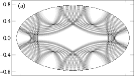
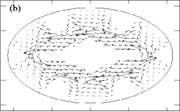
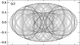
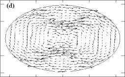
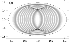
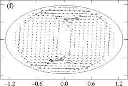
Figure 5.7: Probability densities (left) and current density distributions (right) in an elliptic domain at $\rho=0.6$, around the ten-thousandth interior eigenstate. (a,b) An edge state localized along a stable periodic orbit, $\nu\simeq 60.0602$. (c,d) A state which covers the whole domain $\nu\simeq 60.1664$. Note that the gross direction of the current changed compared to (b). (e,f) An interior bulk state, $\nu\simeq 60.50031$. The wave function is exponentially small close to the boundary and represents a superposition of cyclotron motion. [figure quality reduced]

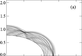
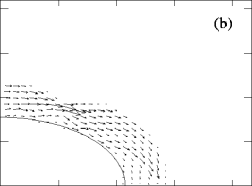
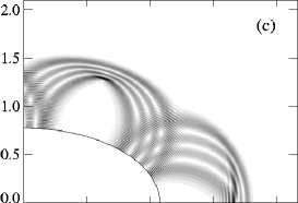
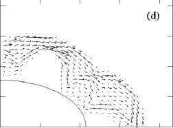
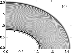
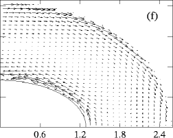
Figure 5.8: Exterior probability densities (left) and current density distributions (right) at $\rho=0.6$ and at similar energies as in Fig. 5.7. For each state only the first quarter of the picture is shown. (a,b) A typical edge state, $\nu\simeq 60.2087$. (c,d) An edge state localized along a stable periodic orbit, $\nu\simeq 60.2220$. (e,f) A typical bulk state, $\nu\simeq 60.50016$. [Possible Moire patterns in (e) are an effect of low resolution printing.] [figure quality reduced]

The ellipse

Next, we choose an elliptic boundary (of eccentricity $0.8$ and area $\pi$) and even more semiclassical energies. The cyclotron radius is taken to be $\rho=0.6$ which is small enough for complete cyclotron orbits to fit into the interior domain of the billiard. The classical dynamics of the skipping motion is mixed chaotic in this case [49], see Fig. 3.1 for a phase space portrait. Going to the extreme semiclassical limit – the ten-thousandth interior eigenstate – we expect the wave functions to mimic the structures of the underlying classical phase space. Indeed, Figure 5.7(a) displays a wave function which is localized along a stable interior periodic orbit. This orbit has period 36 traveling six times around the billiard, with six reflections each time, before it repeats itself. In contrast, the state in Fig. 5.7(c) is localized on a (mixed) chaotic part of phase space. We note that the gross circulation of the current density, Fig. 5.7(d), is opposite to that of the first state, Fig. 5.7(b). Since $\rho$ is small enough for closed cyclotron orbits to fit into the ellipse we find bulk states also in the interior, see Fig. 5.7(e) for an example. Again, it almost vanishes at the billiard boundary and may be viewed semiclassically as due to a superposition of closed cyclotron orbits. This view is supported by the distribution of the current density displayed in Fig. 5.7(f).

Similar states are also found in the exterior, as displayed in Figure 5.8. To show more details we give only the righthand-top quarter of the figure (the others follow by symmetry). The first edge state, Fig. 5.8(a), corresponds to a classical motion with creeps along the boundary. It is the analogue of a whispering-gallery mode. Figure 5.8(c) displays an exterior edge state which extends much further into the plane. Like Fig. 5.7(a) it is clearly localized on a stable skipping periodic orbit. The bulk state Fig. 5.8(e) is close to $\nu=60+{\frac{1}{2}}$. It consists of 61 concentric rings of increased amplitude and shows no appreciable net current around the billiard.

We emphasize that all the interior and exterior wave functions shown above are calculated throughout the entire displayed area. They turn out to be numerically zero in the complementary domains (ie, either the exterior or the interior) as expected from theory.

5.3 General boundary conditions

Figure 5.9: Contour plot of the ground state wave function (absolute value on a linear scale) for Neumann boundary conditions and strong field, $b=0.05$, $\nu\simeq 0.2763$. The wave function is localized at the boundary point of maximum curvature, as predicted by a recent theorem [110]. Here the billiard domain is given by the union of a half-circle and a half-ellipse (dashed line).

\psfrag{s}{$s$}\includegraphics[width=346.89731pt]{figs/helffergs_OnBoundaryLog.eps}

Figure 5.10: Boundary values of the ground state wave function of Fig. 5.9. As predicted in [110] it is localized exponentially at the point $s=0$ of maximum curvature.

The Neumann ground state

So far, we only considered Dirichlet boundary conditions. They are the natural choice from a physical point of view if one considers the billiard boundary as due to an infinite wall potential. On the other hand, the Neumann boundary conditions, $\Lambda^{-1}=0$, are frequently employed in spectral theory [22]. They have the advantage that the ground state energy lies below the first Landau level, which facilitates its mathematical analysis. Here, we are able to observe the manifestation of a recent theorem of spectral theory [110]. It states that the Neumann ground state of a magnetic billiard is exponentially localized around the boundary point of maximum curvature. In order to deal with a unique boundary point of maximum curvature we choose the union of a half-circle and a half-ellipse (with half-axes $\check{a}=2,\check{b}=0.5$) as billiard boundary. Choosing a magnetic length of $b=0.05$ (which corresponds to a very strong field), we find the ground state energy $\nu=0.2763$. The Figures 5.9 and 5.10 display the ground state wave function in the billiard and on the boundary, respectively. Indeed, one observes an exponential localization over six orders of magnitude.

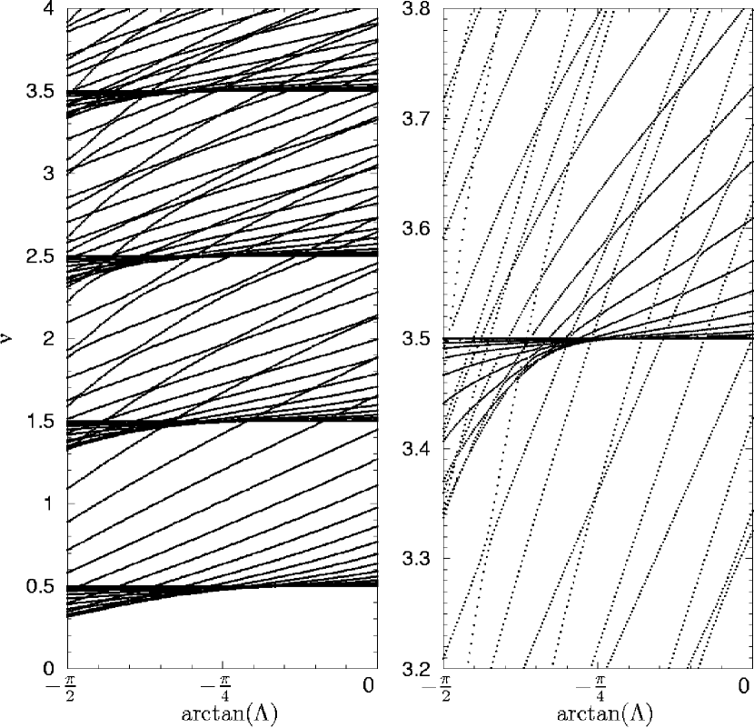
Figure 5.11: The parametric dependence of the exterior spectrum on the boundary condition (for the asymmetric stadium, ie $\mathrsfs{L}=5.39724$, at fixed $b=0.25$). The parameter $\Lambda$ interpolates between Neumann ($\arctan\Lambda=-\frac{\pi}{2}$) and Dirichlet ($\arctan\Lambda=0$) boundary conditions. The right graph shows details around the fourth Landau level. [figure quality reduced]

Parametric dependence on the mixing parameter

As a last point, we show the parametric dependence of a spectrum on the type of boundary conditions. Figure 5.11 presents the exterior spectrum of the asymmetric stadium as a function of the scaled mixing parameter $\Lambda\in(-\infty,0]$, cf (3.7). It is chosen negative to ensure that the transformation from Neumann ($\Lambda=-\infty$) to Dirichlet ($\Lambda=0$) boundary conditions is continuous. For positive $\Lambda$ this would not be the case, which is a restriction similar to the one for the field free case [76]. ( We use the the $\arctan$ function in Fig. 5.11 to transform the infinite range of $\Lambda$ into a bounded interval.)

One observes that all the energy levels increase monotonically as $\Lambda$ is increased. The energies clustering around the Landau levels $\nu=N+\tfrac{1}{2},N\in{{{\mathbb{N}}}_{0}}$ belong to bulk states. One observes that they are lifted from the Landau levels to higher energies at Dirichlet boundary conditions, whereas in the Neumann case they are always shifted to smaller energies. A semiclassical theory which describes the exponential approach of the bulk states to the Landau levels and their behavior as a function of $\Lambda$ is given in Appendix A.6.3 and Section 7.3.1. We shall come back to Fig. 5.11 not only there, but also in Chapter 7, when we define the edge state density.

6 Semiclassical Quantization

In Chapter 4 the boundary integral equations were found to yield an efficient method for obtaining the exact quantum spectrum of magnetic billiards. It will be shown in the sequel that the same equations are as important for the semiclassical quantization: They serve as the starting point for the derivation of the semiclassical trace formulas.

Periodic orbit formulas for magnetic billiards

The celebrated trace formulas of Gutzwiller [111, 27] and Berry & Tabor [112, 113] allow the semiclassical quantization of systems in terms of their classical motion. They were derived assuming a continuous Hamiltonian flow. The corresponding formulas for field free billiards are known to exhibit additional phase factors which account for the billiard boundary conditions. In order to show that the same holds for magnetic billiards we shall explain how the corresponding trace formulas are obtained from the exact boundary integral formalism. To our knowledge no such derivation has been published for magnetic billiards to date. The natural approach is to follow the lines of Balian and Bloch’s treatment of field-free billiards [114, 115], in analogy to the surface-of-section method [116] and the scattering approach [117] for non-magnetic systems. Those attempts failed so far for magnetic billiards due to the appearance of an abundance of unphysical “ghost” orbits which could not be handled. To resolve this problem we take advantage of the analysis performed in Chapter 4. There it was found that the boundary integral equations include spurious solutions which belong to a particular complementary problem. We will show that the semiclassical spectral determinant can be factorized, accordingly, into an interior and exterior part. Each of them leads to a trace formula incorporating only the physical periodic orbits in the appropriate domain.

Like in the field-free case [114, 115, 116, 117, 118, 119, 120] the semiclassical quantization will be based on the double layer boundary integral equation. Apart from the spurious solutions, the main complication arising at finite magnetic field is the inherently asymmetric form of the respective integral kernel. Unlike the case of field-free billiards [60], the latter is not simply related to the semiclassically unitary map operator derived from the generating function.

In Section 6.1 we deduce the semiclassical approximants to the boundary integral operators of Chapter 4. After that, in Sect. 6.2, special map operators are introduced in order to transform the spectral function of the double-layer boundary integral equation. As a result, the number counting function is given in terms of the traces of powers of the map operators. The traces are evaluated semiclassically in Section 6.3 assuming hyperbolic skipping motion. We show why only classically allowed periodic orbits contribute and how their stability properties enter. The section concludes with the trace formula for the density of states and the magnetization density. In Section 6.4 the traces are evaluated assuming integrable dynamics. As a result we obtain the explicit periodic orbit formula for the spectral density of states in the magnetic disk billiard. Section  6.5 gives the corresponding WKB solution.

6.1 The semiclassical boundary integral operators

In Section 4.3 the boundary integral operators were defined in terms of the free Green function and derivatives thereof. To obtain the semiclassical approximations of the operators one simply replaces the Green function by its approximant. The latter is the leading order asymptotic expression in the semiclassically small parameter $\nu^{-1}$, which was derived in Sect. 2.5.1. To remain at a consistent level of approximation, the derivatives appearing in the single-layer Neumann and the double-layer operators (4.11) – (4.13) are to be evaluated to the same leading order. This means in practice, that only the phase of the Green function (2.58) must be differentiated. Accordingly, in the remainder of this report all equalities involving semiclassical quantities are understood to be semiclassical in the sense that they hold to leading order in $\nu^{-1}$.

In order to obtain expressions which have a semiclassically intuitive and useful form it will be important to use the representation (2.58) which contains the actions of the short and long arcs separately. We found the geometric parts of the corresponding scaled actions (2.5.1) to be given by

$${\rm a}_{\rm S}(\mathbf{r};\mathbf{r}_{0}) =\frac{1}{\pi}\bigg{(}\arcsin\left(\frac{|\mathbf{r}-\mathbf{r}_{0}|}{2\rho}\right)+\frac{|\mathbf{r}-\mathbf{r}_{0}|}{2\rho}\sqrt{1-\left(\frac{\mathbf{r}-\mathbf{r}_{0}}{2\rho}\right)^{2}}-\frac{\mathbf{r}\times\mathbf{r}_{0}}{2\rho^{2}}\bigg{)}$$ (6.1)

and

$${\rm a}_{\rm L}(\mathbf{r};\mathbf{r}_{0}) =1-{\rm a}_{\rm S}(\mathbf{r}_{0};\mathbf{r})\ .$$ (6.2)

As a first step, we note their gradients with respect to the initial and the final points.

$${\boldsymbol{\nabla}}_{\!\mathbf{r}_{0}}\,{\rm a}_{\left(\begin{smallmatrix}{\rm S}\\ {\rm L}\end{smallmatrix}\right)}(\mathbf{r};\mathbf{r}_{0}) =\frac{1}{\pi\rho}\left(\mp\frac{\mathbf{r}-\mathbf{r}_{0}}{|\mathbf{r}-\mathbf{r}_{0}|}\sqrt{1-\left(\frac{\mathbf{r}-\mathbf{r}_{0}}{2\rho}\right)^{2}}-\frac{1}{2\rho}{-y\choose x}\right)$$ (6.3)

$${\boldsymbol{\nabla}}_{\!\mathbf{r}}\,{\rm a}_{\left(\begin{smallmatrix}{\rm S}\\ {\rm L}\end{smallmatrix}\right)}(\mathbf{r};\mathbf{r}_{0}) =\frac{1}{\pi\rho}\left(\pm\frac{\mathbf{r}-\mathbf{r}_{0}}{|\mathbf{r}-\mathbf{r}_{0}|}\sqrt{1-\left(\frac{\mathbf{r}-\mathbf{r}_{0}}{2\rho}\right)^{2}}+\frac{1}{2\rho}{-y_{0}\choose x_{0}}\right)$$ (6.4)

Here, the upper and lower signs of the first summands stand for the short arc and long arc contribution, respectively. It will be useful to state the distance between the initial and the final point in terms of the positive angle

$$\alpha(\mathbf{r};\mathbf{r}_{0}):=\arcsin\left(\frac{|\mathbf{r}-\mathbf{r}_{0}|}{2\rho}\right)\ .$$ (6.5)

In addition, the direction of the normal vectors at the initial and the final points are measured by their (signed) angles with respect to the distance vector connecting the two points.

$$\beta(\mathbf{r};\mathbf{r}_{0}):=\raisebox{-0.6458pt}{\Large$\sphericalangle$}(\hat{\mathbf{n}};\mathbf{r}-\mathbf{r}_{0})\qquad\beta^{0}(\mathbf{r};\mathbf{r}_{0}):=\raisebox{-0.6458pt}{\Large$\sphericalangle$}(\hat{\mathbf{n}}_{0};\mathbf{r}-\mathbf{r}_{0})$$ (6.6)

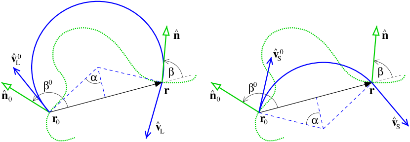
Figure 6.1: The angles $\alpha$, $\beta^{0}$, and $\beta$ are defined with respect the vector $\mathbf{r}-\mathbf{r}_{0}$ connecting the initial and the final point. They measure its length and the relative direction of the boundary normals, respectively. These quantities do not depend on the type of the arc (left: long, right: short), unlike the relative direction of the initial and the final velocities $\hat{\mathbf{v}}^{0}$ and $\hat{\mathbf{v}}$. The latter may be expressed in terms of $\alpha$, $\beta^{0}$, and $\beta$, cf (6.1). (The dotted line indicates the billiard boundary.)

Now consider the classical arcs connecting the initial and the final points. They define the direction of the classical velocities at the points of reflection and incidence (see Figure 6.1 for a sketch of the situation). The normal components are given by

$$\hat{\mathbf{v}}_{\rm S}\,\hat{\mathbf{n}} =\cos(\beta+\alpha) \qquad\hat{\mathbf{v}}^{0}_{\rm S}\,\hat{\mathbf{n}}_{0} =\cos(\beta^{0}-\alpha)$$

$$\hat{\mathbf{v}}_{\rm L}\,\hat{\mathbf{n}} =-\cos(\beta-\alpha) \qquad\hat{\mathbf{v}}^{0}_{\rm L}\,\hat{\mathbf{n}}_{0} =-\cos(\beta^{0}+\alpha)$$ (6.7)

for short and long arcs, respectively. Here, the velocity at the initial point of the arc is denoted with a zero superscript, and the hats indicate that the velocity vectors are normalized.

The semiclassical Dirichlet operators

We proceed to calculate the semiclassical approximation to the kernel of the double layer Dirichlet operator (4.12) by inserting (2.58). For the short arc term one has to evaluate the gauge invariant derivative

$$\partial_{n_{0}/b}[2\pi\mathrm{i}\nu{\rm a}_{\rm S}-\tilde{\chi}_{0}]+\mathrm{i}\tilde{A}_{n_{0}} =2\mathrm{i}\sqrt{\nu}\left(-\frac{(\mathbf{r}-\mathbf{r}_{0})\,\hat{\mathbf{n}}_{0}}{|\mathbf{r}-\mathbf{r}_{0}|}\cos(\alpha)-\frac{(\mathbf{r}-\mathbf{r}_{0})\times\hat{\mathbf{n}}_{0}}{2\rho}\right)$$

$$=-2\mathrm{i}\sqrt{\nu}\,\cos(\beta^{0}-\alpha)=-2\mathrm{i}\sqrt{\nu}\,(\hat{\mathbf{v}}^{0}_{\rm S}\,\hat{\mathbf{n}}_{0})\ ,$$ (6.8)

where we used eqs (6.3) and (6.1). Apart from the sign, it is given by the normal component of the classical velocity after reflection since $2\sqrt{\nu}$ is the magnitude of the scaled velocity. Note that $(\hat{\mathbf{v}}^{0}_{\rm S}\,\hat{\mathbf{n}}_{0})$ is a non-symmetric function of the initial and the final point and depends on the energy through $\alpha$. For the long arc term one obtains the analogous expression

$$\partial_{n_{0}/b}[2\pi\mathrm{i}\nu{\rm a}_{\rm L}-\tilde{\chi}_{0}]+\mathrm{i}\tilde{A}_{n_{0}} =+2\mathrm{i}\sqrt{\nu}\,\cos(\beta^{0}+\alpha)=-2\mathrm{i}\sqrt{\nu}\,(\hat{\mathbf{v}}^{0}_{\rm L}\,\hat{\mathbf{n}}_{0})\ .$$ (6.9)

It follows that the semiclassical approximation of the double-layer Dirichlet kernel (4.27) can be stated in a particularly simple form,

$${\rm q}^{\rm D(sc)}_{\rm dl}(\mathbf{r};\mathbf{r}_{0}):=\partial_{n_{0}/b}{\rm G}^{\rm(sc)}_{\nu}+\mathrm{i}\tilde{A}_{n_{0}}{\rm G}^{\rm(sc)}_{\nu}=\frac{1}{2(1+\mathrm{e}^{2\pi\mathrm{i}\nu})}\,\frac{1}{(2\pi\mathrm{i})^{\frac{1}{2}}}\,\mathrm{e}^{\mathrm{i}(\tilde{\chi}-\tilde{\chi}_{0})}\\ \times\left\{\frac{-\hat{\mathbf{v}}^{0}_{\rm S}\,\hat{\mathbf{n}}_{0}}{(\sin\alpha\cos\alpha)^{\frac{1}{2}}}\,\mathrm{e}^{2\pi\mathrm{i}\nu{\rm a}_{\rm S}}+\mathrm{e}^{-\mathrm{i}\frac{\pi}{2}}\,\frac{-\hat{\mathbf{v}}^{0}_{\rm L}\,\hat{\mathbf{n}}_{0}}{(\sin\alpha\cos\alpha)^{\frac{1}{2}}}\,\mathrm{e}^{2\pi\mathrm{i}\nu{\rm a}_{\rm L}}\right\}\ .$$ (6.10)

It will be an important ingredient in the derivation of the trace formulas.For completeness we note that the semiclassical single-layer Dirichlet kernel is simply given by the semiclassical Green function itself, ${\rm q}^{\rm D(sc)}_{\rm sl}(\mathbf{r};\mathbf{r}_{0}):={\rm G}^{\rm(sc)}_{\nu}$, as an immediate consequence of (4.10).

The semiclassical Neumann operators

The kernels of the single- and double layer Neumann operators, eqs (4.11) and (4.13), involve gauge invariant gradients with respect to the final point of the Green function. One finds

$$\partial_{n/b}[2\pi\mathrm{i}\nu{\rm a}_{\rm S}+\tilde{\chi}]-\mathrm{i}\tilde{A}_{n} =+2\mathrm{i}\sqrt{\nu}\,\cos(\beta+\alpha)=+2\mathrm{i}\sqrt{\nu}\,(\hat{\mathbf{v}}_{\rm S}\,\hat{\mathbf{n}})\ ,$$ (6.11)

$$\partial_{n/b}[2\pi\mathrm{i}\nu{\rm a}_{\rm L}+\tilde{\chi}]-\mathrm{i}\tilde{A}_{n} =-2\mathrm{i}\sqrt{\nu}\,\cos(\beta-\alpha)=+2\mathrm{i}\sqrt{\nu}\,(\hat{\mathbf{v}}_{\rm L}\,\hat{\mathbf{n}})\ ,$$ (6.12)

similar to eqs (6.1) and (6.9). This way the semiclassical single-layer Neumann kernel (4.26) assumes the form

$${\rm q}^{\rm N(sc)}_{\rm sl}(\mathbf{r};\mathbf{r}_{0}):=\partial_{n/b}{\rm G}^{\rm(sc)}_{\nu}-\mathrm{i}\tilde{A}_{n}{\rm G}^{\rm(sc)}_{\nu}=\frac{1}{2(1+\mathrm{e}^{2\pi\mathrm{i}\nu})}\,\frac{1}{(2\pi\mathrm{i})^{\frac{1}{2}}}\,\mathrm{e}^{\mathrm{i}(\tilde{\chi}-\tilde{\chi}_{0})}\\ \times\left\{\frac{+\hat{\mathbf{v}}_{\rm S}\,\hat{\mathbf{n}}}{(\sin\alpha\cos\alpha)^{\frac{1}{2}}}\,\mathrm{e}^{2\pi\mathrm{i}\nu{\rm a}_{\rm S}}+\mathrm{e}^{-\mathrm{i}\frac{\pi}{2}}\,\frac{+\hat{\mathbf{v}}_{\rm L}\,\hat{\mathbf{n}}}{(\sin\alpha\cos\alpha)^{\frac{1}{2}}}\,\mathrm{e}^{2\pi\mathrm{i}\nu{\rm a}_{\rm L}}\right\}$$ (6.13)

It is worth noting how the mutual adjointness of the operators (4.26) and (4.27) shows up in the semiclassical case. By permuting $\mathbf{r}$ and $\mathbf{r}_{0}$ the prefactors of the short and long arc terms change their roles,

$$(\hat{\mathbf{v}}_{\rm S}\,\hat{\mathbf{n}})\equiv\hat{\mathbf{v}}_{\rm S}(\mathbf{r};\mathbf{r}_{0})\,\hat{\mathbf{n}}(\mathbf{r})=\hat{\mathbf{v}}^{0}_{\rm L}(\mathbf{r}_{0};\mathbf{r})\,\hat{\mathbf{n}}(\mathbf{r}_{0})\equiv(\hat{\mathbf{v}}^{0}_{\rm L}\,\hat{\mathbf{n}}_{0})^{\dagger}\ ,$$ (6.14)

and likewise $(\hat{\mathbf{v}}_{\rm L}\,\hat{\mathbf{n}})=(\hat{\mathbf{v}}^{0}_{\rm S}\,\hat{\mathbf{n}}_{0})^{\dagger}$. As for the phases, it is the factor $(1+\mathrm{e}^{2\pi\mathrm{i}\nu})^{-1}$ whose conjugation provides the term $\mathrm{e}^{2\pi\mathrm{i}\nu}$ needed in conjunction with the relation (6.2) to prove the mutual adjointness.

The kernel of the semiclassical double-layer Neumann operator follows from applying the gauge invariant derivative (6.11) to the single-layer Dirichlet expression (6.10), cf (4.13). One obtains

$$\begin{aligned} \,&{\rm q}^{\rm N(sc)}_{\rm dl}(\mathbf{r};\mathbf{r}_{0}):=\,(\partial_{n_{0}/b}+\mathrm{i}\tilde{A}_{n_{0}})(\partial_{n/b}{\rm G}^{\rm(sc)}_{\nu}-\mathrm{i}\tilde{A}_{n}{\rm G}^{\rm(sc)}_{\nu})\,\\ \,&=\,\frac{1}{2(1+\mathrm{e}^{2\pi\mathrm{i}\nu})}\,\frac{2\mathrm{i}\sqrt{\nu}}{(2\pi\mathrm{i})^{\frac{1}{2}}}\,\mathrm{e}^{\mathrm{i}(\tilde{\chi}-\tilde{\chi}_{0})}\end{aligned}\\ \times\left\{\frac{-(\hat{\mathbf{v}}^{0}_{\rm S}\,\hat{\mathbf{n}}_{0})(\hat{\mathbf{v}}_{\rm S}\,\hat{\mathbf{n}})}{(\sin\alpha\cos\alpha)^{\frac{1}{2}}}\,\mathrm{e}^{2\pi\mathrm{i}\nu{\rm a}_{\rm S}}+\mathrm{e}^{-\mathrm{i}\frac{\pi}{2}}\,\frac{-(\hat{\mathbf{v}}^{0}_{\rm L}\,\hat{\mathbf{n}}_{0})(\hat{\mathbf{v}}_{\rm L}\,\hat{\mathbf{n}})}{(\sin\alpha\cos\alpha)^{\frac{1}{2}}}\,\mathrm{e}^{2\pi\mathrm{i}\nu{\rm a}_{\rm L}}\right\}\ .$$ (6.15)

Like the exact kernel (4.3) this semiclassical version is self-adjoint. This follows again from the observation that the two summands simply change roles when the adjoint operator is formed.

6.2 From boundary to map operators

Let us now consider the semiclassical double-layer equation for Dirichlet boundary conditions in more detail. As known from Chapter 4 the corresponding Fredholm determinant (4.15) is a spectral function. Its roots yield the Dirichlet spectrum of the domain considered, conjoint with the Neumann spectrum of the complementary domain.

The semiclassical spectral function is obtained by substituting (6.10) into (4.15) with $\lambda=0$:

$$\xi^{\rm(sc)}(\nu):= \det\left[{\frac{1}{2}}\pm{\sf Q}_{\rm dl}^{\rm D(sc)}\right]$$ (6.16)

Here, the upper or lower sign indicates whether the originally considered domain is of the interior or the exterior type (like in Chapter 4).

The map operators

By defining the operator

$${\sf P}:=2(1+\mathrm{e}^{2\pi\mathrm{i}\nu})\,{\sf Q^{\rm D\,(sc)}_{\rm dl}}\ .$$ (6.17)

we factorize the determinant 6.16 into two parts,

$$\xi^{\rm(sc)}(\nu)=\det\left[\frac{1}{2(1+\mathrm{e}^{2\pi\mathrm{i}\nu})}\right]\,\det\left[1+\mathrm{e}^{2\pi\mathrm{i}\nu}\pm{\sf P}\right]\ .$$ (6.18)

This reflects the partitioning of the underlying classical phase space into cyclotron orbits, which are detached from the boundary, and skipping trajectories, see Sect. 3.1. The first determinant in (6.18) does not depend on the boundary. Its operator is diagonal and singular at the energies $\nu_{N}=N+{\frac{1}{2}}$, $N\in{{{\mathbb{N}}}_{0}}$, of the Landau levels. Apparently, it represents the semiclassical contribution of the bulk states to the spectrum and its divergence at the Landau energies is due to the infinite number of degenerate bulk states found in the exterior. (The exponentially small lifting of the degeneracy observed in the exact spectrum is not seen here since the semiclassical Green function (2.59) does not describe tunneling effects.)

As will become clear in the following, the second factor in (6.18) yields the contribution of the skipping trajectories to the spectral function. It is described by the map operator ${\sf P}$ defined in (6.17). We will see that it can be related to the classical billiard map (3.4) describing the motion of skipping trajectories. The map operator consists of a short arc and a long arc term and it is advantageous to split it accordingly,

$${\sf P}={\sf P}_{\rm S}+{\sf P}_{\rm L}\ ,$$ (6.19)

with the corresponding integral kernels given by

$${\rm p}_{\rm S}(s,s_{0}) :=\frac{1}{(2\pi\mathrm{i})^{\frac{1}{2}}}\,\frac{-\hat{\mathbf{v}}^{0}_{\rm S}\,\hat{\mathbf{n}}_{0}}{(\sin(\alpha)\cos(\alpha))^{\frac{1}{2}}}\,\,\mathrm{e}^{2\pi\mathrm{i}\nu{\rm a}_{\rm S}}\,\mathrm{e}^{\mathrm{i}\tilde{\chi}-\mathrm{i}\tilde{\chi}_{0}}$$ (6.20)

and

$${\rm p}_{\rm L}(s,s_{0}) :=\frac{1}{(2\pi\mathrm{i})^{\frac{1}{2}}}\,\frac{-\hat{\mathbf{v}}^{0}_{\rm L}\,\hat{\mathbf{n}}_{0}}{(\sin(\alpha)\cos(\alpha))^{\frac{1}{2}}}\,\,\mathrm{e}^{-\mathrm{i}\frac{\pi}{2}}\,\mathrm{e}^{2\pi\mathrm{i}\nu{\rm a}_{\rm L}}\,\mathrm{e}^{\mathrm{i}\tilde{\chi}-\mathrm{i}\tilde{\chi}_{0}}\ ,$$ (6.21)

see (6.10), with $\mathbf{r}=\mathbf{r}(s),\mathbf{r}_{0}=\mathbf{r}(s_{0})$.

We note that the operator P differs from the standard map operator defined in terms of the generating function $\mathrsfs{G}$ of the classical map [60],

$${\sf S}=-\frac{1}{(2\pi\mathrm{i})^{\frac{1}{2}}}\left(\frac{\partial^{2}\mathrsfs{G}}{\partial s\partial s_{0}}\right)^{\frac{1}{2}}\mathrm{e}^{\mathrm{i}\mathrsfs{G}}\ ,$$ (6.22)

which is the analogue of Bogomolny’s transfer operator ${\sf T}$ [116]. The main difference is not the fact that ${\sf P}$ consists of two distinct parts. Rather, it is the inherent asymmetry in the coordinates $s,s_{0}$ which introduces difficulties not encountered in the field-free treatment: The prefactors cannot in general be stated as mixed derivatives of the relevant phase. Moreover, the parts ${\sf P}_{\rm\!S/L}$ are not semiclassically unitary (but satisfy equation (6.25)).

From now on we focus on the non-singular factor in (6.16). It gives the spectral function

$$\xi^{\rm(sc)}_{\rm skip}(\nu)= \det\left[1+\mathrm{e}^{2\pi\mathrm{i}\nu}\pm{\sf P}\right]$$ (6.23)

of the states which correspond to skipping motion. In the standard procedure to obtain a trace formula one would now compute the imaginary part of the logarithm of (6.23). Making use of the identity $\log\det=\mathop{\mathrm{tr}}\nolimits\log$ [121] one would like to evaluate the trace of powers of the operator (6.19) in stationary phase approximation. However, unlike the case of field-free billiards the corresponding saddle point condition selects classical periodic orbits in the interior and in the exterior. This is not surprising given the fact that the double-layer equation includes solutions of the complementary domain. To make matters worse, an abundance of saddle-point configurations arises which do not have a physical meaning at all. In order to avoid these severe difficulties it is vital to write the spectral function (6.23) as a product such that each factor yields the spectrum in either the interior or the exterior domain.

Factorizing the spectral function

To facilitate the factorization of the determinant (6.23) we split the short and long arc operators once more, ${\sf P}_{\rm S}={\sf P}_{\rm S}^{\rm int}-{\sf P}_{\rm S}^{\rm ext}$ and ${\sf P}_{\rm L}={\sf P}_{\rm L}^{\rm int}-{\sf P}_{\rm L}^{\rm ext}$. Ultimately, the parts labeled by “int”and “ext” should exclusively account for the motion in the interior and in the exterior, respectively. To that end, the splitting is defined by the signs of the prefactors of the integral kernels which are functions of the initial and the final points.

$${\rm p}_{\rm S}^{\rm int}(s,s_{0}) :=\Theta(-\hat{\mathbf{n}}_{0}\hat{\mathbf{v}}^{0}_{\rm S})\,{\rm p}_{\rm S}(s,s_{0}) \qquad{\rm p}_{\rm L}^{\rm int}(s,s_{0}) :=\Theta(-\hat{\mathbf{n}}_{0}\hat{\mathbf{v}}^{0}_{\rm L})\,{\rm p}_{\rm L}(s,s_{0})$$

$${\rm p}_{\rm S}^{\rm ext}(s,s_{0}) :=-\Theta(\hat{\mathbf{n}}_{0}\hat{\mathbf{v}}^{0}_{\rm S})\,{\rm p}_{\rm S}(s,s_{0}) \qquad{\rm p}_{\rm L}^{\rm ext}(s,s_{0}) :=-\Theta(\hat{\mathbf{n}}_{0}\hat{\mathbf{v}}^{0}_{\rm L})\,{\rm p}_{\rm L}(s,s_{0})$$

(The minus sign in front of the exterior kernels is introduced for convenience.) According to these definitions the “interior” part of the operators vanishes whenever the initial and the final points have positions such that the corresponding classical arc points into the exterior domain, and vice versa. This crucial property is embodied in the operator equations

$${\sf P}_{\rm S}^{\rm int}\,{\sf P}_{\rm L}^{\rm ext}+{\sf P}_{\rm L}^{\rm int}\,{\sf P}_{\rm S}^{\rm ext} =-\,\mathrm{e}^{2\pi\mathrm{i}\nu}\,{\sf id}$$ (6.25)

and

$${\sf P}_{\rm S}^{\rm int}\,{\sf P}_{\rm S}^{\rm ext}+{\sf P}_{\rm L}^{\rm int}\,{\sf P}_{\rm L}^{\rm ext} =0\ ,$$ (6.26)

derived in Appendix A.5. With their help it follows immediately that the determinant in eq (6.23) factorizes into an interior and an exterior part,

$$\xi^{\rm(sc)}_{\rm skip}(\nu) =\det\left[1+\mathrm{e}^{2\pi\mathrm{i}\nu}\pm\big{(}{\sf P}_{\rm S}^{\rm int}-{\sf P}_{\rm S}^{\rm ext}+{\sf P}_{\rm L}^{\rm int}-{\sf P}_{\rm L}^{\rm ext}\big{)}\right]$$

$$=\det\left[\Big{(}1\pm\big{(}{\sf P}_{\rm S}^{\rm int}+{\sf P}_{\rm L}^{\rm int}\big{)}\Big{)}\Big{(}1\mp\big{(}{\sf P}_{\rm S}^{\rm ext}+{\sf P}_{\rm L}^{\rm ext}\big{)}\Big{)}\right]$$

$$=\det\left[1\pm{\sf P}^{\rm int}\right]\,\det\left[1\mp{\sf P}^{\rm ext}\right]\ .$$ (6.27)

Here we merely replaced the term $\mathrm{e}^{2\pi\mathrm{i}\nu}$ by the operators (6.25) and included (6.26). In the last equality we introduced the interior and exterior map operators ${\sf P}^{\rm int}:={\sf P}_{\rm S}^{\rm int}+{\sf P}_{\rm L}^{\rm int}$ and ${\sf P}^{\rm ext}:={\sf P}_{\rm S}^{\rm ext}+{\sf P}_{\rm L}^{\rm ext}$, respectively.

The factorization of the spectral function (6.2) into an interior and exterior part is in accordance with the observation that the double layer equation provides the spectra of both the interior and the exterior problems, see the discussion in Sect. 4.2.2. In the following section we shall show that using the upper sign, ie, starting originally with the interior problem, one gets the trace formula for the interior Dirichlet spectrum from the first factor and the exterior Neumann spectrum from the second one. In the same way, if we use the lower sign we get the trace formula for the exterior Dirichlet spectrum from the second factor and the interior Neumann spectrum from the first.

We finally note that the operators ${\sf P}^{\rm int}$ and ${\sf P}^{\rm ext}$ are semiclassically unitary, as shown in Appendix A.5. Moreover, the interior and exterior map operators obey the relation

$${\sf P}^{\rm int}{\sf P}^{\rm ext}=-\mathrm{e}^{2\pi\mathrm{i}\nu}{\sf id}\ ,$$ (6.28)

which follows from (6.25) and (6.26). It has an intuitive form: Propagating a boundary state first in the exterior and then in the interior one arrives again at the same state, augmented by the global phase $2\pi\nu$ of a complete cyclotron orbit (plus the Maslov correction $\pi$). It is the semiclassical manifestation of the classical interior-exterior duality.

6.3 Trace formula for hyperbolic billiards

To obtain the fluctuating part of the number counting function of the skipping spectrum one has to take the imaginary part of the logarithm of the spectral function (6.2). We start by computing the contribution of the first factor in (6.2),

$${\rm N}^{\rm skip(int)}_{\rm osc}(\nu)= -\frac{1}{\pi}\mathop{\mathrm{Im}}\nolimits\log\det\left[1\pm{\sf P}^{\rm int}\right]=\frac{1}{\pi}\mathop{\mathrm{Im}}\nolimits\sum_{n=1}^{\infty}\frac{(\mp)^{n}}{n}\,\mathop{\mathrm{tr}}\nolimits\!\left[\big{(}{\sf P}^{\rm int}\big{)}^{n}\right]$$ (6.29)

To obtain the periodic orbit formula we can now follow the lines of the derivation of the trace formula for field free billiards [114, 116, 115, 99, 118, 119, 122, 123, 120]. The trace in (6.29) amounts to an $n$-dimensional integral of the form

$$\mathop{\mathrm{tr}}\nolimits\!\left[\big{(}{\sf P}^{\rm int}\big{)}^{n}\right]=\frac{1}{(2\pi\mathrm{i})^{n/2}}\int\frac{\mathrm{d}s_{1}\ldots\mathrm{d}s_{n}}{b^{n}}\,\exp\Big{(}{\mathrm{i}\sum_{j=1}^{n}(\widetilde{{\raisebox{0.43057pt}{\large$\chi$}}}(s_{j+1})-\widetilde{{\raisebox{0.43057pt}{\large$\chi$}}}(s_{j}))}\Big{)}$$

$$\begin{aligned} \times\prod_{j=1}^{n}\Bigg{[}&\frac{-(\hat{\mathbf{v}}^{0}_{\rm S}\hat{\mathbf{n}}_{0})_{j}\,\Theta\big{(}-(\hat{\mathbf{v}}^{0}_{\rm S}\hat{\mathbf{n}}_{0})_{j}\big{)}}{\big{(}\sin(\alpha_{j})\cos(\alpha_{j})\big{)}^{\frac{1}{2}}}\exp\Big{(}{2\pi\mathrm{i}\nu{\rm a}_{\rm S}(s_{j+1};s_{j})}\Big{)}\\ &+\frac{-(\hat{\mathbf{v}}^{0}_{\rm L}\hat{\mathbf{n}}_{0})_{j}\,\Theta\big{(}-(\hat{\mathbf{v}}^{0}_{\rm L}\hat{\mathbf{n}}_{0})_{j}\big{)}}{\big{(}\sin(\alpha_{j})\cos(\alpha_{j})\big{)}^{\frac{1}{2}}}\exp\Big{(}{2\pi\mathrm{i}\nu{\rm a}_{\rm L}(s_{j+1};s_{j})-\mathrm{i}\frac{\pi}{2}}\Big{)}\Bigg{]}\ .\end{aligned}$$

Here, the abbreviation $(\hat{\mathbf{v}}^{0}\hat{\mathbf{n}}_{0})_{j}:=\hat{\mathbf{v}}^{0}(\mathbf{r}(s_{j+1});\mathbf{r}(s_{j}))\,\hat{\mathbf{n}}(\mathbf{r}(s_{j}))$ is used, together with (6.32) and the convention $s_{0}\equiv s_{n}$. Note that the gauge dependent factor (involving the $\widetilde{{\raisebox{0.43057pt}{\large$\chi$}}}(s_{j})$) vanishes identically as a consequence of the cyclic permutability of the integration variables. This renders the trace (6.3) a gauge invariant quantity. It is now evaluated to leading semiclassical order using the stationary phase approximation (A.30).

6.3.1 The saddle point conditions

For each of the $2^{n}$ integrands in (6.3) the condition of a stationary phase leads to $n$ saddle point equations

$$\frac{\mathrm{d}}{\mathrm{d}s_{j}}\Big{[}2\pi\nu{\rm a}_{\eta_{j}}(s_{j};s_{j-1})+2\pi\nu{\rm a}_{\eta_{j+1}}(s_{j+1};s_{j})\Big{]}\stackrel{{\scriptstyle!}}{{=}}0\ ,\quad j\in\{1,\ldots,n\}\ .$$ (6.31)

Here, the indices $\eta_{j}\in\{{\rm S},{\rm L}\}$ account for the $2^{n}$ different sequences of short and long arc operators under the trace. We shall treat all these equations simultaneously by noting for any solution $\underline{s}$ of (6.31) not only the configuration of saddle points but also the corresponding sequence of types of arcs, $\underline{s}=((s_{1},\eta_{1}),..,(s_{n},\eta_{n}))$.

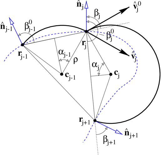
Figure 6.2: The angles entering the $j$th saddle point condition. (The dashed line indicates the boundary.)

$\displaystyle\hat{\mathbf{n}}_{j}\,\hat{\mathbf{v}}^{0}_{{\rm S}\,j}$ $\displaystyle=+\cos(\beta^{0}_{j}-\alpha_{j})$ $\displaystyle\qquad\hat{\mathbf{t}}_{j}\,\hat{\mathbf{v}}^{0}_{{\rm S}\,j}$ $\displaystyle=-\sin(\beta^{0}_{j}-\alpha_{j})$ $\displaystyle\hat{\mathbf{n}}_{j}\,\hat{\mathbf{v}}^{0}_{{\rm L}\,j}$ $\displaystyle=-\cos(\beta^{0}_{j}+\alpha_{j})$ $\displaystyle\qquad\hat{\mathbf{t}}_{j}\,\hat{\mathbf{v}}^{0}_{{\rm L}\,j}$ $\displaystyle=+\sin(\beta^{0}_{j}+\alpha_{j})$ $\displaystyle\hat{\mathbf{n}}_{j}\,\hat{\mathbf{v}}_{{\rm S}\,j}$ $\displaystyle=+\cos(\beta_{j}+\alpha_{j-1})$ $\displaystyle\qquad\hat{\mathbf{t}}_{j}\,\hat{\mathbf{v}}_{{\rm S}\,j}$ $\displaystyle=-\sin(\beta_{j}+\alpha_{j-1})$ $\displaystyle\hat{\mathbf{n}}_{j}\,\hat{\mathbf{v}}_{{\rm L}\,j}$ $\displaystyle=-\cos(\beta_{j}-\alpha_{j-1})$ $\displaystyle\qquad\hat{\mathbf{t}}_{j}\,\hat{\mathbf{v}}_{{\rm L}\,j}$ $\displaystyle=+\sin(\beta_{j}-\alpha_{j-1})$

Table 6.1: Components of the incident and reflected velocities. For the geometrical interpretation see Fig. 6.2.

In order to obtain a geometric interpretation of the saddle point conditions we fix the positions $\mathbf{r}_{j}:=\mathbf{r}(s_{j})$ and extend the definition of the angles (6.5) and (6.6) to a sequence of $n$ points.

$$\alpha_{j}:=\arcsin\left(\frac{|\mathbf{r}_{j+1}-\mathbf{r}_{j}|}{2\rho}\right)$$ (6.32)

and

$$\beta^{0}_{j}:=\raisebox{-0.6458pt}{\Large$\sphericalangle$}(\hat{\mathbf{n}}_{j};\mathbf{r}_{j+1}-\mathbf{r}_{j})\qquad\beta_{j+1}:=\raisebox{-0.6458pt}{\Large$\sphericalangle$}(\hat{\mathbf{n}}_{j+1};\mathbf{r}_{j+1}-\mathbf{r}_{j})\ .$$ (6.33)

This definition implies

$$\cos(\beta_{j}) =\frac{(\mathbf{r}_{j}-\mathbf{r}_{j-1})\,\hat{\mathbf{n}}_{j}}{|\mathbf{r}_{j}-\mathbf{r}_{j-1}|} \qquad\sin(\beta_{j}) =\frac{(\mathbf{r}_{j}-\mathbf{r}_{j-1})\times\hat{\mathbf{n}}_{j}}{|\mathbf{r}_{j}-\mathbf{r}_{j-1}|}$$

$$\cos(\beta_{j}^{0}) =\frac{(\mathbf{r}_{j+1}-\mathbf{r}_{j})\,\hat{\mathbf{n}}_{j}}{|\mathbf{r}_{j+1}-\mathbf{r}_{j}|} \qquad\sin(\beta_{j}^{0}) =\frac{(\mathbf{r}_{j+1}-\mathbf{r}_{j})\times\hat{\mathbf{n}}_{j}}{|\mathbf{r}_{j+1}-\mathbf{r}_{j}|}\ ,$$ (6.34)

and

$$\cos(\beta_{j+1}-\beta_{j}^{0})=\hat{\mathbf{n}}_{j}\,\hat{\mathbf{n}}_{j+1}\qquad\sin(\beta_{j+1}-\beta_{j}^{0})=\hat{\mathbf{n}}_{j}\times\hat{\mathbf{n}}_{j+1}\ .$$ (6.35)

Again, $\alpha_{j}$ determines the angles of the incident and the reflected velocity vectors with respect to the direction given by $\mathbf{r}_{j+1}-\mathbf{r}_{j}$. It follows that the normal and tangential components of the velocity are given by the expressions in Table 6.1. They allow to state the derivative of the action with respect to the arc length $s$ along the boundary in a particularly convenient form:

$$\frac{\mathrm{d}}{\mathrm{d}s_{j}}{\rm a}_{\rm S}(s_{j};s_{j-1}) =\frac{1}{\pi}\left(2\sqrt{1-\left(\frac{\mathbf{r}_{j}-\mathbf{r}_{j-1}}{2\rho}\right)^{2}}\,\frac{(\mathbf{r}_{j}-\mathbf{r}_{j-1})\hat{\mathbf{t}}_{j}}{|\mathbf{r}_{j}-\mathbf{r}_{j-1}|2\rho}-\frac{\hat{\mathbf{t}}_{j}\times\mathbf{r}_{j-1}}{2\rho^{2}}\right)$$

$$=\frac{1}{\pi\rho}\left(-\cos(\alpha_{j-1})\sin(\beta_{j})+\frac{\mathbf{r}_{j-1}\,\hat{\mathbf{n}}_{j}}{2\rho}\right)$$ (6.36)

Similarly, one finds

$$\frac{\mathrm{d}}{\mathrm{d}s_{j}}{\rm a}_{\rm S}(s_{j+1};s_{j}) =\frac{1}{\pi\rho}\left(+\cos(\alpha_{j})\sin(\beta^{0}_{j})-\frac{\mathbf{r}_{j+1}\,\hat{\mathbf{n}}_{j}}{2\rho}\right)$$ (6.37)

$$\frac{\mathrm{d}}{\mathrm{d}s_{j}}{\rm a}_{\rm L}(s_{j};s_{j-1}) =\frac{1}{\pi\rho}\left(+\cos(\alpha_{j-1})\sin(\beta_{j})+\frac{\mathbf{r}_{j-1}\,\hat{\mathbf{n}}_{j}}{2\rho}\right)$$ (6.37a)

$$\frac{\mathrm{d}}{\mathrm{d}s_{j}}{\rm a}_{\rm L}(s_{j+1};s_{j}) =\frac{1}{\pi\rho}\left(-\cos(\alpha_{j})\sin(\beta^{0}_{j})-\frac{\mathbf{r}_{j+1}\,\hat{\mathbf{n}}_{j}}{2\rho}\right)\ .$$ (6.37b)

As a result, an explicit expression for the $j$th saddle point condition is obtained in terms of the vectors $\mathbf{r}_{j-1},\mathbf{r}_{j},\mathbf{r}_{j+1}$, and $\hat{\mathbf{n}}_{j}$. Naturally, the condition depends on the type of the two operators involved.

$$\frac{(\mathbf{r}_{j+1}-\mathbf{r}_{j-1})\,\hat{\mathbf{n}}_{j}}{2\rho}=\begin{cases}-\sin(\beta_{j})\cos(\alpha_{j-1})+\sin(\beta^{0}_{j})\cos(\alpha_{j})&\text{if $(\eta_{j-1},\eta_{j})=({\rm S},{\rm S})$}\\ -\sin(\beta_{j})\cos(\alpha_{j-1})-\sin(\beta^{0}_{j})\cos(\alpha_{j})&\text{if $(\eta_{j-1},\eta_{j})=({\rm S},{\rm L})$}\\ +\sin(\beta_{j})\cos(\alpha_{j-1})+\sin(\beta^{0}_{j})\cos(\alpha_{j})&\text{if $(\eta_{j-1},\eta_{j})=({\rm L},{\rm S})$}\\ +\sin(\beta_{j})\cos(\alpha_{j-1})-\sin(\beta^{0}_{j})\cos(\alpha_{j})&\text{if $(\eta_{j-1},\eta_{j})=({\rm L},{\rm L})$.}\end{cases}$$ (6.38)

The left hand side of this equation can be written in terms of the angles appearing on the right side after adding and subtracting the expression $(\mathbf{r}_{j}\,\hat{\mathbf{n}}_{j})/(2\rho)$.

$$\frac{(\mathbf{r}_{j+1}-\mathbf{r}_{j})\,\hat{\mathbf{n}}_{j}}{2\rho}+\frac{(\mathbf{r}_{j}-\mathbf{r}_{j-1})\,\hat{\mathbf{n}}_{j}}{2\rho}=\cos(\beta^{0}_{j})\sin(\alpha_{j})+\cos(\beta_{j})\sin(\alpha_{j-1})$$ (6.39)

Combining the last two equations, the saddle point condition assumes a form,

$$\sin(\beta_{j}+\alpha_{j-1}) =\sin(\beta^{0}_{j}-\alpha_{j}) (\eta_{j-1},\eta_{j})=({\rm S},{\rm S})$$ if

$$\sin(\beta_{j}+\alpha_{j-1}) =-\sin(\beta^{0}_{j}+\alpha_{j}) (\eta_{j-1},\eta_{j})=({\rm S},{\rm L})$$ if

$$\sin(\beta_{j}-\alpha_{j-1}) =-\sin(\beta^{0}_{j}-\alpha_{j}) (\eta_{j-1},\eta_{j})=({\rm L},{\rm S})$$ if

$$\sin(\beta_{j}-\alpha_{j-1}) =\sin(\beta^{0}_{j}+\alpha_{j}) \text{if $(\eta_{j-1},\eta_{j})=({\rm L},{\rm L})$}\ ,$$ (6.40)

which should be compared to the expressions in Table 6.1 for the components of the classical velocities. One observes that the equations (6.3.1) simply amount to the condition

$$\hat{\mathbf{t}}_{j}\,\hat{\mathbf{v}}_{\eta_{j}\,j}=\hat{\mathbf{t}}_{j}\,\hat{\mathbf{v}}^{0}_{\eta_{j}\,j}\ ,$$ (6.41)

for $j=1,\ldots\,n$, and any $\eta_{j}\in\{\rm S,L\}$: The tangential component of the classical velocities which correspond to the saddle point configuration $\underline{s}$ are continuous in the point of reflection. Since the modulus of the velocity is a constant of the motion, the trajectory is either continuous in this point or the normal component changes its sign. In the first case the trajectory penetrates the boundary which we call an unphysical solution. In the second case, the trajectory corresponding to the saddle point configuration obeys the law of specular reflection in $\mathbf{r}_{j}$.

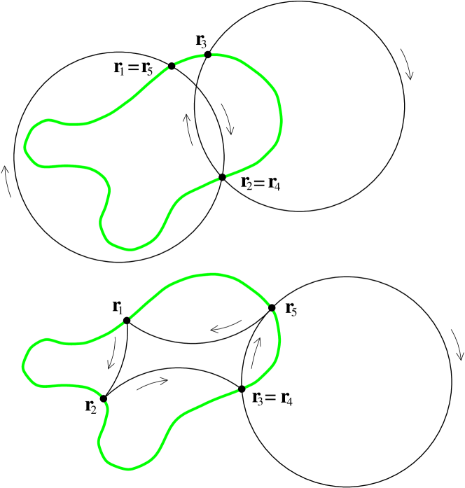
Figure 6.3: Typical saddle point configurations appearing in the semiclassical evaluation of the trace (6.3). Both correspond to unphysical trajectories. The upper configuration has no relation to an orbit of the classical problem, while the lower one corresponds to a physical trajectory which is dressed by an additional cyclotron loop.

From the fact that (6.41) must be satisfied simultaneously at the $n$ points $\mathbf{r}_{j}$ it follows that any saddle point configuration corresponds to a closed, periodic orbit. However, by no means is this orbit necessarily a physically allowed classical trajectory. Figure 6.3 sketches the two different types of saddle point configurations which appear in magnetic billiards. Here we choose $n=5$, ie, the saddle points correspond to periodic orbits of period $5$. Clearly, both of them are unphysical trajectories. The one on the top features a specular reflection at $\mathbf{r}_{2}$. Then the boundary is penetrated at $\mathbf{r}_{3}$ giving rise to a full cyclotron loop. After one more reflection (this time from the exterior) at $\mathbf{r}_{4}=\mathbf{r}_{2}$ the trajectory arrives at its initial point. It performs one more cyclotron orbit without even displaying a boundary point at $\mathbf{r}_{2}$. This saddle point is a legitimate solution of (6.41) belonging to a dense and two-dimensional set of stationary points (since the boundary points $\mathbf{r}_{1}$ and $\mathbf{r}_{2}$ may be shifted independently without changing the picture.) It has clearly no relation to a physical periodic orbit. The saddle point shown on the bottom part of Fig. 6.3, on the other hand, does exhibit the boundary points of a physical periodic orbit (with period 4). Nonetheless, the depicted trajectory is unphysical since it leaves the interior domain, performing a cyclotron loop between the third and forth boundary points. Obviously, there is an infinite number of these unphysical saddle points attached to any proper, physical periodic orbit. They merely dress the original orbit with additional cyclotron loops. It might be expected that these unphysical contributions can be re-summed, leaving behind only the contributions of physical periodic orbits of the interior and exterior problem. This is a difficult task, due to its combinatorial nature in conjunction with a number of ambiguities. A saddle point configuration may, for example, incorporate an interior and and exterior periodic orbit at the same time, leaving the question undetermined whether to assign the contribution to the interior or to the exterior problem. These problems are resolved immediately by the splitting of the operator (6.2) into interior and exterior types. Here, it is the Heaviside functions introduced by the splitting which guarantee that only those saddle points contribute for which the corresponding classical trajectory is directed into the correct domain at each point of reflection. As a consequence, the unphysical solutions discussed above are erased from the sum. The remaining saddle points will be denoted by ${\smash{\gamma_{\rm\,int}^{(n)}}}$ and ${\smash{\gamma_{\rm ext}^{(n)}}}$, respectively. They correspond to the periodic orbits of period $n$ found in the classical interior and exterior billiard problem.

Strictly speaking, the set of saddle points ${\smash{\gamma^{(n)}}}$ which are directed into the correct domain at each point of reflection still includes the so-called ghost orbits. These are periodic orbits which leave (and necessarily re-enter) the proper domain without exhibiting a component of the saddle point (ie, a point of reflection) when leaving it. The left side of Fig. 6.4 shows the situation. Like in the case of non-magnetic billiards [114] these saddle points finally do not contribute to the sum over the traces. This is because for any ghost orbit of period $n$ one finds another of period $n+1$, with an additional boundary point at the position of re-entrance (right side of Fig. 6.4). These two contributions differ by a factor $(-1)$ due to the additional boundary point and therefore cancel.

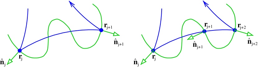
Figure 6.4: Sketch of an interior ghost orbit, see text. (The normals are pointing outwards.)

6.3.2 The prefactors

The next step is to transform the prefactors in the trace integral (6.3). Eventually they should combine with the determinant of the matrix of action derivatives introduced by the stationary phase approximation (A.30). The resulting expression should then be given in terms of the physical properties of the attributed periodic orbit ${\smash{\gamma^{(n)}}}$.

We start with the evaluation of the mixed derivatives of the actions in terms of the angles (6.32), (6.33) characterizing the $j$th part of the trajectory. If the arc is of the short type one obtains the formula

$$\frac{\mathrm{d}^{2}}{\mathrm{d}s_{j}\mathrm{d}s_{j+1}}\,{\rm a}_{\rm S}(s_{j+1},s_{j}) =\frac{1}{\pi\rho}\frac{\mathrm{d}}{\mathrm{d}s_{j+1}}\left(\cos(\alpha_{j})\sin(\beta^{0}_{j})-\frac{\mathbf{r}_{j+1}\,\hat{\mathbf{n}}_{j}}{2\rho}\right)$$

$$=\frac{1}{2\pi\rho^{2}}\Big{(}\tan(\alpha_{j})\sin(\beta_{j+1})\sin(\beta^{0}_{j})$$

$$\phantom{=\frac{1}{2\pi\rho^{2}}\Big{(}}-\cot(\alpha_{j})\cos(\beta_{j+1})\cos(\beta^{0}_{j})+\sin(\beta_{j+1}-\beta^{0}_{j})\Big{)}$$

$$=\frac{-1}{2\pi\rho^{2}}\,\frac{(\hat{\mathbf{v}}^{0}_{{\rm S}\,j}\hat{\mathbf{n}}_{j})(\hat{\mathbf{v}}_{{\rm S}\,j+1}\hat{\mathbf{n}}_{j+1})}{\sin(\alpha_{j})\cos(\alpha_{j})}\ .$$ (6.42)

Here, the expressions given in (6.37) and Tab. 6.1 were employed, as well as

$$\frac{\mathrm{d}}{\mathrm{d}s_{j+1}}\cos(\alpha_{j}) =-\sin(\alpha_{j})\,\frac{\mathrm{d}}{\mathrm{d}s_{j+1}}\arcsin\left(\frac{|\mathbf{r}_{j+1}-\mathbf{r}_{j}|}{2\rho}\right)$$ (6.43)

$$=\frac{-1}{2\rho}\,\frac{\sin(\alpha_{j})}{\cos(\alpha_{j})}\,\frac{(\mathbf{r}_{j+1}-\mathbf{r}_{j})\,\hat{\mathbf{t}}_{j+1}}{|\mathbf{r}_{j+1}-\mathbf{r}_{j}|}=\frac{1}{2\rho}\,{\tan(\alpha_{j})}\sin(\beta_{j+1})$$

and

$$\frac{\mathrm{d}}{\mathrm{d}s_{j+1}}\sin(\beta^{0}_{j}) =\frac{\mathrm{d}}{\mathrm{d}s_{j+1}}\left[\frac{(\mathbf{r}_{j+1}-\mathbf{r}_{j})\times\hat{\mathbf{n}}_{j}}{|\mathbf{r}_{j+1}-\mathbf{r}_{j}|}\right]$$

$$=\frac{\hat{\mathbf{t}}_{j+1}\times\hat{\mathbf{n}}_{j}}{|\mathbf{r}_{j+1}-\mathbf{r}_{j}|}-\frac{(\mathbf{r}_{j+1}-\mathbf{r}_{j})\times\hat{\mathbf{n}}_{j}}{|\mathbf{r}_{j+1}-\mathbf{r}_{j}|}\,\frac{(\mathbf{r}_{j+1}-\mathbf{r}_{j})\,\hat{\mathbf{t}}_{j+1}}{(\mathbf{r}_{j+1}-\mathbf{r}_{j})^{2}}$$

$$=\frac{-1}{2\rho}\,\frac{\cos(\beta_{j+1})\cos(\beta^{0}_{j})}{\sin(\alpha_{j})}\ .$$ (6.44)

Hence, the mixed derivative (6.3.2) is essentially determined by the normal components of the velocities at the initial and the final point of the corresponding arc. Note that this expression is manifestly positive if the arc is part of a physical trajectory meaning that it lies either in the interior or in the exterior at both points (see also Fig. 6.2).

If the $j$th part of the action corresponds to a long arc one obtains in a similar fashion

$$\frac{\mathrm{d}^{2}}{\mathrm{d}s_{j}\mathrm{d}s_{j+1}}\,{\rm a}_{\rm L}(s_{j+1},s_{j}) =\frac{1}{2\pi\rho^{2}}\,\frac{\cos(\beta^{0}_{j}+\alpha_{j})\cos(\beta_{j+1}-\alpha_{j})}{\sin(\alpha_{j})\cos(\alpha_{j})}$$

$$=\frac{1}{2\pi\rho^{2}}\,\frac{(\hat{\mathbf{v}}^{0}_{{\rm L}\,j}\hat{\mathbf{n}}_{j})(\hat{\mathbf{v}}_{{\rm L}\,j+1}\hat{\mathbf{n}}_{j+1})}{\sin(\alpha_{j})\cos(\alpha_{j})}\ .$$ (6.45)

The form of this formula is analogous to (6.3.2), except for the difference in sign. It follows that equation (6.3.2) is manifestly negative if the angles $\alpha_{j},\beta^{0}_{j},$ and $\beta_{j+1}$ describe a segment of a physical trajectory — again due to the change in the orientation of the velocity vector.

The mixed derivatives (6.3.2) and (6.3.2) allow the transformation of the product under the trace integral (6.3) into a symmetrized expression. For a given saddle point ${\smash{\gamma^{(n)}}}$ we denote the geometric part of the total action by

$${\rm A}({\smash{\gamma^{(n)}}}) :=\sum_{j=1}^{n}{\rm a}_{\eta_{j}}(s_{j+1},s_{j})\ ,$$ (6.46)

cf (6.1), (6.2). In addition, the number of long arcs appearing in ${\smash{\gamma^{(n)}}}$ will be called $\ell_{\gamma}$. The product under the trace integral (6.3) can now be stated in terms of ${\rm A}({\smash{\gamma^{(n)}}})$ and $\ell_{\gamma}$. For the interior operators, it assumes the form

$$\mathrm{e}^{2\pi\mathrm{i}\nu{\rm A}({\smash{\gamma_{\rm\,int}^{(n)}}})}\,\mathrm{e}^{-\mathrm{i}\frac{\pi}{2}\ell_{\gamma}}\,\prod_{j=1}^{n}\frac{-(\hat{\mathbf{v}}^{0}_{\eta_{j}}\hat{\mathbf{n}}_{0})_{j}}{\big{(}\sin(\alpha_{j})\cos(\alpha_{j})\big{)}^{\frac{1}{2}}}$$ (6.47)

$$=\, \frac{\prod_{j=1}^{n}\left((\hat{\mathbf{v}}^{0}_{\{\eta_{j}\,j\}}\hat{\mathbf{n}}_{j})(\hat{\mathbf{v}}^{0}_{\{\eta_{j+1}\,j+1\}}\hat{\mathbf{n}}_{j+1})\right)^{\frac{1}{2}}}{\prod_{j=1}^{n}\left(\sin(\alpha_{j})\cos(\alpha_{j})\right)^{\frac{1}{2}}}\,\mathrm{e}^{-\mathrm{i}\frac{\pi}{2}\ell_{\gamma}}\,\mathrm{e}^{2\pi\mathrm{i}\nu{\rm A}({\smash{\gamma_{\rm\,int}^{(n)}}})}$$ (6.47a)

$$=\, \frac{\prod_{j=1}^{n}\left(-(\hat{\mathbf{v}}^{0}_{\{\eta_{j}\,j\}}\hat{\mathbf{n}}_{j})(\hat{\mathbf{v}}_{\{\eta_{j+1}\,j+1\}}\hat{\mathbf{n}}_{j+1})\right)^{\frac{1}{2}}}{\prod_{j=1}^{n}\left(\sin(\alpha_{j})\cos(\alpha_{j})\right)^{\frac{1}{2}}}\,\mathrm{e}^{-\mathrm{i}\frac{\pi}{2}\ell_{\gamma}}\,\mathrm{e}^{2\pi\mathrm{i}\nu{\rm A}({\smash{\gamma_{\rm\,int}^{(n)}}})}$$ (6.47b)

$$=\, \prod_{j=1}^{n}\left(2\pi\rho^{2}\frac{\mathrm{d}^{2}{\rm a}_{\eta_{j}}(s_{j+1},s_{j})}{\mathrm{d}s_{j}\mathrm{d}s_{j+1}}\right)^{\frac{1}{2}}\,\mathrm{e}^{\mathrm{i}\frac{\pi}{2}(\ell_{\gamma}-\ell_{\gamma})}\,\,\mathrm{e}^{2\pi\mathrm{i}\nu{\rm A}({\smash{\gamma_{\rm\,int}^{(n)}}})}$$ (6.47c)

$$=\, (2\pi)^{\frac{n}{2}}\prod_{j=1}^{n}\left|\rho^{2}\frac{\mathrm{d}^{2}{\rm A}({\smash{\gamma_{\rm\,int}^{(n)}}})}{\mathrm{d}s_{j}\mathrm{d}s_{j+1}}\right|^{\frac{1}{2}}\,\mathrm{e}^{-\mathrm{i}\frac{\pi}{2}\ell_{\gamma}}\,\mathrm{e}^{2\pi\mathrm{i}\nu{\rm A}({\smash{\gamma_{\rm\,int}^{(n)}}})}\ .$$ (6.47d)

Here we used several times the fact that the saddle point configurations described by ${\smash{\gamma_{\rm\,int}^{(n)}}}$ correspond to physical, interior periodic orbit with $n$ reflections. First, we noted the positivity of the factor $-(\hat{\mathbf{v}}^{0}_{\eta_{j}}\hat{\mathbf{n}}_{0})_{j}$ to write it as a product of square roots (and shifted one index by one). Second, the reflection condition

$$(\hat{\mathbf{v}}^{0}_{\{\eta_{j}\,j\}}\hat{\mathbf{n}}_{j})=-(\hat{\mathbf{v}}_{\{\eta_{j}\,j\}}\hat{\mathbf{n}}_{j})$$ (6.48)

was employed to get from (6.47a) to (6.47b). As a result, the prefactors are symmetric in $s_{j}$ and $s_{j+1}$, which allows stating them in terms of the mixed derivatives of the classical action. Finally, given the sign of each factor in (6.47d) the sign of the product can be taken out. It is $(-)^{\ell_{\gamma}}$, due to the $\ell_{\gamma}$ long arcs in ${\smash{\gamma^{(n)}}}$.

Upon evaluating the trace of the exterior operators one is led to the same expression (6.47d), with ${\smash{\gamma_{\rm\,int}^{(n)}}}$ replaced by ${\smash{\gamma_{\rm ext}^{(n)}}}$. This is because the additional sign in the definition (6.2) of the exterior operators cancels the change in the orientation of the normals relative to the velocity vectors.

$\rho$ cyclotron radius ($\rho>0$) (2.33) $\alpha$ relative distance of the initial and the final point ($0\leq\alpha\leq\frac{\pi}{2}$) (6.5) $\beta^{0}$ relative direction of normal at the initial point ($0\leq\beta^{0}<2\pi$) (6.6) $\beta$ relative direction of normal at final point ($0\leq\beta<2\pi$) (6.6) ${\rm a}_{\rm S}$, ${\rm a}_{\rm L}$ geometric part of the action of a short (long) arc (6.1) ${\gamma}$, ${\smash{\gamma^{(n)}}}$ physical periodic orbit (with $n$ reflections) page 6.3 ${\rm A}({\gamma})$ geometric part of the action of the periodic orbit ${\gamma}$ (6.46) $n_{\gamma}$ ($r_{\gamma}$) number of reflections (repetitions) in ${\gamma}$ page 6.3.3 $\mu_{\gamma}$ Maslov index (number of conjugate points in ${\gamma}$) page 6.3.3 ${\rm M}({\gamma})$ stability matrix of ${\gamma}$ (6.50)

Table 6.2: Important geometric quantities

6.3.3 Performing the trace

Now, with the prefactors written as mixed derivatives of the action in (6.47d) we can follow the standard procedure to derive the semiclassical trace formula. We apply the stationary phase approximation to the $n$-dimensional trace integral. At first, the contributing saddle points are assumed to be isolated. This amounts to the assumption that the corresponding classical billiard dynamics is hyperbolic [3]. The case of an integrable system is treated afterwards.

Combining eqs (6.3) and (6.47), together with (A.30), yields

$$\mathop{\mathrm{tr}}\nolimits\!\left[\big{(}{\sf P}^{\rm int}\big{)}^{n}\right] =\,\sum_{{\gamma}\in\big{\{}{\gamma_{\rm\,int}^{(n)}}\big{\}}}\frac{n}{r_{\gamma}}\,\frac{1}{\rho^{n}}\,\frac{\prod_{j=1}^{n}\left|\rho^{2}\frac{\partial^{2}{\rm A}({\gamma})}{\partial s_{j}\partial s_{j+1}}\right|^{\frac{1}{2}}}{\left|\det\left(\frac{\partial^{2}{\rm A}({\gamma})}{\partial s_{k}\partial s_{l}}\right)_{k,l}\right|^{\frac{1}{2}}}\,\mathrm{e}^{2\pi\mathrm{i}\nu{\rm A}({\gamma})}\,\mathrm{e}^{-\mathrm{i}\frac{\pi}{2}(\ell_{\gamma}+\nu_{\gamma})}$$

$$=\,\sum_{{\gamma}\in\big{\{}{\gamma_{\rm\,int}^{(n)}}\big{\}}}\frac{n}{r_{\gamma}}\,\frac{1}{|\mathop{\mathrm{tr}}\nolimits({\rm M}({\gamma})-2|^{\frac{1}{2}}}\,\mathrm{e}^{2\pi\mathrm{i}\nu{\rm A}({\gamma})}\,\mathrm{e}^{-\mathrm{i}\frac{\pi}{2}\mu_{\gamma}}\ .$$ (6.49)

The factor $n/r_{\gamma}$ appears because the sum is taken over all $n$-periodic orbits of the interior billiard rather than over all contributing saddle points. Each $n$-periodic orbit (with repetition number $r_{\gamma}$ ) corresponds to $n/r_{\gamma}$ distinct saddle points $\underline{s}$, which are related by a cyclic shift of their components. For the last equality in (6.3.3) we used once more the fact that ${\smash{\gamma_{\rm\,int}^{(n)}}}$ is a classical periodic orbit of a billiard problem. This implies a general relation between the derivatives of the generating function of the billiard map ${\rm A}({\smash{\gamma^{(n)}}})$ and the stability matrix ${\rm M}({\smash{\gamma^{(n)}}})$ [120],

$$\det\left[\left(\frac{\partial^{2}{\rm A}({\smash{\gamma^{(n)}}})}{\partial s_{k}\partial s_{l}}\right)_{k,l}\right]=(-)^{n}\big{[}\mathop{\mathrm{tr}}\nolimits{\rm M}({\smash{\gamma^{(n)}}})-2\big{]}\,\prod_{j=1}^{n}\frac{\partial^{2}{\rm A}({\smash{\gamma^{(n)}}})}{\partial s_{j}\partial s_{j-1}}\ .$$ (6.50)

Its modulus was taken to derive (6.3.3). The integer $\mu_{\gamma}:=\ell_{\gamma}+\nu_{\gamma}$ denotes the total number of conjugate points. Here, $\nu_{\gamma}$ is given by the number of negative eigenvalues of the determinant in the dominator. It counts those conjugate points along the trajectory, which are due to the focusing and defocusing effect of the boundary. The remaining, trivial conjugate points, which show up at each long arc (after an angle of $\pi$), are taken into account by $\ell_{\gamma}$.

For later reference, let us mention that the dual partner orbit of ${\smash{\gamma^{(n)}}}$, denoted as ${\smash{\overline{\gamma}^{(n)}}}$, has

$$\mu_{\overline{\gamma}}=2n-\mu_{\gamma}$$ (6.51)

conjugate points: As discussed in Section 3.2.3 the dual orbits consists of the arcs complementary to those of ${\smash{\gamma^{(n)}}}$ and has opposite orientation. From (6.2) we find ${\rm A}({\smash{\overline{\gamma}^{(n)}}})=n-{\rm A}({\smash{\gamma^{(n)}}})$ and it follows that $\nu_{\overline{\gamma}}=n-\nu_{\gamma}$ since every element of the matrix of second derivatives in (6.3.3) is multiplied by $(-1)$. By definition we have $\ell_{\overline{\gamma}}=n-\ell_{\gamma}$ leading to (6.51). Note also that the stabilities of dual periodic orbits are equal, $\mathop{\mathrm{tr}}\nolimits{\rm M}({\overline{\gamma}})=\mathop{\mathrm{tr}}\nolimits{\rm M}({\gamma})$, which follows from equation (6.50).

The trace formula for the spectral counting function

Inserting the expression for the trace (6.3.3) into (6.29) we obtain the fluctuating number counting function attributed to the interior map operator.

$${\rm N}_{\rm osc}^{\rm skip(int)} :=\frac{1}{\pi}\mathop{\mathrm{Im}}\nolimits\sum_{n=1}^{\infty}\frac{(\mp)^{n}}{n}\,\mathop{\mathrm{tr}}\nolimits\!\left[\big{(}{\sf P}^{\rm int}\big{)}^{n}\right]$$ (6.52)

$$=\frac{1}{\pi}\mathop{\mathrm{Im}}\nolimits\sum_{n=1}^{\infty}\sum_{{\gamma}\in\big{\{}{\gamma_{\rm\,int}^{(n)}}\big{\}}}\frac{(\mp)^{n}}{r_{\gamma}}\frac{1}{\big{|}\mathop{\mathrm{tr}}\nolimits{\rm M}({\gamma})-2\big{|}^{\frac{1}{2}}}\,\mathrm{e}^{2\pi\mathrm{i}\nu{\rm A}({\gamma})-\mathrm{i}\frac{\pi}{2}\mu_{\gamma}}$$

$$=\frac{1}{\pi}\sum_{{\gamma}\in\{{\gamma_{\rm\,int}}\}}\frac{(\mp)^{n_{\gamma}}}{r_{\gamma}\,\big{|}\mathop{\mathrm{tr}}\nolimits{\rm M}({\gamma})-2\big{|}^{\frac{1}{2}}}\,\sin\left({2\pi\nu{\rm A}({\gamma})-\frac{\pi}{2}\mu_{\gamma}}\right)$$ (6.52a)

It is naturally associated with the interior problem, since the sum includes all periodic orbits $\big{\{}{\gamma_{\rm\,int}}\big{\}}$ of the interior billiard problem (with $n_{\gamma}$ the number of reflections). If we are originally interested in the Dirichlet spectrum of the interior billiard we have to choose the upper sign in (6.52). In this case each reflection is associated with an additional phase shift of $\pi$. The lower sign is to be taken if the spectral problem was originally formulated for the exterior spectrum. In this case (6.52) provides the spurious interior Neumann spectrum which is included by the double layer equation. It differs from the Dirichlet spectrum merely by the fact that there is no phase shift associated with the reflections at the billiard boundary.

The second factor of the spectral function (6.2) yields a number counting function which includes the trace over powers of the exterior operators. In complete analogy to the treatment above one obtains a periodic orbit sum like equation (6.3.3). As the only difference, the sum is over all the periodic orbits ${\gamma_{\rm ext}}$ of the exterior classical billiard map,

$${\rm N}_{\rm osc}^{\rm skip(ext)} :=\frac{1}{\pi}\mathop{\mathrm{Im}}\nolimits\sum_{n=1}^{\infty}\frac{(\pm)^{n}}{n}\,\mathop{\mathrm{tr}}\nolimits\!\left[\big{(}{\sf P}^{\rm ext}\big{)}^{n}\right]$$ (6.53)

$$=\frac{1}{\pi}\sum_{{\gamma}\in\{{\gamma_{\rm ext}}\}}\frac{(\pm)^{n_{\gamma}}}{r_{\gamma}\,\big{|}\mathop{\mathrm{tr}}\nolimits{\rm M}({\gamma})-2\big{|}^{\frac{1}{2}}}\,\sin\left(2\pi\nu{\rm A}({\gamma})-\frac{\pi}{2}\mu_{\gamma}\right)\ .$$ (6.53a)

Like above, an additional phase shift of $\pi$ is associated with each reflection if the original double layer equation was formulated for the same domain as the orbits are taken from (upper sign in (6.53a)). Again there is no shift if the periodic orbit sum represents the spurious solutions of the double layer equation which belong to the complementary domain (lower sign). The fact that the trace formulas for Dirichlet and Neumann boundary conditions differ only by a phase is also known from the theory of non-magnetic quantum billiards [76].

We conclude that for either the interior or the exterior Dirichlet problem the fluctuating number function is given by

$${\rm N}_{\rm osc}^{\rm skip}(\nu)=\frac{1}{\pi}\sum_{{\gamma}}\frac{1}{r_{\gamma}\,\big{|}\mathop{\mathrm{tr}}\nolimits{\rm M}({\gamma})-2\big{|}^{\frac{1}{2}}}\,\sin\left(2\pi\nu{\rm A}({\gamma})-\pi n_{\gamma}-\frac{\pi}{2}\mu_{\gamma}\right)\ ,$$ (6.54)

where the sum is over all periodic orbits in the respective domain.

This final result in complete agreement with the standard trace formulas. One could have used them without the preceeding derivation. However, the exclusion of the non-physical trajectories would remain an act of faith. The derivation above provides a sound basis for the intuitively sound results.

6.3.4 Geometric interpretation

At this point a brief discussion of the geometric meaning of a trajectory’s scaled action is in order. We start with the observation that the actions of short and long arcs are given by identical expressions once the parameter

$$\sigma_{j}:=\frac{(\mathbf{r}_{j+1}-\mathbf{c}_{j})\times(\mathbf{r}_{j+1}-\mathbf{r}_{j})}{\rho\,|\mathbf{r}_{j+1}-\mathbf{r}_{j}|}=\begin{cases}-\cos(\alpha_{j})&\text{if ``short'' arc}\\ +\cos(\alpha_{j})&\text{if ``long'' arc}\end{cases}$$ (6.55)

is introduced to describe the $j$-th arc. Unlike the angle $\alpha_{j}$ (6.32), it is not just a function of $\mathbf{r}_{j}$ and $\mathbf{r}_{j+1}$ but it contains information on the type of the arc through its sign: $\sigma_{j}$ is negative for short arcs and positive for long ones. The geometric parts of the actions of short and long arcs, (6.1) and (6.2), now assume the common form

$${\rm a}(\mathbf{r}_{j+1};\mathbf{r}_{j})=\frac{1}{\pi}\left(\frac{\pi}{2}+\arcsin(\sigma_{j})-\sigma_{j}\sqrt{1-\sigma_{j}^{2}}-\frac{\mathbf{r}_{j+1}\times\mathbf{r}_{j}}{2\rho^{2}}\right)\ ,$$ (6.56)

which is a remarkable simplification. It allows to show immediately that a periodic orbit ${\gamma}$ (of period $n$) exhibits a geometric action (6.46)

$${\rm A}({\smash{\gamma^{(n)}}}) =\sum_{j=1}^{n}{\rm a}(\mathbf{r}_{j+1},\mathbf{r}_{j})=\frac{\rho\,\mathrsfs{L}_{\gamma}\pm\mathrsfs{A}_{\gamma}}{\rho^{2}\pi}\ ,$$ (6.57)

which is given by the length of the trajectory,

$$\mathrsfs{L}_{\gamma} :=\rho\sum_{j=1}^{n}\left({\pi}+2\arcsin(\sigma_{j})\right)$$ (6.58)

$$=\rho\,\frac{\mathrm{d}}{\mathrm{d}\nu}\big{[}2\pi\nu{\rm A}({\smash{\gamma^{(n)}}})\big{]}\ ,$$ (6.58a)

and the enclosed area,

$$\mathrsfs{A}_{\gamma} :=\mathrsfs{A}^{\rm poly}_{\gamma}\mp\sum_{j=1}^{n}\left(\frac{\pi}{2}+\arcsin(\sigma_{j})+\sigma_{j}\sqrt{1-\sigma_{j}^{2}}\right)\rho^{2}\ .$$ (6.59)

Here, $\mathrsfs{A}^{\rm poly}_{\gamma}$ is the area of the polygon defined by the points of reflection $\{\mathbf{r}_{j}\}$ and each of the summands in (6.59) is equal to the area enclosed by the $j$-th arc and the cord connecting its initial and final points, cf (2.44). (Overlapping parts of the enclosed area are counted according to their multiplicity.)

Equation (6.58a) follows bearing in mind that $\rho$ and $\sigma_{i}$ are functions of $\nu$, cf (2.37). It illustrates the fact that the excursion time of a trajectory is given by the derivative of its action with respect to energy. Using the proper scaled energy $\widetilde{E}=2\nu$ (cf the discussion of (2.37)) we obtain the scaled time of flight $\tau_{\gamma}$ of the periodic orbit,

$$\tau_{\gamma}=\frac{\mathrm{d}}{\mathrm{d}(2\nu)}\Big{[}2\pi\nu{\rm A}({\smash{\gamma^{(n)}}})\Big{]}=\sum_{j=1}^{n}\left({\frac{\pi}{2}}+\arcsin(\sigma_{j})\right)\ .$$ (6.60)

Density of skipping states

The formula for the fluctuating part of the density of skipping states (3.15) follows by taking the derivative of the number counting function (6.54) with respect to $\nu$,

$$d_{\rm osc}^{\rm skip}(\nu)=\frac{2}{\pi}\sum_{{\gamma}}\frac{\tau_{\gamma}}{r_{\gamma}\,\big{|}\mathop{\mathrm{tr}}\nolimits{\rm M}({\gamma})-2\big{|}^{\frac{1}{2}}}\,\cos\left(2\pi\nu{\rm A}({\gamma})-\pi n_{\gamma}-\frac{\pi}{2}\mu_{\gamma}\right)\ .$$ (6.61)

It must be emphasized, however, that the applicability of this expression is rather restricted so far. It is valid only for the interior billiard and only if the entire phase space consists of skipping trajectories (ie, for weak fields only). In all other cases any attempt to include the cyclotron contributions “by hand” yields unsatisfactory results [71, 124].

Magnetization density

Another derivative of the action occurs in the definition of the scaled magnetization density (3.26) which was discussed in Sect. 3.4. We find that it is determined by the area $\mathrsfs{A}_{\gamma}$ enclosed by the trajectory (6.59),

$$\left(-b^{2}\frac{\mathrm{d}}{\mathrm{d}b^{2}}-\nu\frac{\mathrm{d}}{\mathrm{d}\nu}\right)\Big{[}2\pi\nu{\rm A}({\gamma})\Big{]}=\pm\frac{2}{b^{2}}\mathrsfs{A}_{\gamma}\ .$$ (6.62)

The semiclassical expression for the fluctuating part of the scaled magnetization density is obtained by applying the derivatives in (6.62) to the trace formula for ${\rm N}_{\rm osc}$, cf (3.26). Assuming that all periodic orbits are isolated and of the skipping type we find

$$\widetilde{{\rm m}}^{\rm osc}(\nu) =\pm{2}\sum_{{\gamma}}\frac{{\mathrsfs{A}_{\gamma}}/({b^{2}\pi})}{r_{\gamma}\,\big{|}\mathop{\mathrm{tr}}\nolimits{\rm M}({\gamma})-2\big{|}^{\frac{1}{2}}}\,\cos\left(2\pi\nu{\rm A}({\gamma})-\pi n_{\gamma}-\frac{\pi}{2}\mu_{\gamma}\right)\ .$$ (6.63)

Hence, compared to the density of skipping states (6.61) each periodic orbit contribution to the scaled magnetization density includes the enclosed area in units of $b^{2}\pi$, ie, the magnetic moment of the classical orbit rather than the scaled time of flight. Again, the expression (6.63) is only applicable for the interior problem at weak fields. The corresponding, less intuitive semiclassical expression for the conventional magnetization at weak fields may be found in [66].

6.4 Trace formula for the integrable case

In the previous section the classical billiard map was assumed to be hyperbolic. We now shift to the other extreme, the disk billiard, which exhibits integrable motion.

6.4.1 The disk billiard

The periodic orbit formula for the density of states in the interior of the magnetic disk was derived recently by Blaschke et al.[71]. These authors used the trace formula by Creagh and Littlejohn [125] to account for the continuous circular symmetry of the disk.

In the following, we derive the trace formula starting from the boundary integral equation. This demonstrates how the integrable case is treated in the framework of the boundary map operators and yields an explicit formula in a straightforward manner. Moreover, the exterior case is easily included in our treatment.

Many results of the last section still apply. In particular, the factorization of the spectral function (6.2) does not depend on the type of motion, hence, we can start directly with the equations (6.52) and (6.53) for the interior and the exterior counting functions. However, the trace of powers of the map operators cannot be evaluated like in the hyperbolic case since the periodic orbits are not isolated but appear in continuous families [113].

The classical motion is governed by one parameter, the ratio

$$\Gamma_{\!\rm d}:=\frac{R}{\rho}$$ (6.64)

between the radius of the disk $R$ and the cyclotron radius. For weak fields, $\Gamma_{\!\rm d}<1$, any two points on the boundary can be connected in the interior only by short arcs and in the exterior (only) by long ones. The field is strong, $\Gamma_{\!\rm d}>1$, if complete cyclotron orbits fit into the interior. The skipping motion then displays both types of arcs in the interior and the exterior, and two points on the boundary are no longer necessarily connected by an arc.

It is advantageous to use the polar angles $\varphi=s/R$. To be definite, we shall choose the angles always such, that adjacent points differ at most by $\pi$. Simple geometry tells that the positive angle $\alpha$, as defined in (6.5), obeys

$$\sin(\alpha)=\Gamma_{\!\rm d}\sin\!\left(\frac{|\varphi-\varphi_{0}|}{2}\right).$$ (6.65)

Moreover, we note the relation

$${\frac{1}{2}}\Gamma_{\!\rm d}^{2}\,|\sin(\varphi-\varphi_{0})|\,\gtrless\,\sin(\alpha)\cos(\alpha)\quad\text{for}\quad\Gamma_{\!\rm d}\,\gtrless\,1$$ (6.66)

which is needed in proving almost all the equations below. Finally, geometry tells that the normal components of the reflected velocities are given by

$$-\hat{\mathbf{v}}^{0}_{\left(\begin{smallmatrix}{\rm S}\\ {\rm L}\end{smallmatrix}\right)}\,\hat{\mathbf{n}}_{0}=\frac{1}{\Gamma_{\!\rm d}}\left({\frac{1}{2}}\Gamma_{\!\rm d}^{2}\sin(\varphi-\varphi_{0})\pm\sin(\alpha)\cos(\alpha)\right)\ ,$$ (6.67)

for the short arc and long arc, respectively. They allow stating the prefactors of the map operators (6.20) and (6.21) explicitely in terms of the angle increment $\varphi-\varphi_{0}$.

6.4.2 Operators for the integrable map

Upon choosing the symmetric gauge, ${\raisebox{0.43057pt}{\large$\chi$}}=0$, one finds that the actions of short and long arcs are merely functions of the difference of the initial and the final coordinate,

$${\rm a}_{\rm S}(\varphi-\varphi_{0}):={\rm a}_{\rm S}(R\varphi;R\varphi_{0})=\frac{1}{\pi}\left(\alpha+\sin(\alpha)\cos(\alpha)+\tfrac{1}{2}\Gamma_{\!\rm d}^{2}\sin(\varphi-\varphi_{0})\right)\ ,$$ (6.68)

and likewise ${\rm a}_{\rm L}(\varphi-\varphi_{0}):={\rm a}_{\rm L}(R\varphi;R\varphi_{0})=1-{\rm a}_{\rm S}(\varphi_{0}-\varphi)$. This reflects the integrability of the classical motion.

For the special case of the disk billiard the map operators (6.2) can be related directly to the magnetic generalization of the ${\sf T}$ operator [116]. Following [116] we define two operators, ${\sf T}_{\rm S}$ and ${\sf T}_{\rm L}$, entirely in terms of the actions of a short and long arc, $\eta\in\{{\rm S,L}\}$, respectively, with kernels

$${\rm t}_{\rm\eta}(\varphi;\varphi_{0}) :=\frac{1}{(2\pi\mathrm{i})^{\frac{1}{2}}}\,\left(\frac{\mathrm{d}^{2}(2\pi\nu{\rm a}_{\rm\eta})}{\mathrm{d}\varphi\,\mathrm{d}\varphi_{0}}(\varphi-\varphi_{0})\right)^{\frac{1}{2}}\,\mathrm{e}^{2\pi\mathrm{i}\nu{\rm a}_{\rm\eta}}\ .$$ (6.69)

Evaluating the mixed second derivatives of the actions, one finds that they may be stated in a form

$$\frac{\mathrm{d}^{2}{\rm a}_{\rm S}}{\mathrm{d}\varphi\,\mathrm{d}\varphi_{0}}(\varphi-\varphi_{0}) =\,\phantom{-}\frac{1}{2\pi}\,\frac{(\sin(\alpha)\cos(\alpha)+{\frac{1}{2}}\Gamma_{\!\rm d}^{2}\sin(\varphi-\varphi_{0}))^{2}}{\sin(\alpha)\cos(\alpha)}$$ (6.70)

$$\frac{\mathrm{d}^{2}{\rm a}_{\rm L}}{\mathrm{d}\varphi\,\mathrm{d}\varphi_{0}}(\varphi-\varphi_{0}) =\,-\frac{1}{2\pi}\,\frac{(\sin(\alpha)\cos(\alpha)-{\frac{1}{2}}\Gamma_{\!\rm d}^{2}\sin(\varphi-\varphi_{0}))^{2}}{\sin(\alpha)\cos(\alpha)}$$ (6.71)

which permits the direct comparison with equation (6.67). It follows that the operators ${\sf P}_{\rm S}^{\rm int}$ and ${\sf P}_{\rm S}^{\rm ext}$ (cf eq (6.2)) are given essentially in terms of ${\sf T}_{\rm S}$:

$${\rm p}_{\rm S}^{\rm int}(R\varphi,R\varphi_{0}) ={\rm t}_{\rm S}\left(\varphi;\varphi_{0}\right)\,\frac{b}{R}\,\begin{cases}\Theta(\varphi-\varphi_{0})&\text{if $\Gamma_{\!\rm d}>1$}\\ 1&\text{if $\Gamma_{\!\rm d}<1$}\end{cases}$$ (6.72)

$${\rm p}_{\rm S}^{\rm ext}(R\varphi,R\varphi_{0}) ={\rm t}_{\rm S}\left(\varphi;\varphi_{0}\right)\,\frac{b}{R}\,\begin{cases}\Theta(\varphi_{0}-\varphi)&\text{if $\Gamma_{\!\rm d}>1$}\\ 0&\text{if $\Gamma_{\!\rm d}<1$}\end{cases}$$ (6.73)

They vanish whenever there is no classically allowed trajectory connecting the initial and the final point in the considered domain. Similarly, the operators ${\sf P}_{\rm L}^{\rm int}$ and ${\sf P}_{\rm L}^{\rm ext}$ are given as restrictions of ${\sf T}_{\rm L}$.

$${\rm p}_{\rm L}^{\rm int}(R\varphi,R\varphi_{0}) =-{\rm t}_{\rm L}\left(\varphi;\varphi_{0}\right)\,\frac{b}{R}\,\begin{cases}\Theta(\varphi-\varphi_{0})&\text{if $\Gamma_{\!\rm d}>1$}\\ 0&\text{if $\Gamma_{\!\rm d}<1$}\end{cases}$$ (6.74)

$${\rm p}_{\rm L}^{\rm ext}(R\varphi,R\varphi_{0}) =-{\rm t}_{\rm L}\left(\varphi;\varphi_{0}\right)\,\frac{b}{R}\,\begin{cases}\Theta(\varphi_{0}-\varphi)&\text{if $\Gamma_{\!\rm d}>1$}\\ 1&\text{if $\Gamma_{\!\rm d}<1$}\end{cases}$$ (6.75)

Here we assume $|\varphi-\varphi_{0}|\leq\pi$ (as throughout this section).

6.4.3 The explicit trace formula

To obtain a semiclassical expression for the number counting function we start by calculating the kernel of the $N$th power $({\sf P}^{\rm int})^{N}$ at coinciding initial and final point $s_{0}$. It is given by a $(N-1)$-dimensional integral,

$$\left({\rm p}^{\rm int}\right)^{N}(s_{0},s_{0}) =\int\prod_{j=1}^{N}\left[\big{(}{\rm p}_{\rm S}^{\rm int}+{\rm p}_{\rm L}^{\rm int}\big{)}(s_{j},s_{j-1})\right]\frac{\mathrm{d}s_{1}\ldots\mathrm{d}s_{N-1}}{b^{N-1}}\ ,$$ (6.76)

with fixed $s_{N}\equiv s_{0}$. This integral may be evaluated by the stationary phase method. For the same reason as above (Sect. 6.3.1) only the saddle points contribute which correspond to a physically allowed trajectory. However, they are now required to start and end at the point $s_{0}$. Each saddle point is characterized by the constant angular increment $\Delta\varphi$, the $j$th component given by

$$\varphi_{j}=\varphi_{0}+j\,\Delta\varphi\ ,\qquad j=0,\ldots,N-1\ .$$ (6.77)

For given $N$ there is a finite number of possible increments

$$\Delta\varphi\in\mathcal{P}_{\rm int}^{N}=\begin{cases}+2\pi\frac{M}{N};\quad M=1,2,\ldots M_{\rm max}&\text{if $\Gamma_{\!\rm d}>1$}\\ \pm 2\pi\frac{M}{N};\quad M=1,2,\ldots M_{\rm max}&\text{if $\Gamma_{\!\rm d}<1$.}\end{cases}$$ (6.78)

Here, the second index $M$ has the meaning of a winding number. It gives the number of times the trajectory encircles the origin. The maximum value is given by

$$M_{\rm max}=\begin{cases}[\arcsin(1/\Gamma_{\!\rm d})\,N/\pi]&\text{if $\Gamma_{\!\rm d}>1$}\\ \quad\quad[N/2]&\text{if $\Gamma_{\!\rm d}<1$,}\end{cases}$$ (6.79)

where $[\cdot]$ indicates the integer part. The stationary phase approximation (A.30) brings about a ($N-1$)-dimensional matrix of second derivatives. Its determinant is easily calculated since the difference between adjacent angles is constant:

$$\det\left(\frac{\partial^{2}\sum{\rm a}(\varphi_{j+1}-\varphi_{j})}{\partial\varphi_{k}\partial\varphi_{l}}\right)_{k,l=1\ldots N-1}\!\!= \,\left({\rm a}^{\prime\prime}(\Delta\varphi)\right)^{N-1}\,\det\begin{pmatrix}\textstyle 2&-1&&0\\ \textstyle-1&\ddots&\ddots&\\ \textstyle&\ddots&\ddots&-1\\ \textstyle 0&&-1&2\end{pmatrix}$$

$$= \,N\,\left({\rm a}^{\prime\prime}(\Delta\varphi)\right)^{N-1}$$ (6.80)

The number of negative eigenvalues is $\nu_{\sf A}=0$ or $\nu_{\sf A}=N-1$, respectively, for positive or negative sign of ${\rm a}^{\prime\prime}(\Delta\varphi)$ (ie, for long or short arcs).

Taking the square-root of (6.4.3) cancels all but one of the prefactors in the integrand of eq (6.76). Altogether, the kernel $\left({\rm p}_{\rm S}^{\rm int}+{\rm p}_{\rm L}^{\rm int}\right)^{N}(s_{0},s_{0})$ is given by

$$\frac{1}{(2\pi\mathrm{i})^{\frac{1}{2}}}\,\frac{1}{\sqrt{N}}\frac{b}{R}\sum_{\Delta\varphi\in\mathcal{P}_{\rm int}^{N}}\bigg{\{} \left|\frac{\mathrm{d}^{2}(2\pi\nu{\rm a}_{\rm S}(\Delta\varphi))}{\mathrm{d}\varphi^{2}}\right|^{\frac{1}{2}}\mathrm{e}^{N2\pi\mathrm{i}\nu{\rm a}_{\rm S}(\Delta\varphi)-\mathrm{i}\frac{\pi}{2}(N-1)}$$ (6.81)

$$+ \left|\frac{\mathrm{d}^{2}(2\pi\nu{\rm a}_{\rm L}(\Delta\varphi))}{\mathrm{d}\varphi^{2}}\right|^{\frac{1}{2}}\mathrm{e}^{N2\pi\mathrm{i}\nu{\rm a}_{\rm L}(\Delta\varphi)-\mathrm{i}\frac{\pi}{2}N}\,\Theta(\Gamma_{\!\rm d}-1)\bigg{\}}\ .$$

It is a sum over all families of interior periodic orbits where each family is represented by the orbit starting at $s_{0}$.

The $n$th power of the exterior operators, $({\sf P}_{\rm S}^{\rm ext}+{\sf P}_{\rm L}^{\rm ext})^{N}$, assumes the same form except for the Heaviside function which appears in the short arc term of the sum. Naturally, the summation is now over the exterior periodic orbit families, the respective increments given by the set

$$\mathcal{P}_{\rm ext}^{N}=\begin{cases}-2\pi\frac{M}{N};\quad M=1,2,\ldots M_{\rm max}&\text{if $\Gamma_{\!\rm d}>1$}\\ \pm 2\pi\frac{M}{N};\quad M=1,2,\ldots M_{\rm max}&\text{if $\Gamma_{\!\rm d}<1$\ .}\end{cases}$$ (6.82)

As the last step in forming the trace $\mathop{\mathrm{tr}}\nolimits\{({\sf P}^{\rm int})^{N}\}$ we have to integrate $s_{0}$. Since the expression (6.81) does not depend on $s_{0}$ this simply adds the factor $2\pi R/b$.

It follows that the fluctuating number function due to the skipping orbits (6.52) assumes the form

$${\rm N}_{\rm osc}^{\rm skip(int)} =\left(\frac{2\nu}{\pi}\right)^{\frac{1}{2}}\sum_{N=2}^{\infty}\,\frac{1}{N^{3/2}}\sum_{\Delta\varphi\in\mathcal{P}_{\rm int}^{N}}\bigg{\{}$$ (6.83)

$$\begin{aligned} &\frac{{\frac{1}{2}}\Gamma_{\!\rm d}^{2}\sin(\Delta\varphi)+\sin(\alpha)\cos(\alpha)}{(\sin(\alpha)\cos(\alpha))^{\frac{1}{2}}}\sin\left(2\pi\nu N\,{\rm a}_{\rm S}(\Delta\varphi)+N\frac{\pi}{2}+\frac{\pi}{4}\right)\\ +&\frac{{\frac{1}{2}}\Gamma_{\!\rm d}^{2}\sin(\Delta\varphi)-\sin(\alpha)\cos(\alpha)}{(\sin(\alpha)\cos(\alpha))^{\frac{1}{2}}}\sin\left(2\pi\nu N\,{\rm a}_{\rm L}(\Delta\varphi)+N\frac{\pi}{2}-\frac{\pi}{4}\right)\Theta(\Gamma_{\!\rm d}-1)\bigg{\}},\end{aligned}$$

with $\alpha\equiv\arcsin(\Gamma_{\!\rm d}\sin(|\Delta\varphi|/2))$. Analogously, the periodic orbit sum for the exterior problem is given by

$${\rm N}_{\rm osc}^{\rm skip(ext)} =\left(\frac{2\nu}{\pi}\right)^{\frac{1}{2}}\sum_{N=2}^{\infty}\,\frac{1}{N^{3/2}}\sum_{\Delta\varphi\in\mathcal{P}_{\rm ext}^{N}}\bigg{\{}$$ (6.84)

$$\begin{aligned} -&\frac{\sin(\alpha)\cos(\alpha)+{\frac{1}{2}}\Gamma_{\!\rm d}^{2}\sin(\Delta\varphi)}{(\sin(\alpha)\cos(\alpha))^{\frac{1}{2}}}\sin\left(2\pi\nu N\,{\rm a}_{\rm S}(\Delta\varphi)+N\frac{\pi}{2}+\frac{\pi}{4}\right)\Theta(\Gamma_{\!\rm d}-1)\\ +&\frac{\sin(\alpha)\cos(\alpha)-{\frac{1}{2}}\Gamma_{\!\rm d}^{2}\sin(\Delta\varphi)}{(\sin(\alpha)\cos(\alpha))^{\frac{1}{2}}}\sin\left(2\pi\nu N\,{\rm a}_{\rm L}(\Delta\varphi)+N\frac{\pi}{2}-\frac{\pi}{4}\right)\bigg{\}}.\end{aligned}$$

The conventional density of states

The semiclassical expression for the density of states is obtained by taking the derivative of the number function with respect to the energy. In order to compare with the result of Blaschke and Brack, which is in units of the conventional energy $E$, we have to take the derivative

$$\frac{\mathrm{d}}{\mathrm{d}E}=\frac{1}{E}\left(\nu\frac{\mathrm{d}}{\mathrm{d}\nu}-{\frac{1}{2}}\Gamma_{\!\rm d}\frac{\mathrm{d}}{\mathrm{d}\Gamma_{\!\rm d}}\right)\ .$$ (6.85)

Applying this differential to (6.83) yields the fluctuating part of the density for the interior problem

$$d_{\rm osc}^{\rm\,skip(int)}(E)=\frac{1}{E}\frac{(2\nu)^{\frac{3}{2}}}{\pi^{\frac{1}{2}}}\sum_{N=2}^{\infty}\sum_{\Delta\varphi\in\mathcal{P}_{\rm int}^{N}}\frac{1}{\sqrt{N}}$$

$$\times\begin{aligned} \bigg{\{}&\alpha\;\frac{{\frac{1}{2}}\Gamma_{\!\rm d}^{2}\sin(\Delta\varphi)+\sin(\alpha)\cos(\alpha)}{(\sin(\alpha)\cos(\alpha))^{\frac{1}{2}}}\cos\left(2\pi\nu N\,{\rm a}_{\rm S}(\Delta\varphi)+N\frac{\pi}{2}+\frac{\pi}{4}\right)\\ +&{(\pi-\alpha)}\,\frac{{\frac{1}{2}}\Gamma_{\!\rm d}^{2}\sin(\Delta\varphi)-\sin(\alpha)\cos(\alpha)}{(\sin(\alpha)\cos(\alpha))^{\frac{1}{2}}}\cos\left(2\pi\nu N\,{\rm a}_{\rm L}(\Delta\varphi)+N\frac{\pi}{2}-\frac{\pi}{4}\right)\Theta(\Gamma_{\!\rm d}-1)\bigg{\}}\ .\end{aligned}$$

This periodic orbit formula is identical to the result in [71]. It approximates the quantum spectrum of the interior magnetic disk only for weak fields $\Gamma_{\!\rm d}<1$, when all trajectories are of the skipping type. For strong fields, $\Gamma_{\!\rm d}>1$, complete cyclotron orbits occur in the interior. One might wish to include the latter “by hand” into the periodic orbit sum. However, it was shown in [71] that energies close to the Landau levels cannot be reproduced this way. Rather than trying to refine the semiclassical approximation, we shall define a new spectral density of edge states below which will resolve the problem of the bulk contributions.

6.5 The separable case

We proceed to quantize the disk billiard for a second time – now using the separability of the quantum problem in a specific gauge. This way closed expressions for the spectral functions may be obtained, which yield explicit formulas for important quantities, such as the magnetization. Moreover, by formulating the relation to the periodic orbit formula derived in the preceeding section we can examine the effect of general boundary conditions on the trace formula.

6.5.1 The disk billiard revisited

The magnetic disk turns into a separable problem if we choose the symmetric gauge, ${\raisebox{0.43057pt}{\large$\chi$}}=0$, and place the center of the disk at the origin. In this case the canonical angular momentum $L$ is conserved and the eigenstates are characterized by the quantum number

$$m=\frac{L}{\hbar}=\frac{c^{2}-\rho^{2}}{b^{2}}\ .$$ (6.87)

In the second part of (6.87) we state the scaled angular momentum in terms of the radial distance $c$ of the center of motion, cf (2.12). Along with the cyclotron radius $\rho$ the latter determines whether the classical motion is of the skipping type. This is the case for $R-\rho<c<R+\rho$. Hence, a quantum state (of energy $\nu$) corresponds to classically skipping motion if its angular momentum quantum number $m$ is bounded from above and below by

$$m_{\rm max} ={\widetilde{R}}^{2}+2\sqrt{\nu}{\widetilde{R}}$$ (6.88)

and

$$m_{\rm min} =\max\big{(}{\widetilde{R}}^{2}-2\sqrt{\nu}{\widetilde{R}},-\nu\big{)}\ ,$$ (6.88a)

respectively. Here, the scaled radius ${\widetilde{R}}:=R/b$ enters as the only external parameter.

We start with the traditional Bohr-Sommerfeld quantization method and proceed to discuss its relation to the periodic orbit formula of Sect. 6.4. The exact quantization in terms of special functions is discussed in Appendix A.3.

6.5.2 Semiclassical quantization

Using polar coordinates $(r,\vartheta)$, the ansatz

$$\psi(r,\vartheta)=\frac{\varphi(r/b)}{\sqrt{r/b}}\,\mathrm{e}^{\mathrm{i}m\vartheta}$$ (6.89)

transforms equation (4.1) into the form of a one-dimensional Schrödinger equation for the radial function $\varphi({\tilde{r}})$.

$$-\frac{1}{4}\varphi^{\prime\prime}({\tilde{r}})+\left(\frac{1}{4}\frac{({\tilde{r}}^{2}-m)^{2}-\frac{1}{4}}{{\tilde{r}}^{2}}-\nu\right)\varphi({\tilde{r}})=0$$ (6.90)

It may be solved to leading order in $b^{2}$ using the standard WKB technique, see eg [126, 34].

The semiclassical wave function

It follows that in the energetically allowed region the resulting semiclassical wave function has the form

$$\psi^{\rm(sc)}(r,\vartheta)=\mathcal{N}_{\rm disk}\,\frac{\cos\big{(}\Phi^{\rm int/ext}_{\rm disk}(\nu,m,\frac{r}{b})-\frac{\pi}{4}\big{)}}{\big{(}4\nu\frac{r}{b}-\big{(}(\frac{r}{b})^{2}-m\big{)}^{2}\big{)}^{\frac{1}{4}}}\,\mathrm{e}^{\mathrm{i}m\vartheta}\ .$$ (6.91)

Here, the phases $\Phi^{\rm int}_{\rm disk}$ and $\Phi^{\rm ext}_{\rm disk}$ are obtained by an integration starting at the interior and exterior classical turning points of the radial motion, respectively.

$$\Phi^{\rm int}_{\rm disk}(\nu,m,{\tilde{r}}) ={\frac{1}{2}}\sqrt{4\nu{\tilde{r}}^{2}-({\tilde{r}}^{2}-m)^{2}}-(\nu+\frac{m}{2})\arctan\!\left(\frac{2\nu+m-{\tilde{r}}^{2}}{\sqrt{4\nu{\tilde{r}}^{2}-({\tilde{r}}^{2}-m)^{2}}}\right)$$

$$\phantom{=}-\frac{m}{2}\arctan\!\left(\frac{(2\nu+m){\tilde{r}}^{2}-m^{2}}{m\sqrt{4\nu{\tilde{r}}^{2}-({\tilde{r}}^{2}-m)^{2}}}\right)+\frac{\pi}{2}\left(\nu+\frac{m-|m|}{2}\right)$$ (6.92)

and

$$\Phi^{\rm ext}_{\rm disk}(\nu,m,{\tilde{r}}) =\pi\left(\nu+\frac{m-|m|}{2}\right)-\Phi^{\rm int}_{\rm disk}(\nu,m,{\tilde{r}})\ .$$ (6.93)

As for the normalization factor $\mathcal{N}_{\rm disk}$, we find [126]

$$(\mathcal{N}_{\rm disk})^{-2} :=\frac{\pi^{2}}{4}\mp\frac{\pi}{2}\arctan\!\left(\frac{2\nu+m-{\widetilde{R}}^{2}}{\sqrt{4\nu{\widetilde{R}}^{2}-({\widetilde{R}}^{2}-m)^{2}}}\right)\ ,$$ (6.94)

where again the upper sign stands for the interior problem.

A spectral function

Allowing for general boundary conditions (3.6) at the disk radius $r=R$, we obtain the quantization condition

$$\pm\cot\big{(}\Phi^{\rm int/ext}_{\rm disk}(\nu,m,{\widetilde{R}})-\frac{\pi}{4}\big{)}$$

$$=-\frac{(\pm\Lambda)\,\big{(}{4\nu{\widetilde{R}}^{2}-({\widetilde{R}}^{2}-m)^{2}}\big{)}^{\frac{3}{2}}}{2\sqrt{\nu}{\widetilde{R}}\big{(}{4\nu{\widetilde{R}}^{2}-({\widetilde{R}}^{2}-m)^{2}}\big{)}+(\pm\Lambda){\widetilde{R}}^{2}\big{(}2\nu+m-{\widetilde{R}}^{2}\big{)}}\ .$$ (6.95)

The boundary condition enters on the right side through the dimensionless mixing parameter $\Lambda$ (3.7) which vanishes for Dirichlet boundary conditions. In order to transform the dependence on the boundary condition into a phase shift $\alpha_{\Lambda}$, we define

$$\alpha_{\Lambda}(\nu,m,{\widetilde{R}}):=\arctan\!\left(\frac{(\pm\Lambda)\,\big{(}{4\nu{\widetilde{R}}^{2}-({\widetilde{R}}^{2}-m)^{2}}\big{)}^{\frac{3}{2}}}{2\sqrt{\nu}{\widetilde{R}}\big{(}{4\nu{\widetilde{R}}^{2}-({\widetilde{R}}^{2}-m)^{2}}\big{)}+(\pm\Lambda)\,{\widetilde{R}}^{2}\big{(}2\nu+m-{\widetilde{R}}^{2}\big{)}}\right)$$ (6.96)

The semiclassical quantization condition (6.5) is then readily brought into a form,

$$\cos\Big{(}\Phi^{\rm int/ext}_{\rm disk}(\nu,m,{\widetilde{R}})\mp\alpha_{\Lambda}(\nu,m,{\widetilde{R}})-\frac{\pi}{4}\Big{)}=0\ ,$$ (6.97)

which permits a spectral function $\xi$ to be written in terms of two quantum numbers, the number of radial nodes $n$, and the angular momentum $m$,

$$\xi_{\rm disk}^{\rm(sc)}\Big{(}\nu;n,m,\Lambda,\frac{R}{b}\Big{)}:=\Phi^{\rm int/ext}_{\rm disk}\Big{(}\nu,m,\frac{R}{b}\Big{)}\mp\alpha_{\Lambda}\Big{(}\nu,m,\frac{R}{b}\Big{)}-\Big{(}n+\frac{3}{4}\Big{)}\pi\ ,$$ (6.98)

with $n\in{{{\mathbb{N}}}_{0}},m_{\rm min}\leq m\leq m_{\rm max}$ (6.88). Its zero in $\nu$ yields the semiclassical energy of a state with given radial and angular quantum numbers $n$ and $m$. Although the energies are defined implicitly by (6.98), the spectral function yields explicit formulas for the infinitesimal change of the energies as an external parameter is varied. For the derivative of the energy with respect to the boundary mixing parameter at Dirichlet boundary conditions ($\Lambda=0$) we obtain

$$\left.\frac{\mathrm{d}\nu}{\mathrm{d}\Lambda}\right|_{\Lambda=0}=-\,\frac{\displaystyle\;\frac{\mathrm{d}}{\mathrm{d}\Lambda}\xi_{\rm disk}^{\rm(sc)}\;}{\displaystyle\frac{\mathrm{d}}{\mathrm{d}\nu}\xi_{\rm disk}^{\rm(sc)}} =\frac{\displaystyle\sqrt{1-\frac{({\widetilde{R}}^{2}-m)^{2}}{4\nu{\widetilde{R}}^{2}}}}{\displaystyle\frac{\pi}{2}\mp\arctan\!\left(\frac{2\nu+m-{\widetilde{R}}^{2}}{\sqrt{4\nu{\widetilde{R}}^{2}-({\widetilde{R}}^{2}-m)^{2}}}\right)}\ .$$ (6.99)

This short formula is further compressed below and needed soon.

The magnetic moment

It was shown in Section 3.4 that the scaled magnetic moment of a quantum state in the magnetic billiard is determined by the derivative of its energy with respect to the magnetic length, see (3.25). From the semiclassical spectral function (6.98) we find

$$b^{2}\,\frac{\mathrm{d}\nu}{\mathrm{d}b^{2}}=-\,\frac{\displaystyle b^{2}\,\frac{\mathrm{d}}{\mathrm{d}b^{2}}\xi_{\rm disk}^{\rm(sc)}\;}{\displaystyle\frac{\mathrm{d}}{\mathrm{d}\nu}\xi_{\rm disk}^{\rm(sc)}} =\pm{\frac{1}{2}}\,\frac{\displaystyle\sqrt{4\nu{\widetilde{R}}^{2}-({\widetilde{R}}^{2}-m)^{2}}}{\displaystyle\frac{\pi}{2}\mp\arctan\!\left(\frac{2\nu+m-{\widetilde{R}}^{2}}{\sqrt{4\nu{\widetilde{R}}^{2}-({\widetilde{R}}^{2}-m)^{2}}}\right)}\ .$$ (6.100)

Alternatively, the expectation value may be calculated directly, using the semiclassical wave function (6.91). We obtain indeed, after lengthy transformations,

$${\frac{1}{2}}\langle\psi^{\rm(sc)}|(\tilde{\mathbf{r}}\times\tilde{\mathbf{v}})_{\rm sym}|\psi^{\rm(sc)}\rangle=\int\!\mathop{\mathrm{Im}}\nolimits\Big{[}\psi^{*}_{\rm(sc)}(\partial_{\vartheta}-\mathrm{i}\,{\tilde{r}}^{2})\psi^{\rm(sc)}\Big{]}\,\mathrm{d}\vartheta\,{\tilde{r}}\,\mathrm{d}{\tilde{r}}$$

$$=\pm{\frac{1}{2}}\,\frac{\displaystyle\sqrt{4\nu{\widetilde{R}}^{2}-({\widetilde{R}}^{2}-m)^{2}}}{\displaystyle\frac{\pi}{2}\mp\arctan\!\left(\frac{2\nu+m-{\widetilde{R}}^{2}}{\sqrt{4\nu{\widetilde{R}}^{2}-({\widetilde{R}}^{2}-m)^{2}}}\right)}\,-\,\nu\ ,$$ (6.101)

in agreement with (3.25). In the above radial integration (which is limited by the disk radius and the interior or exterior turning point, respectively), the strongly fluctuating $\cos^{2}$-term was replaced by its mean. The fact that the exact relation (3.25) is reproduced shows that this approximation is consistent with the semiclassical one.

The bulk states

States with angular momenta beyond the bounds given by (6.88) are not included in the spectral function (6.98). Classically, they correspond to cyclotron motion. The semiclassical energies of these bulk states are determined by the condition that the two wave functions (6.91) defined from the interior and exterior turning points must match. They are given by the Landau energies $\nu=n+{\frac{1}{2}}$, and the wave functions are readily shown to exhibit a magnetic moment of $-\nu$.

However, the exact quantization, which is given in Appendix A.3, does not distinguish between edge and bulk states and the bulk energies exhibit deviations from the Landau energies. An asymptotic treatment of these exponential corrections to the bulk energy is given in Sect. 7.3.1.

6.5.3 Relation to the periodic orbit formula

In the preceeding section 6.5.2 the semiclassical quantization was carried out according to the traditional Bohr-Sommerfeld rule for separable systems. It is based on the quantizing tori, ie, those invariant manifolds in phase space whose scaled actions are integers. This should be contrasted to the periodic orbit formula for the magnetic disk derived in Sect. 6.4. The latter is a sum over the rational tori, whose classical frequencies are commensurate [113]. In order to sketch how the trace formula is connected to the Bohr-Sommerfeld quantization we follow the work of Berry and Tabor [112] who derived the trace formula for general integrable systems. In particular, this permits us to show how the trace formula is modified if one allows for general boundary conditions (3.6).

The semiclassical spectrum is given by the energies $\nu(n,m)$, which are implicitly defined as the roots of $\xi_{\rm disk}^{\rm(sc)}$ (6.98). We may write the spectral density as a sum over the two quantum numbers,

$$d(\nu_{0}) =\sum_{n,m}\delta\big{(}\nu_{0}-\nu(n,m)\big{)}$$

$$=\overline{d}(\nu_{0})+{\sum_{N,M=-\infty}^{\infty}}\int\mathrm{e}^{2\pi\mathrm{i}(Nn+Mm)}\delta\big{(}\nu(n,m)-\nu_{0}\big{)}\,\mathrm{d}n\,\mathrm{d}m$$

$$=\overline{d}(\nu_{0})+\sum_{N,M=-\infty}^{\infty}\int\Big{|}\frac{\mathrm{d}n}{\mathrm{d}\nu}\Big{|}\,\mathrm{e}^{2\pi\mathrm{i}(Nn(\nu_{0},m)+Mm)}\,\mathrm{d}m\ ,$$ (6.102)

where the Poisson summation formula (eg [127]) was employed to transform the sum into an integral. (Boundary corrections which are to higher order in $\nu$ are neglected.) The sum excludes the term with $N=M=0$, which yields the mean density $\overline{d}$. Upon integrating $n$ the $\delta$-function selects the real valued “number” of radial nodes which is known explicitely from above.

$$n(\nu_{0},m)=\frac{1}{\pi}\Big{(}\Phi^{\rm int/ext}_{\rm disk}(\nu_{0},m,{\widetilde{R}})\mp\alpha_{\Lambda}(\nu,m,{\widetilde{R}})-\frac{3\pi}{4}\Big{)}$$ (6.103)

We evaluate the remaining integral in (6.102) by the stationary phase approximation. The phase shift $\alpha_{\Lambda}$ should be neglected in the saddle point condition

$$-2\frac{\mathrm{d}}{\mathrm{d}m}\big{[}\Phi^{\rm int/ext}_{\rm disk}\mp\alpha_{\Lambda}\big{]}\,\stackrel{{\scriptstyle!}}{{=}}\,2\pi\frac{M}{N}\equiv\Delta\varphi$$ (6.104)

since $\Phi$ is of order $\nu$ (while $\alpha_{\Lambda}$ is of order $1$). A detailed calculation shows, that the angles $\Delta\varphi$ selected by (6.104) are indeed given by the sets $\mathcal{P}_{\rm int/ext}^{N}$ defined in (6.78) and (6.82) (modulo $2\pi$). It is now convenient to characterize the corresponding skipping trajectories by the signed sine of the angle of incidence

$$\varepsilon:=\frac{c^{2}-R^{2}-\rho^{2}}{2R\rho}=\hat{\mathbf{n}}\times\hat{\mathbf{v}}\ ,$$ (6.105)

such that the former quantum number $m$ is given by the real value

$$m={\widetilde{R}}^{2}+2\sqrt{\nu}{\widetilde{R}}\,\varepsilon\ .$$ (6.106)

One finds, after a lengthy calculation, that

$$2\Phi^{\rm int/ext}_{\rm disk}+\frac{M}{N}2\pi m =\pi\nu+2\nu\arcsin(\sigma)-2\nu\sigma\sqrt{1-\sigma^{2}}+{\widetilde{R}}^{2}\sin(\Delta\varphi)$$

$$=2\pi\nu\,{\rm a}$$ (6.107)

with $\sigma=\mp(\varepsilon R+\rho)/c$ defined in (6.55), and “${\rm a}$” the geometric action (6.56) of one arc. Transforming the summation in (6.102) to positive $N$ we obtain, observing (A.29),

$$d_{\rm osc}^{\rm skip}(\nu_{0})= \,\frac{2}{\sqrt{\pi}}\!\!\!\sum_{\begin{smallmatrix}N\in{{\mathbb{N}}},M\in{{\mathbb{Z}}}:\\ \Delta\varphi=2\pi\frac{M}{N}\in\mathcal{P}^{N}_{\rm int/ext}\end{smallmatrix}}\!\!\!\frac{1}{N^{\frac{1}{2}}}\,\frac{\frac{\mathrm{d}}{\mathrm{d}\nu}\Phi^{\rm int/ext}_{\rm disk}}{\left|\frac{\mathrm{d}^{2}}{\mathrm{d}m^{2}}\Phi^{\rm int/ext}_{\rm disk}\right|^{\frac{1}{2}}}$$ (6.108)

$$\times\cos\Big{(}N2\pi\nu a+N\frac{\pi}{2}+\frac{\pi}{4}\mathop{\mathrm{sgn}}\nolimits\big{(}N\partial_{m}^{2}\Phi^{\rm int/ext}_{\rm disk}\big{)}\mp 2N\alpha_{\Lambda}\Big{)}\ .$$

We note the derivatives

$$\frac{\mathrm{d}^{2}}{\mathrm{d}m^{2}}\Phi^{\rm int/ext}_{\rm disk} =-\frac{1}{2{\widetilde{R}}\tilde{c}}\,\frac{\sigma}{\sqrt{1-\varepsilon^{2}}}$$ (6.109)

and

$$\frac{\mathrm{d}}{\mathrm{d}\nu}\Phi^{\rm int/ext}_{\rm disk} =\frac{\pi}{2}+\arcsin(\sigma)={\frac{1}{2}}\,\frac{\mathrm{d}}{\mathrm{d}\nu}\big{(}2\pi\nu a\big{)}\ .$$ (6.110)

The last equality permits to integrate the spectral density immediately. It yields the oscillatory part of the number counting function,

$${{\rm N}}_{\rm osc}^{\rm skip}(\nu_{0})= \,\Big{(}\frac{2\nu}{\pi}\Big{)}^{\frac{1}{2}}\sum_{N=2}^{\infty}\sum_{\Delta\varphi\in\mathcal{P}^{N}}\frac{1}{N^{\frac{3}{2}}}\,\frac{\left(\frac{Rc}{\rho^{2}}\,\sqrt{1-\varepsilon^{2}}\sqrt{1-\sigma^{2}}\right)^{\frac{1}{2}}}{\left|\sigma\sqrt{1-\sigma^{2}}\right|^{\frac{1}{2}}}$$ (6.111)

$$\times\sin\Big{(}2\pi\nu aN+\frac{\pi}{2}N+\frac{\pi}{4}\mathop{\mathrm{sgn}}\nolimits(\sigma)\mp 2N\alpha_{\Lambda}\Big{)}\ ,$$

which may be compared to the trace formulas (6.83) and (6.84) obtained from the boundary integral equations. The agreement of the prefactors follows after a tedious discrimination of the various cases (interior/exterior, short/long arcs, and $R\gtrless\rho$.) As the only difference compared to the Dirichlet result of Section 6.4 we observe the non-vanishing phase factor $\mp 2N\alpha_{\Lambda}$ for finite $\Lambda$.

The effect of general boundary conditions

This result suggests that, compared to Dirichlet boundary conditions, the only effect of a finite mixing parameter is the appearance of an additional phase shift at every point of reflection,

$$\mp 2\alpha_{\Lambda} =-2\arctan\!\left(\Lambda\,\frac{\sqrt{1-\varepsilon^{2}}}{\displaystyle 1\pm\Lambda\,\frac{1}{4\nu}\,\frac{\rho/R+\varepsilon}{1-\varepsilon^{2}}}\right)$$ (6.112)

$$=-2\arctan\!\left(\Lambda\,\sqrt{1-\varepsilon^{2}}\right)+\ \mathord{\mathrm{O}}(\Lambda^{2})\ ,\qquad\text{as $\Lambda\to 0$.}$$ (6.112a)

Here, we stated (6.96) in terms of the geometry of the periodic orbit (6.105) and of $\nu$. One might be tempted to “generalize” the result (6.112) to arbitrarily shaped billiards, by replacing the disk radius $R$ by the radius of curvature at the point of reflection. However, the phase shift at a point of zero curvature (which is given in appendix A.6) is not reproduced correctly this way. Only the limiting expression (6.112a) for small $\Lambda$ matches with its zero curvature analogue. The latter is determined merely by the (unsigned) angle of incidence with respect to the normal at the point of reflection,

$$\sqrt{1-\varepsilon^{2}}=|\hat{\mathbf{n}}\,\hat{\mathbf{v}}|\ .$$ (6.113)

Its form coincides with the non-magnetic result [76]. This generality suggests that at small $\Lambda$ any billiard exhibits the additional phase (6.112a) at the points of reflection. All what will be needed below is this dependence to first order in $\Lambda$. It shows up in the derivative (6.99) which we can now rewrite in terms of the geometric quantities $\sigma$ and $\varepsilon$, see (6.55) and (6.105), describing the length of the arc and the angle of incidence, respectively. This way the dependence of the energy on $\Lambda$ assumes a particularly simple form,

$$\left.\frac{\mathrm{d}\nu}{\mathrm{d}\Lambda}\right|_{\Lambda=0} =\frac{\sqrt{1-\varepsilon^{2}}}{\frac{\pi}{2}+\arcsin(\sigma)}\ .$$ (6.114)

7 A spectral measure for edge states

In the following, two different quantitative definitions for edge states are introduced. We discuss their relation, the asymptotically smooth form of the corresponding spectral densities and their semiclassical interpretation.

7.1 Bulk states and edge states

In Chapter 3 we discussed the existence of two types of states in the spectra of magnetic billiards. The wave functions of a few typical representatives were given in Chapter 5, in Figs. 5.5 – 5.8. Observing these images one might think that it is an easy task to separate the spectrum into two disjunct sets, edge states and bulk states, respectively — similar to the classical trajectories which are either skipping or cyclotron orbits. However, in general there is no way to perform such a strict partitioning. Rather, a general wave function may share some features of both, edge states and bulk states, to a certain degree and there is a gradual transition taking place between the characteristics of the two types of states.

On the other hand, there is a clear need for an objective way to separate the edge from the bulk contributions in the spectrum. Bulk states are very uninteresting. They do not contribute to transport and tend to accumulate in the vicinity of Landau levels. Moreover, their number often dominates the spectrum. In the exterior a mean density of states cannot be defined (as a derivative of a mean counting function) due to the infinite number of bulk states showing up in the vicinity of each Landau level. As a consequence, the oscillatory part of the spectral density cannot be extracted — which seems to impede any statistical or semiclassical analysis of the exterior problem. Also in the interior the accumulation of bulk states severely complicates the analysis of the spectrum in terms of the classical skipping motion.

To the best of our knowledge, no general and objective criterion for what constitutes an edge state has been proposed so far. Clearly, any reasonable definition must take into account the fact that there exist transitional states between pure edge and pure bulk states [128, 48]. We illustrate this gradual transition by referring to Figure 5.11 on page 5.11. It displays an exterior spectrum as a function of the boundary mixing parameter $\Lambda$ (3.7). In the level diagram one observes that the infinitely many states which accumulate near the Landau levels are hardly affected by changes of the boundary condition. These are bulk states. The extreme insensitivity of their energies with respect to $\Lambda$ is explained by the fact that bulk wave functions are not localized at the the boundary. They approach it with an exponentially damped tail giving rise to exponentially small energy shifts. (This will be discussed quantitatively in Sect. 7.3.1.) Other states depend strongly on $\Lambda$ because they are localized at the boundary. They are naturally associated with edge states. The fact that states may have a transitional nature can now be seen in the right part of Figure 5.11. One observes a sequence of bulk states which originate from the Landau level and gradually turn into edge states with a strong dependence on the boundary, ie, a large slope. Obviously, it would be inappropriate to split this sequence at an arbitrary point into two distinct parts.

In order to quantify the notion of edge states we propose to attribute positive, real valued number $w_{n}>0$ to each eigenstate $\psi_{n}$ which gives a measure for the degree to which the state has the character of an edge state. This way a density of edge states can be defined which applies in the interior as well as in the exterior and which consistently accounts for the gradual transition from edge to bulk. As compared to the standard density (3.9) each $\delta$-contribution is weighted individually in our definition:

$$d_{\rm edge}(\nu) :=\sum_{n=1}^{\infty}w_{n}\,\delta(\nu-\nu_{n})\ .$$ (7.1)

Hence, the sum still extends over all states in the spectrum, but for a proper choice of the quantum weights $w_{n}$ the bulk states are effectively suppressed by their small values. There are a few requirements which are naturally imposed on the definition of the quantum weights $w_{n}$:

1. The mean density of edge states $\overline{d}_{\rm edge}$ must be well defined in the exterior.

2. The interior and the exterior mean densities should be equal to leading order.

3. As a sequence of bulk states approaches a Landau level their weights must decrease at least exponentially.

4. Last not least: The weights should admit a semiclassical interpretation which complies with the intuitive notion of edge states.

To make the last requirement more specific consider the semiclassical periodic orbit formula for the oscillatory part of the density of edge states. It should be a sum over the interior or exterior skipping periodic orbits which differs from the expression (6.61) for the standard density at most by a classical weight $w_{\gamma}$ attributed to each periodic orbit contribution ${\gamma}$.

$$d_{\rm edge}^{\rm osc}(\nu)=\frac{2}{\pi}\sum_{\gamma}\frac{w_{\gamma}\,\tau_{\gamma}}{r_{\gamma}\,\big{|}\mathop{\mathrm{tr}}\nolimits{\rm M}({\gamma})-2\big{|}^{\frac{1}{2}}}\cos\Big{(}2\pi\nu{\rm A}({\gamma})-\pi n_{\gamma}-\frac{\pi}{2}\mu_{\gamma}\Big{)}\ .$$ (7.2)

Similar to the quantum weights $w_{n}$ which must consistently fade out the bulk contributions, the classical weights $w_{\gamma}$ should vanish gradually for periodic orbits which are increasingly close to being detached from the boundary.

In the following sections we introduce two different definitions of the quantum weights $w_{n}$ satisfying the abovementioned requirements. The first one, which is very convenient from a mathematical point of view, is discussed in Sect. 7.2. It has the property that it renders the leading term of the mean edge density $\overline{d}_{\rm edge}$ proportional to the circumference $\mathrsfs{L}$ of the billiard rather than the area $\mathrsfs{A}$.

The second definition, given in Sect. 7.4, is the most natural choice from a physical point of view. It has the property that the interior weights assume unit value for large cyclotron radii, ie, it approaches the standard density if bulk states cannot exist in the interior. Consequently, the interior mean edge state density equals the standard mean density for this second definition. The relation between the two different definitions of the quantum weight is also discussed below.

7.2 A spectral density based on the boundary conditions

Figure 5.11 suggests that the slope in the level diagram provides a quantitative criterion for the degree to which a state is of the edge type. We therefore propose to weight each Dirichlet eigenstate $|\psi_{n}\rangle$ by the derivative of its energy $\nu_{n}$ with respect to the boundary mixing parameter at Dirichlet boundary conditions $\Lambda=0$,

$$w_{n}:=\frac{\mathrm{d}\nu_{n}}{\mathrm{d}\Lambda}\Big{|}_{\Lambda=0}\equiv\,\frac{b}{2\sqrt{\nu}}\,\frac{\mathrm{d}\nu_{n}}{\mathrm{d}\lambda}\Big{|}_{\lambda=0}\ ,$$ (7.3)

which is positive valued. It will be shown in the sequel that this definition complies with the requirements for a definition of edge states stated above. In particular it admits a semiclassically meaningful interpretation, as discussed in Sect. 7.2.2.

For the mean density we obtain the simple expression (cf Sect. 7.3.2)

$$\overline{d}_{\rm edge}(\nu)=\frac{\mathrsfs{L}}{2\pi b}\,\nu^{{\frac{1}{2}}}\mp{\frac{1}{2}}\ ,$$ (7.4)

where the upper sign stands for the interior problem. The leading order term is proportional to the circumference $\mathrsfs{L}$ of the billiard. As argued below, the second order term may be related to the mean curvature of the billiard boundary (which is positive from the interior and negative from the exterior).

Before discussing the various asymptotic properties which come along with the definition (7.3) we present a few examples of edge spectra of interior and exterior billiards. They provide a first indication that the quantum weights succeed to sort out the bulk contributions consistently. A more quantitative check of this assertion will then be given in Chapter 8 where we perform a statistical analysis of the edge spectra.

\psfrag{nu}{$\nu_{n}$}\psfrag{wn-int}{interior $w_{n}$}\psfrag{wn-ext}{exterior $w_{n}$}\includegraphics[width=433.62pt]{figs/wsdiint.eps}

\psfrag{nu}{$\nu_{n}$}\psfrag{wn-int}{interior $w_{n}$}\psfrag{wn-ext}{exterior $w_{n}$}\includegraphics[width=433.62pt]{figs/wsdiext.eps}

Figure 7.1: Weighted spectra of the interior (top) and the exterior (bottom) magnetic disk (area $\mathrsfs{A}=\pi,b=0.1$). Each dot (open and filled) corresponds to an eigenstate $|\psi_{n}\rangle$ with the energy $\nu_{n}$ given by the abscissa. The ordinate indicates the attributed quantum weight $w_{n}$ defined in eq (7.3). It serves to distinguish edge states (with large $w_{n}$) from bulk states. The latter accumulate at the Landau levels $\nu=N+{\frac{1}{2}},N\in{{\mathbb{N}}}$, and are characterized by vanishingly small weights $w_{n}$. A sequence of transitional states emanates from each Landau level and connects with the edge states. As an alternative criterion, the angular momentum quantum number permits to decide whether the state corresponds classically to skipping motion (full dots) or cyclotron motion (open dots), see text.

An edge spectrum $\{(\nu_{n},w_{n})\}$ consists of the energies $\nu_{n}$ and the attributed weights $w_{n}$. Figure 7.1 gives an example of an interior (top) and an exterior (bottom) edge spectrum at a strong magnetic field. The spectra belong to a disk billiard of unit radius and were obtained from eqs (A.3) and (A.25). In these plots each point belongs to one eigenstate and indicates the weights versus the energy. One observes how the weights segregate edge states with large $w_{n}$ from the bulk states. The latter accumulate at the Landau levels $\nu=N+{\frac{1}{2}},N\in{{{\mathbb{N}}}_{0}},$ with vanishingly small weights. They are highlighted in Fig. 7.2 which shows the same data as Fig. 7.1 on a logarithmic scale. A sequence of bulk states can be seen emanating from each Landau level and gradually turning into edge states.

\psfrag{nun}{$\nu_{n}$}\psfrag{wn-int}{interior $w_{n}$}\psfrag{wn-ext}{exterior $w_{n}$}\includegraphics[width=433.62pt]{figs/wsdibothlog.eps}

Figure 7.2: Weighted spectra of (a) the interior and (b) the exterior magnetic disk in a semilogarithmic plot (same data as in Fig. 7.1). The logarithmic scale highlights the states which correspond classically to cyclotron motion (open dots). One observes that the the respective weights decrease exponentially.

Since the disk billiard has a second quantum number we can compare our characterization of edge states based on weights with a classical criterion. As discussed in Sect. 6.5.1 a state corresponds classically to skipping motion if the angular momentum quantum number lies within the bounds given by (6.88). In the Figs. 7.1 and 7.2 we indicate those states with constants of the motion which belong to a skipping trajectory by a full dot. The others are given by a large open dot. One observes that the effective separation produced by the weights complies with the classical criterion. At the same time it seems more appropriate to formulate the separation in terms of a continuous quantity. This is the more so since a second quantum number does not exist for shapes other than the disk.

Figure 7.3 shows the exterior edge spectrum of an ellipse billiard (which is not integrable in the magnetic field). We took the same area $\mathrsfs{A}$ and magnetic length $b$ as for the disk in Fig. 7.1. Comparing the ellipse spectrum to the disk one observes that they resemble in their gross features. In particular, the bulk states behave very similarly. However, for the ellipse there are additional structures showing up in the distribution of the weights of edge states. These can be related to features of the classical (mixed chaotic) phase space, as will be shown below.

\psfrag{nun}{$\nu_{n}$}\psfrag{wn}{ exterior $w_{n}$}\includegraphics[width=433.62pt]{figs/wselext.eps}

Figure 7.3: Weighted spectrum of the exterior ellipse billiard (with eccentricity 0.8, area $\mathrsfs{A}=\pi$, magnetic length $b=0.1$). It should be compared to the exterior disk, Fig. 7.1 (bottom). While the bulk states are very similar, one observes that the edge weights no longer lie on smooth curves but tend to cluster. These structures can be related to the classical (mixed chaotic) phase space.

7.2.1 Edge state counting functions

Upon integrating the density one obtains the edge state counting function

$${{\rm N}}_{\rm edge}(\nu):=\int^{\nu}_{0}\!d_{\rm edge}(\nu^{\prime})\,\mathrm{d}\nu^{\prime}=\sum_{n=1}^{\infty}w_{n}\,\Theta(\nu-\nu_{n})\ ,$$ (7.5)

which is a weighted staircase. It jumps by $w_{n}$ at the corresponding spectral point $\nu_{n}$. Again, the sum formally includes the bulk states. We expect their contribution to be effectively eliminated by the rapid decay of the weights such that the edge state counting function should bear no marks of the Landau levels. According to (7.4) its smooth part is given by

$$\overline{{\rm N}}_{\rm edge}(\nu)=\frac{2}{3}\frac{\mathrsfs{L}}{2\pi b}\nu^{\frac{3}{2}}\mp{\frac{1}{2}}\nu\quad+\mathord{\mathrm{O}}(1)\ .$$ (7.6)

Note that the leading order exhibits the same functional dependence as the phase space estimate of the skipping states for the periodic straight line problem (3.18). The only difference is an additional prefactor of ${\frac{1}{2}}$.

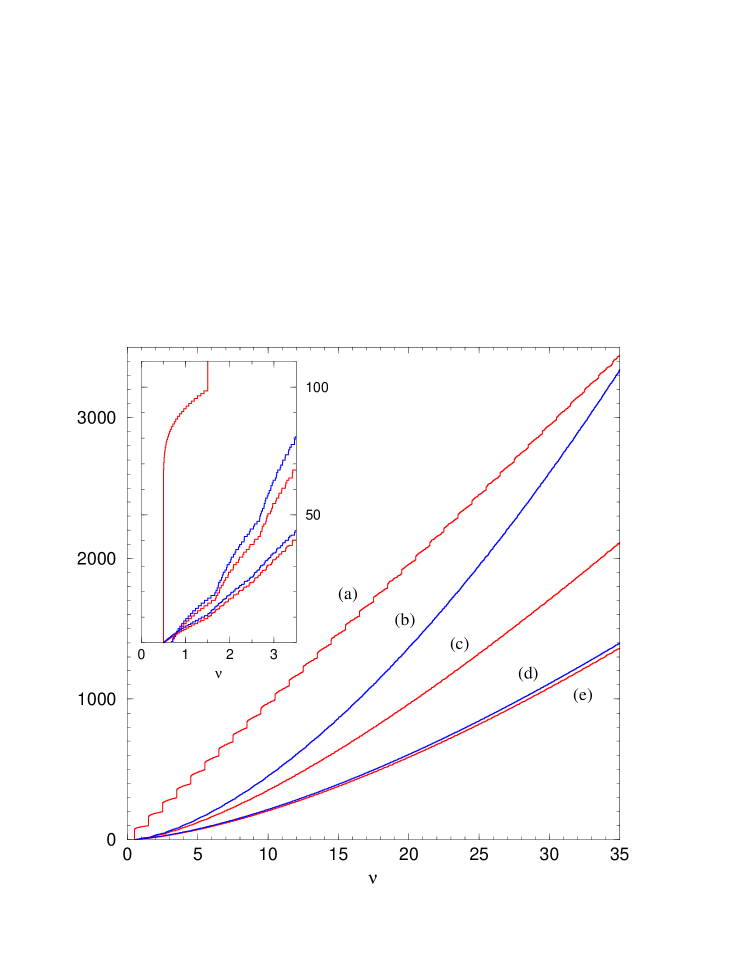
Figure 7.4: Spectral counting functions for the magnetic disk ($R/b=10$). (a) Total number of interior states. (b,c) Number of (b) exterior and (c) interior skipping states according to the angular momentum criterion. (d,e) Weighted number of edge states for the (d) exterior and (e) interior problem. When averaged the curves are well reproduced by the smooth counting functions, (3.10), (3.17), (3.16), and (7.6), respectively (not shown). The inset gives the counting functions for the first four Landau levels. The small kinks seen in ${\rm N}_{\rm skip}$ and ${\rm N}_{\rm edge}$ are damped away at higher energies.

In Figure 7.4 we compare various spectral counting functions obtained from the magnetic disk spectra given in Fig. 7.1. Curve (a) shows the total number of states in the interior. It exhibits distinct steps at the energies of the Landau levels. In the exterior a total counting function does not exist but the angular momentum criterion (6.88) enables counting the exterior states of the skipping type, see curve (b). The corresponding number of interior skipping states is indicated by curve (c). As one expects these two counting functions hardly exhibit steps at the Landau levels but they show a different functional dependence (given by eqs (3.17), (3.16)). In contrast, the weighted exterior and interior edge state counting functions, curves (d) and (e), respectively, display the same mean values to leading order. Their average is reproduced by eq (7.6) and no marks of the Landau levels are visible.

To examine more closely the suppression of the bulk states we plot the fluctuating part of the edge state counting function,

$${\rm N}^{\rm osc}_{\rm edge}(\nu)={{\rm N}}_{\rm edge}(\nu)-\overline{{\rm N}}_{\rm edge}(\nu)\ .$$ (7.7)

Figure 7.5 shows this quantity as obtained from the exterior spectrum. One observes that the fluctuating function hardly exhibits a signature of the Landau levels. The dotted line depicts ${\rm N}^{\rm osc}_{\rm edge}(\nu)$ after convolution with a narrow Gaussian which smoothes out the fluctuations. Its oscillations are due to the remnant contributions of the bulk states which are slowly damped out for higher energies. The fluctuating part of the exterior ellipse spectrum shown in Fig. 7.3 looks very similar [106].

\psfrag{y}{${{\rm N}}_{\rm edge}^{\rm osc}(\nu)$}\psfrag{xn}{$\nu$}\includegraphics[width=390.25534pt]{figs/Neflucdisk.eps}

Figure 7.5: Solid line: Oscillatory part (7.7) of the edge state counting function for the exterior magnetic disk ($R/b=10$). (The unspecified constant part of $\overline{{\rm N}}_{\rm edge}$ was not subtracted.) Dotted line: The oscillatory part convoluted by a Gaussian of width $\sigma=0.1$ minus an offset of $3.0$.

7.2.2 The semiclassical density of edge states

The standard spectral density (3.9) is given by the derivative of the number counting function ${\rm N}(\nu)$ with respect to energy. The edge state density (7.1) may also be formally defined as a derivative, now with respect to the boundary mixing parameter $\Lambda$, at Dirichlet boundary conditions ($\Lambda=0$),

$$d_{\rm edge}(\nu)=-\left.\frac{\mathrm{d}{\rm N}(\nu)}{\mathrm{d}\Lambda}\right|_{\Lambda=0}\equiv\,-\frac{b}{2\sqrt{\nu}}\,\left.\frac{\mathrm{d}{\rm N}(\nu)}{\mathrm{d}\lambda}\right|_{\lambda=0}\ .$$ (7.8)

Hence, the periodic orbit expression for the oscillatory part of the edge state density can be deduced immediately once we have the semiclassical formula for ${{\rm N}}_{\rm osc}$ at hand. For the time being, we restrict ourselves to hyperbolic systems. Combining the results of the previous chapter (eqs (6.54), (6.112a), and (6.113)), the number of states based on the skipping part of phase space is given by

$${\rm N}_{\rm osc}^{\rm skip}(\nu;\Lambda)=\frac{1}{\pi}\sum_{{\gamma}} \frac{(-)^{n_{\gamma}}}{r_{\gamma}\,\big{|}\mathop{\mathrm{tr}}\nolimits{\rm M}({\gamma})-2\big{|}^{\frac{1}{2}}}\,$$ (7.9)

$$\times \sin\Big{(}2\pi\nu{\rm A}({\gamma})-\frac{\pi}{2}\mu_{\gamma}-2\Lambda\sum_{j=1}^{n_{\gamma}}|\hat{\mathbf{n}}_{j}\hat{\mathbf{v}}_{j}|\Big{)}\ +\mathord{\mathrm{O}}(\Lambda^{2})\ .$$

Compared to (6.54) the leading order dependence on $\Lambda$ is included, as discussed in Sect. 6.5.3. (See Tables 6.1 and 6.2 for the definition of the various quantities in (7.9).) Since the semiclassical bulk states do not depend on the boundary condition their contribution vanishes when taking the derivative. Using (7.8) one obtains the semiclassical trace formula for the edge state density at Dirichlet boundary conditions,

$$d_{\rm edge}^{\rm osc}(\nu)=\frac{2}{\pi}\sum_{\gamma}\frac{\sum_{j=1}^{n_{\gamma}}|\hat{\mathbf{n}}_{j}\hat{\mathbf{v}}_{j}|}{r_{\gamma}\,\big{|}\mathop{\mathrm{tr}}\nolimits{\rm M}({\gamma})-2\big{|}^{\frac{1}{2}}}\cos\Big{(}2\pi\nu{\rm A}({\gamma})-\pi n_{\gamma}-\frac{\pi}{2}\mu_{\gamma}\Big{)}\ .$$ (7.10)

This expression should be compared to that of the unweighted density of states (6.61) which was obtained by taking the derivative with respect to the energy $\nu$. It exhibits the scaled time of flight $\tau_{\gamma}$ (6.60) in the numerator. Hence, the periodic orbit sum (7.10) differs from the standard spectral density only by the prefactors

$$w_{\gamma}:=\frac{\sum_{j=1}^{n_{\gamma}}|\hat{\mathbf{n}}_{j}\hat{\mathbf{v}}_{j}|}{\tau_{\gamma}}\ .$$ (7.11)

They attribute an individual classical weight to each skipping periodic orbit ${\gamma}$. The classical weights are given by the time averaged value for the normal component of the velocity $|\hat{\mathbf{n}}\,\hat{\mathbf{v}}|$ at the points of reflection. They vanish for cyclotron orbits. Similar to the quantum weights, the $w_{\gamma}$ lead to a gradual transition from edge to bulk contributions. It is easy to see that in the limit of a “grazing” trajectory of increasingly many short arcs variations in the curvature of the boundary may be neglected and the classical weights $w_{\gamma}$ approach a constant value. In the opposite case of an orbit which is almost detached from the boundary the weights vanish since the normal components of the velocities approach zero at a finite time of flight in the denominator of (7.11).

It is instructive to compare the distributions of quantum and classical weights. A direct comparison is not possible since the classical and the quantum weights are associated with different objects, eigenvalues and periodic orbits, respectively. In Fig. 7.6 we compare the distribution of classical weights to the corresponding weighted quantum spectrum. The data were obtained for the interior elliptic billiard, and are given in both cases as a function of the classical cyclotron radius $\rho$. The shade in the distribution of classical weights gives the probability for obtaining a certain weight if the trajectories are chosen randomly with respect to the invariant measure. It was approximated numerically by the histogram over a finite number of trajectories taken uniformly from phase space. Remarkably, one observes that the characteristic features of both distributions coincide. This shows that the quantum weights may be considered the expectation values of an observable which has a classical limit, ie, they measure a classical property. This holds in spite of the fact that the $w_{n}$ are defined in terms of the boundary condition, which has no classical analogue.

The bifurcating structures seen in Fig. 7.6 are due to stable periodic orbits. At the bifurcation points periodic orbits ${\smash{\gamma^{(n)}}}$ with a fixed number of reflections $n_{\gamma}$ exhibit the smallest possible cyclotron radius ($n_{\gamma}=6$ in the case of the rightmost structure). As the cyclotron radius increases, the orbits turn into pairs with either longer or shorter arcs. (Some of the corresponding islands of stability in phase may be identified in Fig. 3.1, left column.)

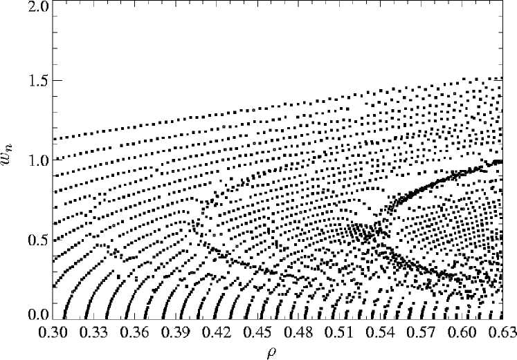
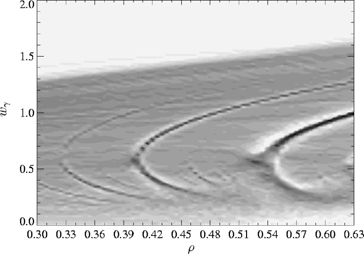
Figure 7.6: Weighted edge spectrum (7.1) (top) and phase space distribution of the classical weights (7.11) (bottom) for the interior ellipse. To ease comparison, also the quantum spectrum (calculated at constant $b=0.1$, as in Fig. 7.3) is given in terms of the classical cyclotron radius ( $\rho=b\times\sqrt{\nu}$.) One observes that the quantum weights tend to mimic the structures in the distribution of classical weights (which are due to stable islands in phase space, cf Fig. 3.1). [figure quality reduced]

7.3 Asymptotic properties of edge and bulk states

We proceed to briefly discuss the leading order behavior of the bulk energies and the smooth part of the edge counting function. Both estimates are obtained in the semiclassical limit such that it is legitimate to substitute the boundary by the straight line with periodic boundary conditions discussed in Appendix A.6. The finite mean curvature and variations of the boundary curvature are expected to appear only as higher order corrections, see the discussion in Sect. 3.3.3.

7.3.1 Bulk state energies and weights

\psfrag{deltanum}{$\Delta\nu_{m}$}\psfrag{wm}{$w_{m}$}\includegraphics[width=346.89731pt]{figs/LLdisk.eps}

Figure 7.7: Bulk state energy shifts $\Delta\nu_{n}$, and weights $w_{n}$, for the magnetic disk ($R/b=15.0111$) at the 50th Landau level (on a double-logarithmic scale). The interior ($\bullet\,$) and exterior ($\circ\,$) bulks states are approximated by the periodic line ($\boldsymbol{\times}$), cf (7.12) and (7.13).

The energy shift of a bulk state for general boundary condition is derived in Appendix A.6 by a uniform approximation, see (A.51). An asymptotic expansion, which amounts to the WKB approximation in the energetically forbidden region, yields the expression

$$\Delta\nu_{m} \simeq\frac{1}{2\pi}\exp\Big{(}-2\nu\big{(}q_{m}\sqrt{q_{m}^{2}-1}-\log\big{(}q_{m}+\sqrt{q_{m}^{2}-1}\big{)}\big{)}\Big{)}$$ (7.12)

$$\sim\frac{1}{2\pi}\,\bigg{(}\frac{2\pi bm}{\mathrsfs{L}({N+{\frac{1}{2}}})^{\frac{1}{2}}}\bigg{)}^{2N+1}\!\!\exp\Big{(}{N+{\frac{1}{2}}-2\Big{(}\frac{\pi bm}{\mathrsfs{L}}\Big{)}^{2}}\Big{)}\quad\text{as $m\to\infty$\ ,}$$ (7.12a)

with $N\in{{\mathbb{N}}}$ the Landau level and $q_{m}$ the quantized distance of the cyclotron center to the boundary, as defined in (A.49). We observe that the bulk state energies approach the Landau levels exponentially fast (indeed, like a Gaussian) as the integer $m$ increases, ie, as the distance of the cyclotron motion from the boundary grows.

The weights of bulk states follow likewise, by taking the derivative of equation (A.51). Essentially, they decay as fast as the shifts of the bulk energies:

$$w_{m}\simeq 2\,\bigg{(}\frac{\pi^{2}b^{2}m^{2}}{\mathrsfs{L}^{2}(N+{\frac{1}{2}})}-1\bigg{)}^{\frac{1}{2}}\Delta\nu_{m}$$ (7.13)

In Figure 7.7 we show exact bulk state energies and weights in a double-logarithmic representation. They belong to the interior and the exterior disk at $R/b=15.0111$ and to the 50th Landau level. The crosses indicate the zero curvature estimates according to eqs (7.12) and (7.13). One observes that the asymptotic weights and the spacing between the asymptotic energies match approximately the exact values, and lie between those of the finite curvature case. The approximation is improved when both $m$ and $N$ increase.

7.3.2 The mean edge counting function

As a second application, the periodic straight line problem allows the straightforward derivation of the leading term of the mean edge state counting function (7.6). We simply identify the transverse quantum number $n$ as a partial counting function for states with fixed quantum number $m$. An explicit formula for $n$, which includes the dependence on $\Lambda$ follows from $\smash{\xi_{\rm line}^{\rm(sc)}}=0$ (A.6.1). The sum

$${\rm N}_{\rm skip}(\nu,\Lambda)=\sum_{m}n(m,\Lambda)$$ (7.14)

yields the total number of states corresponding to skipping motion. Taking the derivative with respect to $\Lambda$ and replacing the summation by an integral we obtain the leading order of the smooth edge state density,

$$\overline{d}_{\rm edge}(\nu) =\left.-\frac{\mathrm{d}\overline{{\rm N}}_{\rm skip}(\nu;\Lambda)}{\mathrm{d}\Lambda}\right|_{\Lambda=0}=\frac{1}{\pi}\int_{-\sqrt{\nu}}^{\sqrt{\nu}}\Big{(}{1-\frac{{\tilde{c}_{y}}^{2}}{\nu}}\Big{)}^{\frac{1}{2}}\,\frac{\mathrsfs{L}\,\mathrm{d}\tilde{c}_{y}}{\pi b}\ +\mathord{\mathrm{O}}(1)$$

$$=\frac{\mathrsfs{L}}{2\pi b}\sqrt{\nu}\ +\mathord{\mathrm{O}}(1)\ .$$ (7.15)

The same result can be derived from the magnetic disk problem discussed in Sect. 6.5.2. It follows from (6.97) that the semiclassical spectrum is obtained by requiring that the phase

$$\varphi^{\rm int/ext}_{m}(\nu,{\widetilde{R}},\Lambda)=\Phi^{\rm int/ext}_{\rm disk}(\nu,m,{\widetilde{R}})\mp\alpha_{\Lambda}(\nu,m,{\widetilde{R}})-\frac{\pi}{4}$$ (7.16)

is an integer multiple of $\pi$. Hence, the smooth counting function of the skipping states is obtained by

$$\overline{{\rm N}}^{\rm int/ext}_{\rm skip}(\nu,{\widetilde{R}},\Lambda)=\frac{1}{\pi}\sum_{m}\varphi^{\rm int/ext}_{m}(\nu,{\widetilde{R}},\Lambda)\ ,$$ (7.17)

where the sum can be replaced by an integral over the interval $|m-{\widetilde{R}}^{2}|<2\nu^{\frac{1}{2}}{\widetilde{R}}$. Using the (6.96) one gets

$$\overline{d}_{\rm edge}(\nu) =\left.-\frac{\mathrm{d}\overline{{\rm N}}^{\rm int/ext}_{\rm skip}}{\mathrm{d}\Lambda}\right|_{\Lambda=0}\simeq\nu^{\frac{1}{2}}{\widetilde{R}}=\frac{\mathrsfs{L}}{2\pi b}\nu^{\frac{1}{2}}$$ (7.18)

which reproduces (7.3.2). This is further evidence that the periodic line problem yields the leading order terms consistently. The second order term in (7.4) is not obtained this way. It will be deduced in the next section by relating the quantum weights of the disk to the magnetic moments of the states.

7.4 Edge magnetization as a spectral measure

The preceeding section showed that our first definition (7.3) of the quantum weights yields an efficient and mathematically natural way to separate edge from bulk. However, the physical interpretation of the mixed boundary conditions is not immediate [76]. We therefore propose an alternative definition of the weights which is physically more accessible. It is obtained from the expectation value of the magnetic moment of the state.

In Section 3.4 we introduced the edge magnetization (3.28) of an interior billiard. It gives the scaled excess magnetization that is induced by the presence of the billiard boundary and was defined as

$$\widetilde{\mathcal{M}}_{\rm edge}(\nu) =\sum_{n=1}^{\infty}b^{2}\frac{\mathrm{d}\nu_{n}}{\mathrm{d}b^{2}}\,\Theta(\nu-\nu_{n})\ .$$ (7.19)

Like the edge state counting function (7.5) this is a weighted staircase. The size of the steps are now given by a derivative with respect to the magnetic length rather than $\Lambda$. Since the Landau levels do not depend on $b$ the bulk states contribute merely to a negligible degree to (7.19), as discussed in Sect. 3.4. Hence, it is reasonable to extend the definition (7.19) of the edge magnetization to the exterior problem.

The exterior edge current shows an orientation which is opposite to the interior (see Sect. 5.2). Therefore, one expects $\widetilde{\mathcal{M}}_{\rm edge}$ to turn negative in the exterior – which is indeed found. Moreover, the mean is finite in both cases and given by

$$\overline{\mathcal{M}}_{\rm edge}(\nu) =\pm{\frac{1}{2}}\,\frac{\mathrsfs{A}}{b^{2}\pi}\nu^{2}-\frac{1}{3}\,\frac{\mathrsfs{L}}{2\pi b}\nu^{\frac{3}{2}}\ .$$ (7.20)

The interior case (upper sign) follows from eq (3.32) while the exterior one (lower sign) is suggested by symmetry and confirmed empirically. Like in the case of the edge counting function (7.5) the moduli of the mean interior and exterior edge magnetizations are equal to leading order. This suggests to use the edge magnetization density

$$\widetilde{{\rm m}}_{\rm edge}(\nu)=\frac{\mathrm{d}}{\mathrm{d}\nu}\,\mathcal{M}_{\rm edge}(\nu)=\sum_{n=1}^{\infty}b^{2}\,\frac{\mathrm{d}\nu_{n}}{\mathrm{d}b^{2}}\,\delta(\nu-\nu_{n})\ ,$$ (7.21)

which was introduced in Sect. 3.4, to define a physically motivated spectral measure for the edge states:

$$d_{\rm edge}^{\scriptscriptstyle(\mathcal{M})}(\nu):=\pm\frac{1}{\nu}\,\widetilde{{\rm m}}_{\rm edge}(\nu)=\sum_{n=1}^{\infty}w_{n}^{\scriptscriptstyle(\mathcal{M})}\,\delta(\nu-\nu_{n})$$ (7.22)

The index ${\scriptstyle(\mathcal{M})}$ is used to distinguish this magnetization based density of edge states from the former definition (7.3). The weights are now given by

$$w_{n}^{\scriptscriptstyle(\mathcal{M})}:=\pm\frac{b^{2}}{\nu}\frac{\mathrm{d}\nu_{n}}{\mathrm{d}b^{2}}=\pm\frac{\langle\psi_{n}|{\frac{\tilde{\mathbf{r}}\times\tilde{\mathbf{v}}}{2}}|\psi_{n}\rangle+\nu}{\nu}\ .$$ (7.23)

Again, these positive quantities may be obtained as derivatives of the energies with respect to an external parameter (which is the magnetic length $b$ in the present case). At the same time they are expressed in terms of the (symmetrized) expectation values of the scaled magnetic moment (3.25). The weights vanish as the Landau levels are approached since for interior and exterior bulk states the scaled magnetic moment approaches the diamagnetic value $\langle\psi_{n}|{\frac{\tilde{\mathbf{r}}\times\tilde{\mathbf{v}}}{2}}|\psi_{n}\rangle\to-\nu$ from above and below, respectively. As for the smooth edge state density, the expression is obtained immediately from (7.20):

$$\overline{d}_{\rm edge}^{\scriptscriptstyle(\mathcal{M})}(\nu)=\pm\frac{1}{\nu}\frac{\mathrm{d}\overline{\mathcal{M}}_{\rm edge}}{\mathrm{d}\nu}=\frac{\mathrsfs{A}}{b^{2}\pi}\mp{\frac{1}{2}}\frac{\mathrsfs{L}}{2\pi b}\nu^{-{\frac{1}{2}}}$$ (7.24)

It coincides with the standard mean density for the interior case. Moreover, the interior weights approach unity as the magnetic field $B$ is decreased and bulk states no longer exist in the interior. This is seen immediately if we write the weight (7.23) in terms of conventional units

$$w_{n}^{\scriptscriptstyle(\mathcal{M})}=\pm\left(\frac{q\,B}{2E}\langle\psi_{n}|\mathbf{r}\times\mathbf{v}|\psi_{n}\rangle+1\right)\ .$$ (7.25)

In the limit $B\to 0$ the interior weights assume unit value and the interior edge state density turns into the standard density. This limit does not make sense in the exterior since in this case the spectrum ceases to be discrete; at finite field the exterior weights remain always non-negative.

The expression (7.25) shows that the weighted spectrum may be obtained immediately by measuring the magnetic moments of the states. The scaled magnetization density 3.26 follows from the conventional magnetization density (3.21) by a simple multiplication with the magnetic field:

$$\widetilde{{\rm m}}(\nu,b^{2})=B\,{\rm m}\big{(}E=\frac{2\hbar^{2}}{m_{e}b^{2}},B=\frac{2\hbar}{qb^{2}}\big{)}$$ (7.26)

This relation to an experimentally measurable quantity is a clear advantage of the present definition of the edge state density. It is achieved at a price — the leading order of the mean edge density is now determined by the area of the billiard rather than by its circumference, see (7.24). It indicates that with this measure the quasi one-dimensional character of the edge states is not accounted for to the same degree as by the former definition of $d_{\rm edge}$. However, it does an equally good job in consistently suppressing the bulk contributions. Moreover, in the case of a disk both spectral densities, $d_{\rm edge}$ and $d_{\rm edge}^{\scriptscriptstyle(\mathcal{M})}$, are identical up to a factor. This is seen from (A.27) which leads to the equation

$$w^{\scriptscriptstyle(\mathcal{M})}_{n}=w_{n}\,\frac{R}{b}\,\nu^{-{\frac{1}{2}}}\ .$$ (7.27)

This relation is as surprising as fortuitous and does not hold for general billiard shapes. Nonetheless, it allows to deduce the second, constant term of the mean density (7.4) by comparison with the smooth edge state density (7.24). Being the next order after the circumference term it is determined by the mean curvature which is equal for all simply connected boundaries, $\int_{\Gamma}\kappa(s)\mathrm{d}s=$ $\pm 2\pi$ (according to the Gauss-Bonnet theorem).

It follows from (7.27) that for the disk the magnetization based edge spectra differ from the spectra shown in Fig. 7.1 merely by a geometric transformation and there is no need to reproduce them here. As for the ellipse, Figure 7.8 shows the weights as obtained from the edge magnetization. Like in Fig. 7.6 the structures in the distribution are reproduced by the probability density of the corresponding classical weights.

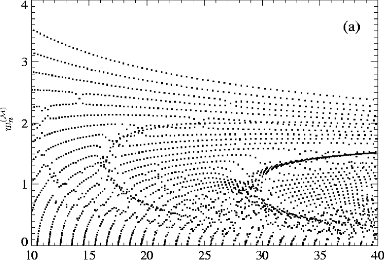
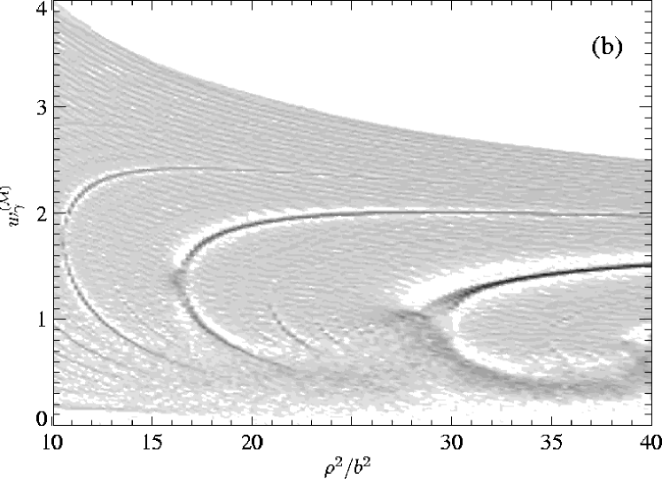
Figure 7.8: (a) Edge state spectrum using the edge magnetization weights (7.23) compared to (b) the phase space distribution of the classical weights (7.4) for the interior ellipse. [figure quality reduced]

Semiclassical edge magnetization

The semiclassical periodic orbit formula for the complete magnetization density is given in (6.63). Likewise, one finds that $\pm\widetilde{{\rm m}}^{\rm osc}_{\rm edge}/\nu$ has the form of the trace formula for the standard density with each periodic orbit now weighted individually by

$$w_{\gamma}^{\scriptscriptstyle(\mathcal{M})} :=\mp\,\frac{\displaystyle b^{2}\frac{\mathrm{d}}{\mathrm{d}b^{2}}\big{[}2\pi\nu{\rm A}({\gamma})\big{]}}{\displaystyle\nu\frac{\mathrm{d}}{\mathrm{d}\nu}\big{[}2\pi\nu{\rm A}({\gamma})\big{]}}=\pm\,\frac{\displaystyle\sum\nolimits_{j=1}^{n_{\gamma}}\Big{(}-\sigma_{j}\sqrt{1-\sigma_{j}^{2}}-\frac{\mathbf{r}_{j+1}\times\mathbf{r}_{j}}{2\rho^{2}}\Big{)}}{\displaystyle\sum\nolimits_{j=1}^{n_{\gamma}}\Big{(}\frac{\pi}{2}+\arcsin(\sigma_{j})\Big{)}}$$

$$=\frac{2\mathrsfs{A}_{\gamma}\pm\rho\mathrsfs{L}_{\gamma}}{\rho\mathrsfs{L}_{\gamma}}\ ,$$ (7.28)

see (6.58a) and (6.62). Like in the case of $w_{\gamma}$, the classical weights $w^{\scriptscriptstyle(\mathcal{M})}_{\gamma}$ vanish as trajectories get almost detached from the boundary (since the numerator approaches $2\mathrsfs{A}$, while $\mathrsfs{L}_{\gamma}\to\infty$).

Equipped with well-defined spectral densities for edge states and the corresponding trace formulas we can now proceed with a statistical and semiclassical study of edge state spectra. We shall not only consider the statistics within a given edge state spectrum (in Chapter 8) but look also for cross correlations between different, classically related spectra (in Chapter 9).

8 Properties of edge state spectra

We apply the weighted spectral densities discussed in the previous chapter to analyze two aspects of the interior and the exterior edge spectra. First we perform a statistical analysis comparing the results to the predictions of random matrix theory. Second, we check the validity of the semiclassical trace formula taking the disk billiard as an example.

8.1 Universal auto-correlations

One of the central goals in the field of quantum chaos is to understand how the statistical properties of the quantum spectrum reflect the nature of the underlying classical dynamics [5]. We extend these studies to magnetic billiards by making use of the spectral measure of edge states introduced in the previous chapter. It was constructed to focus on the non-trivial part of phase space which is determined by the billiard boundary map (3.4).

As a first point we check whether the edge spectra of both interior and exterior magnetic billiards display the universal characteristics of random matrix theory (RMT) if the corresponding skipping motion is hyperbolic. Our quantity of choice to characterize the spectrum statistically is the spectral form factor $K(\tau)$. It is sensitive to correlations of the eigenenergies beyond the mean level spacing [107]. The standard form factor was already used in Chapter 5 to study the two-point correlations in the unweighted spectra of interior billiards. For edge spectra $K(\tau)$ is readily defined in terms of the 2-point autocorrelation function of the edge density,

$$R_{\nu_{0}}(\nu)=\int d_{\rm edge}^{\rm osc}\Big{(}\nu^{\prime}+\frac{\nu}{2}\Big{)}\,d_{\rm edge}^{\rm osc}\Big{(}\nu^{\prime}-\frac{\nu}{2}\Big{)}\,g_{1}(\nu^{\prime}-\nu_{0})\,\mathrm{d}\nu^{\prime}\ .$$ (8.1)

Here, we included a normalized Gaussian window function $g_{1}$ to pick up a spectral interval centered at $\nu_{0}$.

Before comparing to RMT it is advantageous to remove the trivially system-dependent properties of the spectrum by “unfolding” it [107]. This is a transformation of the spectrum which renders it dimensionless and of unit mean density. Dealing with a weighted spectrum the unfolding procedure must transform both the energies and the weights. The natural choice involves the smooth edge state counting function $\overline{{\rm N}}_{\rm edge}$ and the average weight $\langle w^{2}\rangle/\langle w\rangle$ in the spectral interval considered:

$$\check{\nu}_{n}:=\frac{\langle w\rangle}{\langle w^{2}\rangle}\,\overline{{\rm N}}_{\rm edge}(\nu_{n})\qquad\text{and}\qquad\check{w}_{n}:=\frac{\langle w\rangle}{\langle w^{2}\rangle}\,w_{n}\ .$$ (8.2)

Here, the first and second moments of the weights,

$$\langle w\rangle =\sum_{n=1}^{\infty}w_{n}\;g(\overline{{\rm N}}_{\rm edge}(\nu_{n})-\check{\nu}_{0})$$ (8.3)

and

$$\langle w^{2}\rangle =\sum_{n=1}^{\infty}w_{n}^{2}\;g(\overline{{\rm N}}_{\rm edge}(\nu_{n})-\check{\nu}_{0})\ ,$$ (8.4)

are taken locally in the spectrum in terms of the window function $g$ (a normalized Gaussian of width $\sigma_{g}$.) As a result of this unfolding, both the weights and the weighted density have unit mean.

Since we are dealing with a discrete spectrum, the form factor must be averaged to be well-defined. The standard procedure is to take the spectral average over non-overlapping parts of the spectrum,

$$K(\tau)=\left\langle\int\e^{2\pi\mathrm{i}\check{\nu}\tau}R_{\check{\nu}_{0}}(\check{\nu})\,g_{2}(\check{\nu})\,\mathrm{d}\check{\nu}\right\rangle_{\check{\nu}_{0}}$$ (8.5)

as indicated by the triangular brackets. According to the spectral ergodicity hypothesis [129] this should be equivalent to an ensemble average for hyperbolic systems.

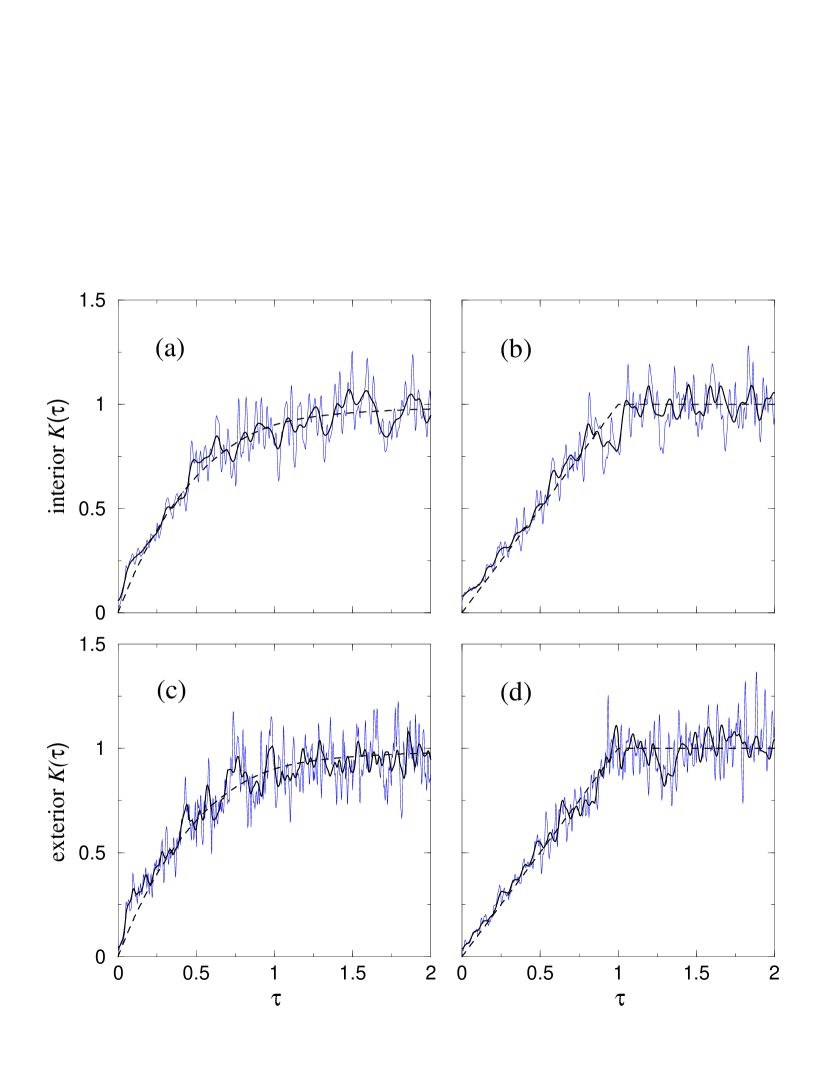
Figure 8.1: Form factors (8.6) of the interior (a,b) and exterior (c,d) edge state spectra for the asymmetric stadium (a,c) and skittle (b,d) billiard at $\rho=1.2$. The shapes are defined in Fig. 5.1. The functions follow the RMT predictions of the GOE and GUE ensembles [107], respectively (dashed lines). The heavy lines correspond to stronger spectral averaging than the thin lines ($\sigma_{g}=10$ and $\sigma_{g}=3$, respectively.)

If we choose the widths of the Gaussians $g_{1}$ and $g_{2}$ as $\sigma_{g}/\sqrt{2}$ and $\sigma_{g}\sqrt{2}$, respectively, the Fourier transform of the autocorrelation function leads directly to the power spectrum. The form factor is then given by the weighted sum

$$K(\tau)=\left\langle\frac{2\sqrt{2\pi}\sigma}{\langle w^{2}\rangle}\left|\sum_{n=1}^{\infty}\check{w}_{n}\,\mathrm{e}^{2\pi\mathrm{i}(\check{\nu}_{n}-\check{\nu}_{0})\tau}g(\check{\nu}_{n}-\check{\nu}_{0})-\hat{g}(\tau)\right|^{2}\right\rangle_{\check{\nu}_{0}}\ ,$$ (8.6)

where the Fourier transform of $g$ is denoted by $\hat{g}$.

The previous discussion holds for both definitions, (7.3) and (7.23), of the spectral density of edge states. However, it is necessary to keep the type of the underlying classical motion unchanged during the spectral averaging. This is conveniently done by taking the spectrum in the semiclassical rather than the conventional direction, see Sects. 2.3 and 3.3.2. In this case the quantum weights $w_{n}$ are simply obtained by taking the derivatives with respect to $\Lambda$ at fixed $\rho$, see Appendix A.7. In the present section we use only this first definition of a spectral density of edge states since it is not possible to define magnetization-based weights for the semiclassical direction.

\psfrag{x}{$w$}\psfrag{y}{$p(w)$}\includegraphics[width=346.89731pt]{figs/histoweights.eps}

Figure 8.2: Distribution of the quantum weights $w_{n}>0.1$ of the interior (shaded) and exterior (transparent) skittle spectrum at $\rho=1.2$. The histograms show peaks whose positions are well reproduced by the phase space estimates (8.7) and (8.8) (indicated by the arrows). Unlike the interior case, the exterior distribution shows a tail due to the transitional states which ranges to the small weights. (For normalization (bulk) states with weights smaller than $0.1$ had to be disregarded.)

Figure 8.1 shows the form factors for the interior (top) and exterior (bottom) edge state spectra for the asymmetric stadium (left) and skittle (right) billiard, respectively. The spectra were obtained in the semiclassical direction, at fixed $\rho=1.2$, ie, for the same situation as in Fig. 5.4. The weights were obtained by numerical differentiation with respect to $\Lambda$. We observe that the interior form factors follow the RMT prediction of the Gaussian Orthogonal and Gaussian Unitary Ensembles, respectively, as expected from the specific symmetry properties of the Hamiltonians. In the interior case this is not surprising. To ensure essential hyperbolicity of the classical motion the value of $\rho$ had to be chosen large such that the interior phase space consists only of skipping trajectories which cover it ergodicly. As a consequence, one expects that all interior states are edge states to an equal degree. Indeed, the interior weights are distributed narrowly around a mean value $\overline{w}$, given by the ratio of weighted and unweighted mean densities,

$$\overline{w}=\frac{\overline{d}_{\rm edge}^{(\rho)}(\nu)}{\overline{d}_{\rm tot}^{(\rho)}(\nu)}=\frac{\mathrsfs{L}\rho}{4\mathrsfs{A}}\ ,$$ (8.7)

as can be observed from the shaded histogram in Fig. 8.2. The weights do not provide additional information in this case, which explains why $K(\tau)$ reproduces the RMT prediction, like in the unweighted case.

In contrast, the standard form factor – like any other standard statistical function – does not even exist for the exterior spectrum, which is dominated by infinitely many bulk states. Nonetheless, we find that the exterior spectrum closely obeys the predictions of random matrix theory (bottom row of Fig. 5.4) if viewed in an appropriate way, ie, by means of the edge state density. This way, a crucial test for the consistency of the spectral measure of edge states is passed. The quantum weights succeed to filter out selectively the relevant edge states, which in turn exhibit the universal characteristics expected for chaotic motion.

The distribution of the exterior weights is given by the transparent histogram in Figure 8.2. One observes that the distribution of large weights is peaked like in the interior case. Again, the peak position is well described by the ratio of weighted and unweighted densities,

$$\overline{w}=\frac{\overline{d}_{\rm edge}^{(\rho)}(\nu)}{\overline{d}_{\rm skip}^{(\rho)}(\nu)}\simeq\frac{\mathrsfs{L}\rho}{2\mathrsfs{A}_{\rm skip}^{\rm ext}(\rho)}\ ,$$ (8.8)

with the mean unweighted density now given by the phase space estimate (3.15) of skipping states. Unlike the interior case, the distribution has a tail of transitional states which ranges to the infinitely many bulk states with small weights.

\psfrag{t}{$t$}\psfrag{y1}{ $-|\widehat{d}^{\rm(\rho,sc)}_{\rm edge}\!(t)|\quad|\widehat{d}^{\rm(\rho)^{osc}}_{\rm edge}\!(t)|$}\psfrag{y2}{ $-|\widehat{d}^{\rm(\rho,sc)}_{\rm edge}\!(t)|\quad|\widehat{d}^{\rm(\rho)^{osc}}_{\rm edge}\!(t)|$}\includegraphics[width=433.62pt]{figs/accompext.eps}

Figure 8.3: Action spectrum of the exterior disk at $\rho=2R$. The positive values give the Fourier transform (8.10) of the exterior edge density (absolute values). The positions of the peaks are well reproduced by the trace formula (8.9) (negative values) – except for the small peaks at integer $t$ which are remnants of the bulk states. The peak heights match well in most cases; they are expected to fit better if a spectral interval larger than $\nu\in[0;48]$ is used.

\psfrag{y1}{\small$-|\widehat{d}^{\rm(\rho,sc)}_{\rm edge}\!(t)|\quad|\widehat{d}^{\rm(\rho)^{osc}}_{\rm edge}\!(t)|$}\psfrag{y2}{\small$-|\widehat{d}^{\rm(\rho,sc)}_{\rm edge}\!(t)|\quad|\widehat{d}^{\rm(\rho)^{osc}}_{\rm edge}\!(t)|$}\psfrag{y3}{\small$-|\widehat{d}^{\rm(\rho,sc)}_{\rm edge}\!(t)|\quad|\widehat{d}^{\rm(\rho)^{osc}}_{\rm edge}\!(t)|$}\psfrag{t}{$t$}\includegraphics[width=433.62pt]{figs/accompint.eps}

Figure 8.4: Action spectrum of the interior disk at a cyclotron radius $\rho=0.4\times R$ small enough to enable bulk states. The Fourier transform (8.10) of the interior edge density (positive values, $\nu\in[0;60]$) is well reproduced by the trace formula (negative values). Note that in the top part, which shows the remnant peaks of bulk contributions, the y-axis has a different scale.

8.2 The action spectrum

We turn from the statistical analysis of edge spectra to their semiclassical description. Here, the main purpose is to show that the trace formula for the edge state density – which rates each periodic orbit with a classical weight – succeeds in approximating the exact edge spectrum.

We choose the disk billiard for which an explicit periodic orbit formula is readily obtained from equation (6.111). For the exterior case and $\Gamma_{\!\rm d}=R/\rho<1$ we find, see (7.8),

$$d^{\rm osc}_{\rm edge}(\nu)= \left(\frac{2\nu}{\pi}\right)^{\frac{1}{2}}\sum_{N=2}^{\infty}\,\frac{2}{N^{1/2}}\sum_{\Delta\varphi\in\mathcal{P}_{\rm ext}^{N}}\Big{|}\sin\Big{(}\alpha-\frac{\Delta\varphi}{2}\Big{)}\Big{|}$$ (8.9)

$$\times\frac{\sin(\alpha)\cos(\alpha)-{\frac{1}{2}}\Gamma_{\!\rm d}^{2}\sin(\Delta\varphi)}{(\sin(\alpha)\cos(\alpha))^{\frac{1}{2}}}\cos\left(2\pi\nu N\,{\rm a}_{\rm L}(\Delta\varphi)+N\frac{\pi}{2}-\frac{\pi}{4}\right)\ ,$$

with $\alpha$ defined by equation (6.65). (The term $|\sin(\alpha-\frac{\Delta\varphi}{2})|$ corresponds to the normal component of the velocity, $|\hat{\mathbf{n}}\,\hat{\mathbf{v}}|$, in (7.10).) Moreover, the exact quantum spectrum of the disk is calculated relatively easily in terms of the roots of special functions, see App. A.3. We calculated spectral intervals large enough so that the Fourier transformation of the spectral densities,

$$\widehat{d}^{{\rm osc}}_{\rm edge}\!(t)=\int\mathrm{e}^{2\pi\mathrm{i}\nu t}d^{{\rm osc}}_{\rm edge}\!(\nu)\,h(\nu-\nu_{0})\,\mathrm{d}\nu\ ,$$ (8.10)

resolves the classical actions $t$ of the underlying periodic orbits. Here, the function $h$ is a suitable window centered on the midpoint $\nu_{0}$ of the spectral interval. This action spectrum may be readily compared to the semiclassical prediction based on (8.9).

Like in the previous section, it is convenient to take the spectrum in the semiclassical direction, at constant $\rho$. In Figure 8.3 we show the action spectrum for the exterior disk at a cyclotron radius $\rho=2R$ (positive values). The corresponding prediction of the trace formula (8.9) is given by the negative values. One observes that the peak positions match very well with the predictions of semiclassical theory. The only exception are the small peaks at integer actions which are not reproduced semiclassically. They are remnants of the infinite number of bulk states. The peak heights are well reproduced most of the time, except if two peaks overlap too strongly. These deviations are expected to fade as a larger spectral interval is used and the the widths of the peaks decrease. This is also seen in Figure 8.4 where we present the exact and semiclassical action spectra of the interior magnetic disk – based on a large spectral interval ($\nu\in[0;60]$ at $\rho=0.4\times R$). Here, the cyclotron radius was chosen small enough for bulk states to exist in the interior. One observes again that the latter are very efficiently suppressed in the action spectrum giving rise only to the small peaks at integer values (shown in the top part of Fig. 8.4). In the Fourier transform of the unweighted density, in contrast, the bulk states obliterate the edge contributions such that not a single action is resolved (not shown). Blaschke and Brack [71] analyzed semiclassically the spectrum for the unweighted interior problem. The contribution of the bulk states was estimated and added by hand resulting in an unsatisfactory agreement between the semiclassical and the quantum spectra.

In conclusion, we find that the the semiclassical trace formula succeeds in reproducing the quantum edge state density. It does so by weighting each periodic orbit contribution with a classical weight which vanishes for cyclotron orbits. This removes the bulk contributions analogous to – and consistent with – the quantum weights of the edge state density.

\psfrag{sqrt(5)/2}{$\displaystyle{\frac{1}{2}}\sqrt{5}$}\psfrag{1.0}{$1.0$}\includegraphics[width=390.25534pt]{figs/s14shape.eps}

Figure 8.5: Definition of the Bunimovich stadium used in Sect. 8.3 and Chapter 9.

8.3 Using the edge magnetization

Finally, let us demonstrate that the edge state density may as well be defined in terms of the magnetization as discussed in Section 7.4.

Choosing the Bunimovich stadium billiard (defined in Fig. 8.5) we calculated the interior and exterior magnetization spectrum in the high-energy direction, at $b=0.2$. The selected spectral interval $\nu\in[100;135]$ corresponds to large cyclotron radii $\rho\in[2;2.32]$ giving rise to essentially hyperbolic classical motion. Quantum mechanically, the problem exhibits one unitary and one anti-unitary symmetry (rotation by $\pi$ and reflection at one axis, respectively). Hence, the spectrum decomposes into two symmetry classes (a feature which will be used in the next chapter) while each class should obey the characteristics of the Gaussian Orthogonal Ensemble [107].

\psfrag{x}{$\nu_{n}$}\psfrag{yext}{exterior $w^{\scriptscriptstyle(\mathcal{M})}_{n}$}\psfrag{yint}{interior $w^{\scriptscriptstyle(\mathcal{M})}_{n}$}\includegraphics[width=390.25534pt]{figs/mweights_stadium.eps}

Figure 8.6: Weights as obtained from the edge magnetization for the stadium billiard at $b=0.2$ and high energy. Note that the values of the weights differ in the (top) and exterior (bottom) by a factor of about ten. Notwithstanding, the mean edge state densities are equal to leading order. The classical cyclotron radius which corresponds to this part of the spectrum is large, $\rho\in[2;2.32]$, giving rise to essentially hyperbolic classical motion.

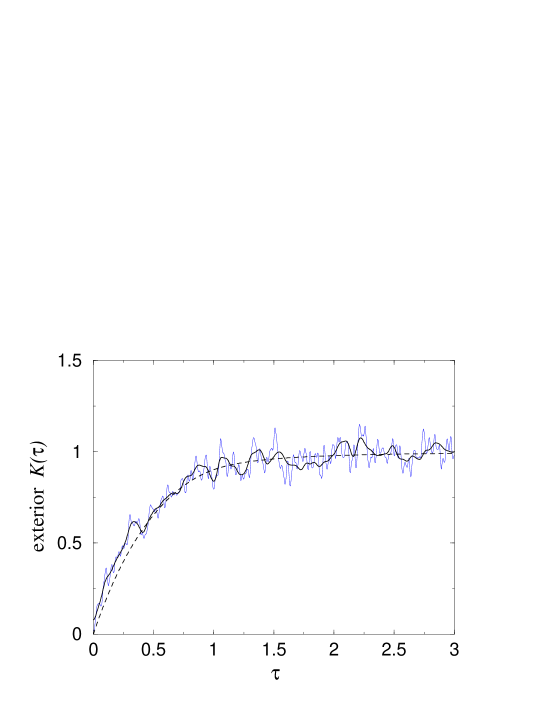
Figure 8.7: Form factor of the exterior Bunimovich stadium (Fig. 8.5) computed from the edge magnetization spectrum shown in Fig. 8.6, bottom part.

The weighted spectra are shown in Figure 8.6. Note that the weights are very different in magnitude, although they lead to the same average edge magnetization (7.20). This is explained by the different areas $\mathrsfs{A}_{\rm skip}$ of the interior and exterior skipping motion since the mean weight is asymptotically determined by the ratio

$$\overline{w}^{\scriptscriptstyle(\mathcal{M})}=\frac{\pm\overline{{\rm m}}_{\rm edge}(\nu)}{\nu\,\overline{d}_{\rm skip}(\nu)}\simeq\frac{\mathrsfs{A}}{\mathrsfs{A}_{\rm skip}(\rho=\sqrt{\nu}b)}\ ,$$ (8.11)

see (3.15) and (3.32); (in the interior case $\mathrsfs{A}_{\rm skip}=\mathrsfs{A}$). Similar to Fig. 8.2 the distributions of the magnetization weights are localized at $\overline{w}^{\scriptscriptstyle(\mathcal{M})}$ (not shown).

Figure 8.7 presents the form factor (8.5) of the exterior magnetization spectrum restricting the energies to a single symmetry class. As one expects the form factors follows the GOE prediction (dashed line). This indicates that the weights (7.23) based on the magnetization succeed to filter the bulk states consistently. They perform as well as the weights (7.3) based on the boundary condition.

9 Spectral cross correlations: The interior-exterior duality

The previous chapter focused on the correlations within a given interior or exterior edge spectrum and their relation to the corresponding classical dynamics. We now turn to a different type of question, namely, whether one can relate the interior and the exterior spectra belonging to the same billiard.

From a spectral theory point of view there is no apparent reason why the spectra of the magnetic Laplacian defined on complementary domains should have anything in common. However, it was shown in Section 3.2 that the classical periodic orbits of the interior and the exterior problem are in general intimately related. They come in dual pairs with equal stability and their actions adding up to an integer multiple of the action of a cyclotron orbit. Since the semiclassical spectra are determined by the sets of periodic orbits one expects that the correlation in the classical dynamics carries over to the quantum case inducing a relation between the interior and exterior spectra.

This observation being made it comes as a surprise that one does not find any signature of a cross-correlation if the spectra are analyzed with standard statistical methods, ie, the interior and exterior spectra of a billiard seem to be statistically independent (not shown). Nonetheless, it will be found in the present chapter that there exists indeed a strong cross-correlation between the two spectra. It can be observed only if a quantitative definition of edge states, as developed above, is at hand.

9.1 A semiclassical theory of spectral cross correlations

In order to unravel the connection between interior and exterior edge state energies a special cross-correlation function is needed. It not only involves the Dirichlet energies of the edge states but also relies crucially on the information provided by their weights.

The cross correlation function

As the first step to obtain the appropriate correlator, we formally extend the definition of the edge state density to finite boundary mixing parameters $\Lambda$.

$$d_{\rm edge}(\nu;\Lambda):=-\frac{\mathrm{d}}{\mathrm{d}\Lambda}{\rm N}(\nu;\Lambda)$$ (9.1)

The dependence of the spectral density on $\Lambda$ will be needed only in the vicinity of the Dirichlet boundary condition, $\Lambda=0$, (3.6), where an expansion to first order in $\Lambda$ is allowed. The spectral density (9.1) can then be written only in terms of the Dirichlet energies and Dirichlet weights,

$$d_{\rm edge}(\nu;\Lambda) =\sum_{n=1}^{\infty}\frac{\mathrm{d}\nu_{n}}{\mathrm{d}\Lambda}(\Lambda)\;\delta\big{(}\nu-\nu_{n}(\Lambda)\big{)}$$

$$\cong\sum_{n=1}^{\infty}\frac{\mathrm{d}\nu_{n}}{\mathrm{d}\Lambda}(0)\;\delta\Big{(}\nu-\nu_{n}(0)-\Lambda\,\frac{\mathrm{d}\nu_{n}}{\mathrm{d}\Lambda}(0)\Big{)}$$

$$=\sum_{n=1}^{\infty}\delta\Big{(}\frac{\nu-\nu_{n}}{w_{n}}-\Lambda\Big{)}\ ,$$ (9.2)

which follows from (7.3) and the properties of the $\delta$-function. The cross-correlation function is now defined as an integral over energy and boundary parameter

$$C(\nu_{0})=\int\!\!\!\int d^{\rm osc(int)}_{\rm edge}(\nu;\Lambda)\,d^{\rm osc(ext)}_{\rm edge}(\nu;-\Lambda)\,h(\Lambda)\,g(\nu-\nu_{0})\,\mathrm{d}\Lambda\,\mathrm{d}\nu\ ,$$ (9.3)

with normalized Gaussian window functions $h$ and $g$. Here, $h$ serves to restrict the integration over $\Lambda$ to the range where the linear approximation in (9.1) is valid and may have a width of order one. The function $g$ is needed to regularize the pair distribution $d^{\rm osc(int)}_{\rm edge}(\nu)\,d^{\rm osc(ext)}_{\rm edge}(\nu)$. It selects a narrow energy interval centered around the energy $\nu_{0}$ and should have the width of a few effective nearest neighbor spacings.

Inserting expression (9.1) the cross-correlation function turns into a double sum over the interior and exterior edge spectrum,

$$C(\nu_{0})=\sum_{i,j=1}^{\infty}\frac{w_{i}w_{j}^{\prime}}{w_{i}+w_{j}^{\prime}}\,g\!\left(\frac{\displaystyle\frac{\nu_{i}-\nu_{0}}{w_{i}}-\frac{\nu_{0}-\nu_{j}^{\prime}}{w_{j}^{\prime}}}{\displaystyle\frac{1}{w_{i}}+\frac{1}{w_{j}^{\prime}}}\right)h\!\left(\frac{\nu_{i}-\nu_{j}^{\prime}}{w_{i}+w_{j}^{\prime}}\right)-C_{\rm bg}\ ,$$ (9.4)

where the primes label the exterior energies and weights for the sake of brevity.

This pair correlation function is far from being standard since it relies heavily on the weights attributed to the individual levels. However, this function is the most natural choice to accentuate the spectral cross-correlations which originate from the underlying classical interior-exterior duality. This will be shown below. The important point to note is that due to the small width of $g$ only a few pairs of interior and exterior spectral points will contribute appreciably at a given $\nu_{0}$. It is the pairs with equal weighted distances from the left and right, respectively, to the reference energy $\nu_{0}$. Here, the energy differences are scaled individually by the reciprocal weight attached to each spectral point. The function $h$, in contrast, limits the absolute energy distance. Note also that the prefactor in (9.4) ensures that pairs which include at least one bulk state do not contribute appreciably to the sum.

The term $C_{\rm bg}$ in (9.4) subtracts the background. It is approximated by

$$C_{\rm bg}\cong\overline{d}_{\rm edge}(\nu_{0})\left(\sum_{i=1}^{\infty}h\Big{(}\frac{\nu_{i}-\nu_{0}}{w_{i}}\Big{)}+\sum_{j=1}^{\infty}h\Big{(}\frac{\nu_{j}^{\prime}-\nu_{0}}{w_{j}^{\prime}}\Big{)}-\overline{d}_{\rm edge}(\nu_{0})\right),$$ (9.5)

if we neglect the width of $g$ and disregard the fact that the interior and exterior mean edge densities differ in the higher order terms. We shall discuss the correlation function further after we derive its main properties using the semiclassical approximation.

The semiclassical correlator

We turn now to the semiclassical evaluation of the correlation function using the periodic orbit formula (7.2) discussed in Section 7.2.2. It applies to completely chaotic systems. One obtains a double sum over the skipping interior and exterior periodic orbits:

$$C(\nu_{0})=\int\!\!\mathrm{d}\nu\, g(\nu-\nu_{0})\,\,\frac{2}{\pi^{2}}\sum_{{\gamma},{\gamma}^{\prime}}\frac{w_{\gamma}\,\tau_{\gamma}}{r_{\gamma}\,|\mathop{\mathrm{tr}}\nolimits{\rm M}({\gamma})-2|^{\frac{1}{2}}}\,\frac{w_{{\gamma}^{\prime}}\,\tau_{{\gamma}^{\prime}}}{r_{{\gamma}^{\prime}}\,|\mathop{\mathrm{tr}}\nolimits{\rm M}({\gamma}^{\prime})-2|^{\frac{1}{2}}}\qquad\qquad$$

$$\times\Bigg{\{} \cos\left(2\pi\nu\big{(}{\rm A}({\gamma})+{\rm A}({\gamma}^{\prime})\big{)}-\pi(n_{\gamma}+n_{{\gamma}^{\prime}})-\frac{\pi}{2}(\mu_{\gamma}+\mu_{{\gamma}^{\prime}})\right)$$

$$\times\,\hat{h}\bigg{(}\frac{1}{\pi}\sum_{j=1}^{n_{\gamma}}|\hat{\mathbf{n}}_{j}\hat{\mathbf{v}}_{j}|-\frac{1}{\pi}\sum_{j=1}^{n_{{\gamma}^{\prime}}}|\hat{\mathbf{n}}_{j}^{\prime}\hat{\mathbf{v}}_{j}^{\prime}|\bigg{)}$$

$$+ \cos\left(2\pi\nu\big{(}{\rm A}({\gamma})-{\rm A}({\gamma}^{\prime})\big{)}-\pi(n_{\gamma}-n_{{\gamma}^{\prime}})-\frac{\pi}{2}(\mu_{\gamma}-\mu_{{\gamma}^{\prime}})\right)$$

$$\times\,\hat{h}\bigg{(}\frac{1}{\pi}\sum_{j=1}^{n_{\gamma}}|\hat{\mathbf{n}}_{j}\hat{\mathbf{v}}_{j}|+\frac{1}{\pi}\sum_{j=1}^{n_{{\gamma}^{\prime}}}|\hat{\mathbf{n}}_{j}^{\prime}\hat{\mathbf{v}}_{j}^{\prime}|\bigg{)}\Bigg{\}}$$ (9.6)

Here, $\hat{h}$ is the Fourier transform of the window function $h$, and the exterior quantities are again marked with a prime. The width of $\hat{h}$ is small compared to the sum over $|\hat{\mathbf{n}}_{j}\hat{\mathbf{v}}_{j}|$ (which is of order $n_{\gamma}$). As a result, the second term in the curly brackets of (9.1) is suppressed. In the first term of equation (9.1), $\hat{h}$ reduces the sum effectively to those pairs with approximately equal sums of angles of incidence $\sum_{j}|\hat{\mathbf{n}}_{j}\hat{\mathbf{v}}_{j}|=$ $\sum_{j}|\hat{\mathbf{n}}_{j}^{\prime}\hat{\mathbf{v}}_{j}^{\prime}|$. The dual pairs of periodic orbits discussed in Section 3.2.3 have precisely this property. Hence, the only systematic contribution to the correlator will come from these pairs. In Sect. 6.3.3 we discussed the relations between ${\gamma}$ and its dual partner orbit ${\overline{\gamma}}$, which may be summarized as

$$\begin{array}[]{rcl}{\rm A}({\gamma})+{\rm A}({\overline{\gamma}})&=&n_{\gamma}=n_{\overline{\gamma}}\ ,\\ \mathop{\mathrm{tr}}\nolimits{\rm M}({\overline{\gamma}})&=&\mathop{\mathrm{tr}}\nolimits{\rm M}({\gamma})\ ,\\ |{\hat{\mathbf{n}}}_{j}{\hat{\mathbf{v}}}_{j}|_{({\overline{\gamma}})}&=&|\hat{\mathbf{n}}_{j-n_{\gamma}}\hat{\mathbf{v}}_{j-n_{\gamma}}|_{({\gamma})}\ ,\end{array}\qquad\quad\begin{array}[]{rcl}r_{\overline{\gamma}}&=&r_{\gamma}\ ,\\ \mu_{\overline{\gamma}}&=&2n_{\gamma}-\mu_{\gamma}\ ,\\ w_{\overline{\gamma}}\,\tau_{\overline{\gamma}}&=&w_{\gamma}\,\tau_{\gamma}\ .\end{array}$$ (9.13)

If we retain only the contributions of the dual pairs the cross-correlation function simplifies to a single sum over interior (or exterior) periodic orbits. Assuming global classical duality we obtain

$$C(\nu_{0})=\frac{2}{\pi^{2}}\sum_{\gamma}\frac{w_{\gamma}^{2}\,\tau_{\gamma}^{2}}{r_{\gamma}^{2}\,|\mathop{\mathrm{tr}}\nolimits{\rm M}({\gamma})-2|}\cos(2\pi n_{\gamma}(\nu_{0}-\tfrac{1}{2}))\,\,\hat{g}(n_{\gamma})\ .$$ (9.14)

The restriction of the double sum (9.1) to the dual pairs is tantamount to the diagonal approximation used in the semiclassical evaluation of the autocorrelation function [108]. In the present case, the actions of the chosen pairs of periodic orbits complement each other to an integer $n_{\gamma}$, while in the usual diagonal approximation it is the resonant terms, ${\rm A}({\gamma})-{\rm A}({\gamma}^{\prime})=0$, which give the dominant “diagonal” contribution.

In deriving (9.14) the energy dependence of the amplitudes of the trace formula could be neglected since the variation of the energy was assumed to be small on the classical scale in (9.3). If $\nu_{0}$ is taken large (i.e. we are in the semiclassical regime of the spectrum) the classical quantities in (9.14) will hardly change as $\nu_{0}$ is varied. By grouping together the contributions from all the periodic orbits with the same number of reflections $n_{\gamma}$ we obtain

$$C(\nu_{0}) =\sum_{n=n_{\rm min}}^{\infty}f(n)\,\hat{g}(n)\,\cos(2\pi n(\nu_{0}-\tfrac{1}{2}))\ ,$$ (9.15)

with

$$\qquad f(n) =\frac{2}{\pi^{2}}\sum_{{\gamma}:n_{\gamma}=n}\frac{w_{\gamma}^{2}\,\tau_{\gamma}^{2}}{r_{\gamma}^{2}\,|\mathop{\mathrm{tr}}\nolimits{\rm M}({\gamma})-2|}\ .$$ (9.16)

Assuming ergodicity, the weighted sum over classical $n$-orbits (9.16) can be calculated as a phase space average. For large $n$ it takes on the universal value $f(n)=n/8$. At the same time, the number of reflections $n_{\gamma}$ is geometrically bounded from bellow, $n\geq n_{\rm min}$, for a given cyclotron radius. Hence,

$$f(n)=\begin{cases}0&\text{for $n<n_{\rm min}$}\\ \frac{1}{8}n&\text{as $n\gg n_{\rm min}$\ .}\end{cases}$$ (9.17)

Equation (9.15) makes a clear prediction on the form of the cross-correlation function. Even if the classical dynamics changes slowly as $\nu_{0}$ is varied the infinite sum (9.15) will be appreciable only at energies $\nu_{0}=N+\tfrac{1}{2}$, $N\in\mathbb{N}_{0}$, where the cosine terms are stationary. We therefore expect the cross-correlation function to display pronounced, equidistant peaks at large energies. Their positions are expected to coincide with the Landau levels (although they have nothing to do with bulk states) and their appearance provides a direct quantum manifestation of the existence of classically dual orbits.

If the billiard exhibits a discrete symmetry the semiclassical theory suggests also a natural way to test that the predicted structures in $C(\nu_{0})$ are not artefacts (eg due to the bulks states). In this case the cross correlation between exterior and interior spectra with different symmetries is derived in a similar fashion as (9.15). However, now we have

$$f(n)=\frac{2}{\pi^{2}}\sum_{{\gamma}:n_{\gamma}=n}(-)^{s_{\gamma}}\frac{w_{\gamma}^{2}\,\tau_{\gamma}^{2}}{r_{\gamma}^{2}\,|\mathop{\mathrm{tr}}\nolimits{\rm M}({\gamma})-2|}\ ,$$ (9.18)

where $s_{\gamma}$ counts the number of times the periodic orbit ${\gamma}$ crosses the symmetry line [130]. Since in the sum $s_{\gamma}$ will be even or odd with equal frequency the terms cancel on average and no correlation signal is expected.

Action cross correlations

Next, we consider the Fourier transform of the cross-correlation function (9.3) which highlights its fluctuating part. The semiclassical theory predicts a sequence of equidistant $\delta$-spikes at integer values,

$$D(t)=\int\!C(\nu_{0})\,\e^{-2\pi\mathrm{i}\nu_{0}t}\mathrm{d}\nu_{0}=\frac{1}{2}\sum_{n=n_{\rm min}}^{\infty}(-)^{n}f(n)\,\hat{g}(n)\,\delta(n-t)\ .$$ (9.19)

They correspond to the sums of the actions of dual pairs, which complement each other to integer values, starting from the minimal number of reflections $n_{\rm min}$.

Using the edge magnetization

Let us turn to the question whether the correlation is also seen if one uses the spectral density $d_{\rm edge}^{\scriptscriptstyle(\mathcal{M})}$ based on the edge magnetization (7.21) as the spectral measure. It has the advantage of being easier to measure both numerically and in experiments since one does not have to change the boundary conditions. The theoretical treatment is completely analogous to the above with the correlation function now involving an integration over the the magnetic length parameter $b$ rather than the boundary condition:

$$C_{\rm mag}(\nu_{0}) =\int\!\!\!\int d^{\rm osc{\scriptscriptstyle(\mathcal{M})}}_{\rm edge(int)}(\nu;b^{2})\,d^{\rm osc{\scriptscriptstyle(\mathcal{M})}}_{\rm edge(ext)}(\nu;b^{2})\;h\Big{(}\frac{b^{2}-b_{0}^{2}}{b_{0}^{2}}\Big{)}\,\frac{\mathrm{d}(b^{2})}{b_{0}^{2}}\,$$

$$\phantom{=\int\!\!\!\int}\times g(\nu-\nu_{0})\,\mathrm{d}\nu\ .$$ (9.20)

The linear expansion of the dependence of the energies on $b^{2}$ yields a double sum like eq (9.4) with the $w_{n}$ replaced by the magnetic weights $w_{n}^{\scriptscriptstyle(\mathcal{M})}$ (7.23). Semiclassically, the integration over $\delta b^{2}$ selects those pairs of interior and exterior orbits which satisfy

$$w^{\scriptscriptstyle(\mathcal{M})}_{\gamma}\,\tau_{\gamma} =w^{\scriptscriptstyle(\mathcal{M})}_{{\gamma}^{\prime}}\,\tau_{{\gamma}^{\prime}}\ ,$$ (9.21)

ie,

$$(\mathrsfs{L}_{\gamma}+\mathrsfs{L}_{\gamma}^{\prime})\rho =2(\mathrsfs{A}_{\gamma}+\mathrsfs{A}_{\gamma}^{\prime})\ ,$$ (9.21a)

which is again the dual pairs, ${\gamma}^{\prime}={\overline{\gamma}}$. (This may be seen from eqs (7.4) and (6.60) since the signs of the $\sigma_{j}$ (6.55) and the order of the points of reflection $\mathbf{r}_{j}$ are reversed as one goes from an orbit to its dual. Geometrically, it is evident that dual orbits with $N$ reflections satisfy $\mathrsfs{L}_{\gamma}+\mathrsfs{L}_{\overline{\gamma}}=2\pi\rho N$ and $\mathrsfs{A}_{\gamma}+\mathrsfs{A}_{\overline{\gamma}}=\rho^{2}\pi N$.)

These predictions for the cross-correlation function are not restricted to purely chaotic dynamics, although the bouncing map was assumed to be hyperbolic, so far. For the (integrable) disk one obtains a completely analogous result. The function $f(n)$ is not universal in this case, but the prediction remains that $C(\nu_{0})$ is peaked at the energies of the Landau levels. Below, in Sect. 9.3 it will be shown that semiclassical correlations can be predicted even for mixed chaotic systems (without resorting to periodic orbit theory).

9.2 Numerical evidence

In this section we provide numerical evidence supporting the above semiclassical predictions. We start by analyzing the edge spectra of the ellipse billiard. The underlying classical motion is not completely chaotic but still we expect most of the predictions of the semiclassical analysis to hold. We choose this example because we accumulated the most extensive numerical data for this system.

Figure 9.1: Cross-correlation function (9.4) for the elliptic billiard (eccentricity $\varepsilon=0.8$, $b=0.1$, $\sigma_{g}=0.001$, $\sigma_{h}=1$, positive part). The pronounced peaks at $\nu_{0}=N+\tfrac{1}{2}$, $N\in\mathbb{N}_{0}$, indicate the existence of non-trivial correlations between interior and exterior edge states. (The figure remains unchanged if one removes all bulk states from the sum (9.4) by imposing a threshold on $w_{n}$; not shown.)

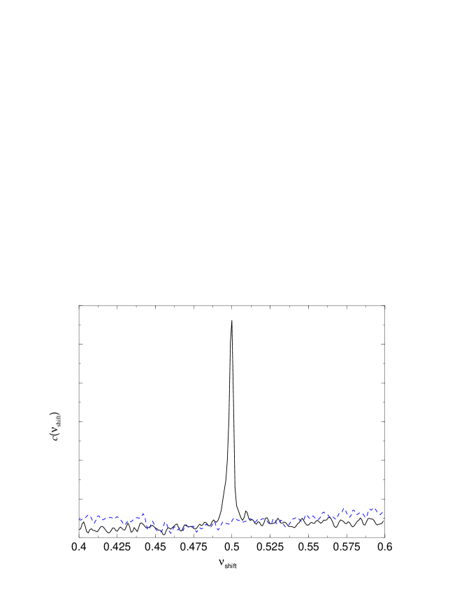
Figure 9.2: Cross-correlation function from Fig. 9.1 summed over integer shifts of the argument, $c(\nu_{\rm shift})=\sum_{n}C(n+\nu_{\rm shift})$, in order to focus on the positions of the peaks. In the double sum (9.4) the energies were taken within the same symmetry class (solid line) and between different symmetry classes (dotted line.)

In Figure 9.1 we show the cross-correlation function (9.4) for the ellipse billiard at magnetic length $b=0.1$. It was calculated from the edge spectra shown in Figures 7.3 and 7.6. The corresponding classical dynamics exhibits a strict one-to-one correspondence between the interior and the exterior classical dynamics up to $\nu=21.6$. Beyond this energy, when the cyclotron radius is greater than the minimum radius of curvature, the classical duality still holds in a substantial part of phase space. One observes that $C(\nu_{0})$ is strongly fluctuating and displays pronounced, equidistant peaks at energies $\nu_{0}=N+{\frac{1}{2}}$, as predicted by (9.14). In Figure 9.2 we focus on these dominant structures by plotting the cross-correlation function in terms of $\nu_{\rm shift}=\nu_{0}({\rm mod}\ 1)$ around one half. To check that the resulting correlation signal is not an artefact or due to the accumulation of bulk states we make use of the fact that the spectra of the ellipse decompose into two symmetry classes. As shown above (9.18) one expects $C(\nu_{0})$ to be structureless if one correlates edge spectra belonging to different symmetries. This is clearly supported by the numerical results shown as a dashed line in Figure 9.2.

\psfrag{t}{$t$}\psfrag{|D(t)|}{$|D(t)|$}\includegraphics[width=346.89731pt]{figs/D_s1_sum_h4g5e-4.eps}

Figure 9.3: Fourier transformation $D(t)$ (9.19) of the cross-correlation function $C(\nu_{0})$ given in Fig. 9.1 (absolute value). The peaks at integer $t$ correspond to the combined actions of dual periodic orbits ($\sigma_{g}=5\times~{}10^{-4}$, $\sigma_{h}=4$.)

The Fourier transform (9.19) of the cross-correlation function exposes the sums of actions of the contributing pairs of periodic orbits. The absolute value of $D(t)$, calculated for the same spectrum as Fig. 9.1, is shown in Figure 9.3. In this case, the periodic orbits of the de-symmetrized ellipse have at least $n_{\rm min}=4$ reflections. One observes that $|D(t)|$ displays distinct spikes at integer values. The real parts of the peaks have signs $(-)^{n}$, as expected from eq (9.16) (not shown). As predicted by the semiclassical theory the dominant peaks start at $n_{\rm min}=4$ which is a clear proof for the classical origin of the edge state correlations. The tiny peaks at $t=1,2,3$ vanish if one decreases the width of the window function $g$ (which in turn deteriorates the statistical significance of the result). They are due to the remnant contributions of the bulk states, and disappear if one removes the bulk states from the correlator sum by setting a threshold on the weights (not shown; the remaining peaks would not change by this procedure).

\psfrag{y}{$|D_{\rm mag}(t)|$}\psfrag{t}{$t$}\includegraphics[width=346.89731pt]{figs/mcorrellipseft.eps}

Figure 9.4: Fourier transform of the ellipse cross correlation function (9.1) for the ellipse defined in terms of the edge magnetization density. The graph should be compared to Fig. 9.3. ($\sigma_{g}=5\times 10^{-4}$, $\sigma_{h}=0.5$)

We repeated the calculation of the cross-correlation function of the ellipse spectrum now using $d_{\rm edge}^{\scriptscriptstyle(\mathcal{M})}(\nu)$ as the spectral measure. The resulting function exhibits peaks at the Landau energies similar to Fig. 9.1 (not shown). Its Fourier transform is given in Figure 9.4. Again, the peaks are located at integer values starting at $t=4$. This shows that the edge magnetization density $\widetilde{{\rm m}}_{\rm edge}$ succeeds to unravel the cross correlations similar to the edge density $d_{\rm edge}$ — a reassuring but not a surprising result.

\psfrag{x}{$\nu_{\rm shift}$}\psfrag{y}{$c(\nu_{\rm shift})$}\includegraphics[width=346.89731pt]{figs/mshift_stadium.eps}

Figure 9.5: Cross-correlation summed over integer shifts of the argument like in Fig. 9.2. The data belongs to the stadium billiard in Fig. 8.6 ($\nu=100-135$, $\sigma_{g}=5\times 10^{-4}$, $\sigma_{h}=0.2$, using the edge magnetization density (7.21).) A clear cross-correlation exists between energies of the same symmetry class (full line), while there is no signal if the energies are taken from different symmetry classes (dashed line.)

The ellipse spectrum considered so far exhibits generic, mixed chaotic dynamics with relatively large integrable parts in phase space. As the last point, we demonstrate that the correlations do exist also in a system which is completely chaotic. We choose the spectrum of the stadium billiard defined in Fig. 8.5 and use the edge magnetization to define the spectral density. As discussed in Chapter 8, the spectral interval shown in Fig. 8.6 corresponds to cyclotron radii large enough to ensure that the corresponding classical dynamics is essentially hyperbolic. Figure 9.5 gives the corresponding cross-correlation function. Like in Fig. 9.2 the variable is plotted modulo one in order to focus attention on the peaks. Again, we observe a clear cross-correlation signal for pairs within the same symmetry class (solid line) while the reference calculation from different symmetry classes shows no peak (dashed line).

9.3 The pair relation

Figure 9.6: For every correlated pair of interior and exterior edge energies, $\nu$ and $\nu^{\prime}$, there exists a Landau level $N+{\frac{1}{2}}$ such that the distances – scaled individually by the reciprocal quantum weights, $w$ and $w^{\prime}$ – coincide.

The peaks in $C(\nu_{0})$ were attributed to the complementarity of the actions of dual orbits. Quantum mechanically their occurrence implies that there exists a pairwise relation between individual interior and exterior edge states. This follows from the discussion of the quantum correlator (9.4) above. We have noted that pairs of edge energies contribute only if they have the same weighted distance to the reference energy from the left and right, respectively. Since the peaks appear at $\nu_{0}=N+\tfrac{1}{2}$ the interior energies $\nu_{i}$ and exterior energies $\nu_{j}^{\prime}$ must appear in pairs which satisfy

$$\frac{\nu_{i}-(N-\tfrac{1}{2})}{w_{i}}\cong\frac{(N-\tfrac{1}{2})-\nu_{j}^{\prime}}{w_{j}^{\prime}}$$ (9.22)

with integer $N$, see Fig. 9.6. Although this is not an exact relation, it will be the more precise the larger and the closer the two energies are, since the semiclassical approximation (7.2) and the linearization (9.1) then hold the better.

It is clear from (9.22) that the information provided by the ratio of the individual quantum weights plays a crucial role in unraveling this pair correlation. It explains why standard correlation functions, which involve unweighted densities, do not show any signal in general. Moreover, the fact that the quantum weights enter reciprocally in (9.22) explains how a pairwise relation between interior and exterior states can exist in spite of different local unweighted densities. It is consistent with the mean edge densities (7.4) being equal in the interior and exterior. Using the weights (7.23) which are based on the magnetization we obtain the same formula. It implies that for correlated pairs the individual ratios of the weights defined by (7.3) and by (7.23) are approximately equal. This is indeed observed numerically.

For a given interior edge state it is of course not known, a priori, which is the associated Landau level $N+{\frac{1}{2}}$ and the exterior weight. Therefore, even in an asymptotic sense it is not possible to infer an edge spectrum given the complementary one by just using the relation (9.22). However, having an interior and exterior edge spectrum available, one can decide whether they belong to the same billiard. In the spectra considered so far we could easily spot single pairs of edge states by just using the relation (9.22). Examples are given in Table 9.1.

Pair in Fig. 9.7 $\nu_{i}$ $w_{i}$ $\dfrac{\nu_{i}-\nu_{0}}{w_{i}}$ $\dfrac{\nu_{0}-\nu^{\prime}_{j}}{w^{\prime}_{j}}$ $w^{\prime}_{j}$ $\nu^{\prime}_{j}$ top $32.5367$ $0.826$ $0.0445$ $0.0444$ $0.506$ $32.4775$ middle $33.5248$ $0.489$ $0.0507$ $0.0501$ $0.533$ $33.4733$ bottom $32.5082$ $0.286$ $0.0288$ $0.0248$ $0.508$ $32.4874$

Table 9.1: Energies and weights of the correlated pairs in Fig. 9.7, with the primes indicating exterior states.

An alternative derivation of the pair relation

An independent semiclassical derivation of the pair relation (9.22) can be obtained without invoking periodic orbit theory by inspecting the semiclassical map operators $\mathsf{P}^{\rm int}$ and $\mathsf{P}^{\rm ext}$ of the interior and the exterior, see Sect. 6.2. We present here the derivation for the magnetization based weights (7.23), the calculation for the weights (7.3) is quite analogous. If follows from the discussion of (6.2) that the interior Dirichlet number counting function can be written in terms of the eigenphases $\theta_{\ell}(\nu;b^{2})$ of the unitary map operator $\mathsf{P}^{\rm int}$,

$${\rm N}_{\rm skip}^{\rm int}(\nu;b^{2})=\sum_{\ell}\Theta_{2\pi}\left(\theta_{\ell}(\nu;b^{2})+\pi\right)$$ (9.23)

where $\Theta_{2\pi}(\theta)$ is the unit staircase function at integer multiples of $2\pi$. The interior edge state density (7.22) is then given by

$$d_{\rm edge}^{{\scriptscriptstyle(\mathcal{M})}}(\nu;b^{2}) =-\frac{b^{2}}{\nu}\frac{\mathrm{d}}{\mathrm{d}b^{2}}{\rm N}_{\rm skip}^{\rm int}(\nu;b^{2})$$

$$=-\frac{b^{2}}{\nu}\sum_{\ell}\frac{\mathrm{d}\theta_{\ell}}{\mathrm{d}b^{2}}(\nu;b^{2})\,\delta_{2\pi}\left(\theta_{\ell}(\nu;b^{2})+\pi\right)\ ,$$ (9.24)

with $\delta_{2\pi}(\theta)=\frac{\mathrm{d}}{\mathrm{d}\theta}\Theta_{2\pi}(\theta)$ the $2\pi$-periodic $\delta$-function. The unweighted spectral density (3.9) is obtained in the same way by taking the derivative of (9.23) with respect to $\nu$. Comparing the two densities we conclude that the edge state weights are given by

$$w^{\rm{\scriptscriptstyle(\mathcal{M})}}=\left.-\frac{b^{2}}{\nu}\frac{\displaystyle\frac{\mathrm{d}\theta_{\ell}}{\mathrm{d}b^{2}}(\nu;b^{2})}{\displaystyle\frac{\mathrm{d}\theta_{\ell}}{\mathrm{d}\nu}(\nu;b^{2})}\right|_{\theta_{\ell}(\nu)=\pi\mod 2\pi}$$ (9.25)

The same equations hold for the exterior quantities (labeled by a prime) with a plus sign in (9.3) and (9.25). Now we make use of the duality relation (6.28) between the interior and the exterior map operators. It implies

$$\theta_{\ell}(\nu;b^{2})+\theta_{\ell}^{\prime}(\nu;b^{2})=2\pi\left(\nu-{\frac{1}{2}}\right)+2\pi\widetilde{M}\ .$$ (9.26)

with integer $\widetilde{M}$. Take a pair of interior and exterior energies $\nu$ and $\nu^{\prime}$ which are determined by the $\ell$th eigenphase, ie, $\theta_{\ell}(\nu)+\pi=2\pi M$ and $\theta^{\prime}_{\ell}(\nu^{\prime})+\pi=2\pi M^{\prime}$ with integer $M,M^{\prime}$. If we expand the eigenphases to first order around the Landau level $\nu+0=M+M^{\prime}-\widetilde{M}-{\frac{1}{2}}$ we obtain from (9.26)

$$\frac{\Delta\nu}{\Delta\nu^{\prime}}\cong-\frac{\tfrac{\mathrm{d}}{\mathrm{d}\nu}\theta^{\prime}_{\ell}(\nu_{0};b^{2})}{\tfrac{\mathrm{d}}{\mathrm{d}\nu}\theta_{\ell}(\nu_{0};b^{2})}=\frac{\tfrac{b^{2}}{\nu_{0}}\tfrac{\mathrm{d}}{\mathrm{d}b^{2}}\theta_{\ell}(\nu_{0};b^{2})/\tfrac{\mathrm{d}}{\mathrm{d}\nu}\theta_{\ell}(\nu_{0};b^{2})}{\tfrac{b^{2}}{\nu_{0}}\tfrac{\mathrm{d}}{\mathrm{d}b^{2}}\theta^{\prime}_{\ell}(\nu_{0};b^{2})/\tfrac{\mathrm{d}}{\mathrm{d}\nu}\theta^{\prime}_{\ell}(\nu_{0};b^{2})}\cong-\frac{w^{\scriptscriptstyle(\mathcal{M})}}{{w^{\scriptscriptstyle(\mathcal{M})}}^{\prime}}$$ (9.27)

with $\Delta\nu=\nu-\nu_{0}$ and $\Delta\nu^{\prime}=\nu^{\prime}-\nu_{0}$. The first equality holds if the distances to the Landau level $\Delta\nu$ and $\Delta\nu^{\prime}$ are sufficiently small. To the same degree of approximation we can replace the Landau energy $\nu_{0}$ by the eigenenergies $\nu$ and $\nu^{\prime}$ and using (9.25) we get the pair relation (9.22) in terms of the magnetic weights (last equality). The fact that it can be obtained without resorting to periodic orbit theory shows that the pairwise cross-correlation is a generic semiclassical feature of dual magnetic billiards and is not related to the type of the classical motion. We note that the duality relation (6.28) also implies that in the vicinity of a Landau level the operators $\mathsf{P}^{\rm int}$ and $\mathsf{P}^{\rm ext}$ are approximately inverse to each other. Hence, for correlated pairs of eigenstates the normal derivatives at the boundary are expected to be approximately equal (see the numerical test below).

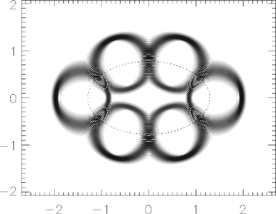
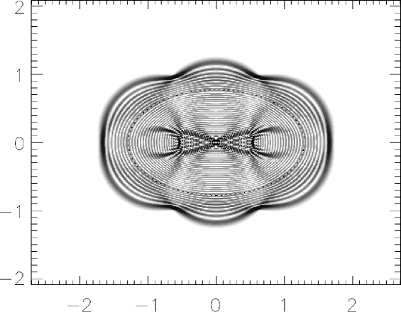
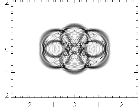
Figure 9.7: Pairs of correlated interior and exterior wave functions. The energies and weights are given Table 9.1. (Ellipse billiard at $b=0.1$; the shading is proportional to the modulus of the wave function, and the boundary is indicated by a dotted line.) [figure quality reduced]

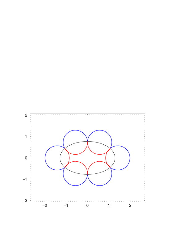
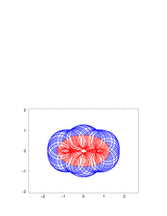
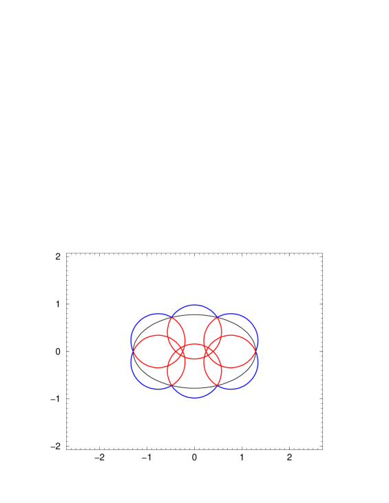
Figure 9.8: Dual pairs of classical periodic orbits in the ellipse billiard, at $\rho=0.57$. The top and bottom orbits are stable, while the middle one in unstable. Their classical weights (7.11) correspond to the quantum weights (7.3) of the states in Fig. 9.7.

Correlated wave functions

We proceed to present three pairs of correlated wave functions of the ellipse billiard. The interior states were chosen to have different locations in Figure 7.6 which displays the distribution of quantum weights on page 7.6 (top part). At energies corresponding to $\rho\approx 0.57$ we took states with weights lying in the top branch of the rightmost bifurcation structure, in the middle, and in the bottom branch, respectively. The respective correlated exterior states were identified using the pair relation (9.22). Table 9.1 lists the data for the three pairs.

Figure 9.7 displays superimpositions of the interior and the exterior wave functions. One clearly observes that the top and bottom wave functions are localized on dual periodic orbits. In agreement with this observation one finds that the structures of increased density of classical weights in Fig. 7.6 (page 7.6, bottom part) may be attributed to periodic orbits which bifurcate as the cyclotron radius $\rho$ is increased. The top and bottom wave functions were taken from a fork which belongs to orbits with period 6. Two of these orbits are shown in Fig. 9.8 along with their dual partners.

The middle wave functions in Figure 9.7, in contrast, are localized on a chaotic region in phase space confined by un-destroyed invariant tori. For comparison, an unstable pair of dual classical orbits from this region is given in the middle part of Fig. 9.8. Note that it exhibits the same spatial extension as the wave functions. Here, the correlation of interior and exterior wave functions is not evident from the visual inspection.

\psfrag{y}{$|\partial_{n/b}\psi-\mathrm{i}\tilde{A}_{n}\psi|$}\psfrag{s}{$s$}\includegraphics[width=433.62pt]{figs/on_boundary_mpair1.eps}

Figure 9.9: Boundary functions $|u|=|\partial_{n/b}\psi-\mathrm{i}\tilde{A}_{n}\psi|$ of the correlated wave functions depicted in Fig. 9.10 (along one half of the boundary). Solid line: interior ($\nu=110.6567$), dotted line: exterior ($\nu^{\prime}=110.4841$). The difference is given as a dashed line.

\psfrag{-4}{$-4$}\psfrag{-2}{$-2$}\psfrag{0}{$0$}\psfrag{2}{$2$}\psfrag{4}{$4$}\includegraphics[width=433.62pt]{figs/s14_mpair1_auschnitt_66dpi.eps}

Figure 9.10: A typical pair of correlated wave functions taken from the spectrum displayed in Fig. 8.6 (superimposed; $\nu=110.6567$, $\nu^{\prime}=110.4841$, $b=0.2$). The stadium-shaped boundary is not drawn but visible as a regular nodal line. Figure 9.11 shows the pair on a larger scale. [figure quality reduced]

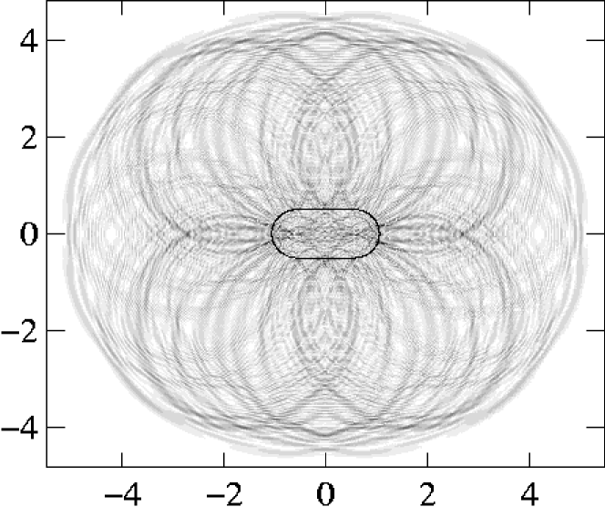
Figure 9.11: The pair of correlated interior and exterior wave functions from Fig. 9.10 on a larger scale. The black line indicates the stadium-shaped boundary. The circular scars in the exterior wave function match the classical cyclotron radius $\rho\simeq 2.10\,$. [figure quality reduced]

The most convincing evidence for the correlation between interior and exterior eigenfunctions comes from a striking similarity of their respective normal derivatives at the boundary. This is a feature shared by all pairs of correlated wave functions, including those which are based on a chaotic part of the phase space. To show this clearly we compare in Fig. 9.9 the normal derivatives of a typical pair of correlated states taken from the stadium billiard. One observes that the moduli resemble each other, even though they are rather irregular. The difference of the interior and the exterior values is indicated by the dashed line. As a consequence of (9.22) one expects in general that the difference is the smaller the closer two edge states are in energy. If the edge energies happened to coincide this would have to take place on a Landau level according to (9.22) and the continuation of one wave function would simply yield the other, ie the normal derivatives would coincide.

In Figure 9.10 we show the wave functions of the pair from the stadium billiard for which the boundary functions are shown in Fig. 9.9. Although they exhibit the typical irregular pattern of wave function based on a chaotic part of phase space, one can notice that the interior and exterior structures match. In the exterior wave function scars of periodic orbits may be discerned if viewed with some measure of imagination, see Fig. 9.11. Here, the circular structures match the classical cyclotron radius $\rho\cong 2.10$.

10 Conclusions

The main goal of this review was to present a practical and coherent theoretical framework for the study of magnetic edge states allowing in particular the investigation of their semiclassical properties. An important step was to set up a quantitative and physically meaningful definition for the notion of edge states. It became the crucial ingredient for identifying the quantum analogue of the classical interior-exterior duality. In the remainder we discuss a few of the unsettled problems and comment on possible new directions of research motivated by the progress made so far.

The boundary integral method presented in Chapter 4 was formulated only for smooth boundaries. This restriction was crucial for the regularization of the hypersingular integral operators, which is necessary at non-Dirichlet boundary conditions, and a general treatment of corners or cusps is still missing. Also the effect of the general boundary conditions on the smooth number counting function was computed indirectly only. Balian and Bloch and others developed a systematic method for the computation of these quantities [75, 76] which should be extended to the magnetic case. The implementation of this program is technically far from being simple and awaits a proper treatment.

As a natural direction of further research one should ask whether the proposed spectral measure is applicable and useful in other areas, specifically for the physics of the (fractional) Quantum Hall effect, where the concept of edge states is frequently employed without a clear definition. The introduction of confining walls which extend to infinity adds an essentially new dimension to the study of edge states. It requires a scattering theory appropriate to the continuous spectrum encountered in such systems. The models investigated so far dealt with the simplest geometries[131, 132]. Once an obstacle (ie, a billiard) is placed near a wall or between parallel walls, scattering resonances will appear. Their analysis is important from an experimental point of view and theoretically challenging since they introduce resonant transitions between counter-propagating modes along adjacent leads. In the field-free case the scattering matrix is often discussed in terms of boundary integrals, and we expect that the techniques developed in Chapter 4 may provide convenient tools for the corresponding magnetic scattering theory — the same holds for the development a semiclassical scattering theory. These problems are bound to find applications for magneto-transport experiments involving ballistic mesoscopic devices.

The quantum interior-exterior duality belongs to a more general class of problems emerging in the field of quantum chaos. Here, one considers systems whose classical dynamics are related in some way and asks for the quantum correlations implied by the classical correlations and how they emerge in the semiclassical limit. Recently B. Gutkin analyzed the boundary operators for a line partitioning the $2d$-sphere [133] and found that the corresponding semiclassical map operators are related by an analogue of Equation (6.28). More complicated surfaces or the consequences of other classical relations were not yet analyzed but are a natural direction of further research.

Appendix A Appendices

A.1 Green function in angular momentum representation

In Section 2.5 the magnetic Green function was obtained by a direct evaluation of the Fourier integral. In the present appendix we derive its angular momentum decomposition. This lets us correct some erroneous results in the literature and discuss the irregular Green function. Moreover, the solutions of the radial Schrödinger equation will be needed below, in App. A.3.

The symmetric gauge must be employed since only this choice renders the angular momentum a constant of the motion. In polar coordinates the inhomogeneous Schrödinger equation (2.50) then assumes the form

$$\Big{[}-\frac{1}{4}(\partial^{2}_{{\tilde{r}}}+\frac{1}{{\tilde{r}}}\partial_{{\tilde{r}}})+\frac{1}{4}({\tilde{r}}+\mathrm{i}\frac{\partial_{\vartheta}}{{\tilde{r}}})^{2}-\nu\Big{]}{\rm G}_{\nu}=-\frac{1}{4}\,\delta(\tilde{\mathbf{r}}-\tilde{\mathbf{r}}_{0})\ .$$ (A.1)

An ansatz in terms of the difference of polar angles,

$${\rm G}_{\nu}(\mathbf{r},\mathbf{r}_{0})=\frac{1}{2\pi}\sum_{m=-\infty}^{\infty}\mathrm{e}^{\mathrm{i}m(\vartheta-\vartheta_{0})}G_{m}({\tilde{r}},{\tilde{r}}_{0})\ ,$$ (A.2)

which cannot be justified a priori, separates the radial and the angular coordinates. For ${\tilde{r}}\neq{\tilde{r}}_{0}$ the functions $G_{m}$ solve the radial Schrödinger equation in the plane

$$\Big{[}\partial^{2}_{{\tilde{r}}}+\frac{1}{{\tilde{r}}}\partial_{{\tilde{r}}}-\frac{({\tilde{r}}^{2}-m)^{2}}{{\tilde{r}}^{2}}+4\nu\Big{]}G_{m}({\tilde{r}},{\tilde{r}}_{0})=0\ .$$ (A.3)

The definition

$$G_{m}({\tilde{r}},{\tilde{r}}_{0})={\tilde{r}}^{|m|}\,\mathrm{e}^{-{\tilde{r}}^{2}/2}\,g_{m}({\tilde{r}}^{2})$$ (A.4)

leads to an equation for $g_{m}$,

$$zg_{m}^{\prime\prime}(z)+(1+|m|-z)g_{m}^{\prime}(z)-\Big{(}{\frac{1}{2}}-\nu+\frac{|m|-m}{2}\Big{)}g_{m}(z)=0\ ,$$ (A.5)

which is known as Kummer’s differential equation and is solved by the regular and irregular hypergeometric function, $\mathop{{{}_{1\,}{\!\rm F}_{\!1}}}\nolimits$ and ${\rm U}$, respectively [36]. For energies different from the Landau levels it follows that a pair of independent solutions $u_{1},u_{2}$ of the radial Schrödinger equation (A.3) is given by

$$u_{1}({\tilde{r}}) ={\tilde{r}}^{|m|}\,\mathrm{e}^{-{\tilde{r}}^{2}/2}\,\mathop{{{}_{1\,}{\!\rm F}_{\!1}}}\nolimits\Big{(}{\frac{1}{2}}-\nu+\frac{|m|-m}{2},1+|m|,{\tilde{r}}^{2}\Big{)}$$ (A.6)

and

$$u_{2}({\tilde{r}}) ={\tilde{r}}^{|m|}\,\mathrm{e}^{-{\tilde{r}}^{2}/2}\,{\rm U}\Big{(}{\frac{1}{2}}-\nu+\frac{|m|-m}{2},1+|m|,{\tilde{r}}^{2}\Big{)}\ .$$ (A.7)

Both are real valued solutions. $u_{1}$ is bounded at ${\tilde{r}}=0$ and diverges as ${\tilde{r}}\to\infty$. The function $u_{2}$, on the other hand, decays like a Gaussian in this limit but displays a (logarithmic) singularity as ${\tilde{r}}\to 0$.

Another fundamental system of equation (A.3) is obtained if one replaces $u_{2}$ by

$$u^{\rm irr}_{2}({\tilde{r}}) ={\tilde{r}}^{|m|}\,\mathrm{e}^{+{\tilde{r}}^{2}/2}\,{\rm U}\Big{(}{\frac{1}{2}}+\nu+\frac{|m|+m}{2},1+|m|,-{\tilde{r}}^{2}\Big{)}\ .$$ (A.8)

This is a complex valued solution [134] which we call “irregular”. Apart from its logarithmic singularity at ${\tilde{r}}\to 0$, it diverges exponentially as ${\tilde{r}}\to\infty$.

Both $u_{1}$ and $u_{2}$ are needed to form a solution $G_{m}$ of the inhomogeneous equation (A.1) since the $\delta$-function implies a discontinuity of the derivative,

$$\partial_{1}G_{m}({\tilde{r}}_{0}+0,{\tilde{r}}_{0})-\partial_{1}G_{m}({\tilde{r}}_{0}-0,{\tilde{r}}_{0})=\frac{1}{{\tilde{r}}_{0}}\ .$$ (A.9)

The requirement that the Green function must vanish as ${\tilde{r}}\to\infty$, together with its continuity at ${\tilde{r}}={\tilde{r}}_{0}$, leads necessarily to the form

$$G_{m}({\tilde{r}},{\tilde{r}}_{0})=\frac{1}{{\tilde{r}}_{0}W({\tilde{r}}_{0})}\begin{cases}u_{1}({\tilde{r}})u_{2}({\tilde{r}}_{0})&\text{if $r<r_{0}$}\\ u_{2}({\tilde{r}})u_{1}({\tilde{r}}_{0})&\text{if $r>r_{0}$\ ,}\end{cases}$$ (A.10)

with Wronskian $W=u_{1}u_{2}^{\prime}-u_{1}^{\prime}u_{2}$. In total, the Green function in angular momentum decomposition and symmetric gauge is given by

$${\rm G}_{\nu}(\mathbf{r};\mathbf{r}_{0}) =\frac{-1}{4\pi}\sum_{m=-\infty}^{\infty}\!\!\mathrm{e}^{\mathrm{i}m(\vartheta-\vartheta_{0})}\,\frac{\Gamma\Big{(}{\frac{1}{2}}-\nu+\frac{|m|-m}{2}\Big{)}}{|m|!}\,\Big{(}\frac{rr_{0}}{b^{2}}\Big{)}^{|m|}\exp\Big{(}-\frac{r^{2}+r_{0}^{2}}{2b^{2}}\Big{)}$$

$$\phantom{\frac{-1}{4\pi}\sum_{m=-\infty}^{\infty}}\times\mathop{{{}_{1\,}{\!\rm F}_{\!1}}}\nolimits\Big{(}{\frac{1}{2}}-\nu+\frac{|m|-m}{2},1+|m|,z_{<}\Big{)}$$

$$\phantom{\frac{-1}{4\pi}\sum_{m=-\infty}^{\infty}}\times{\rm U}\Big{(}{\frac{1}{2}}-\nu+\frac{|m|-m}{2},1+|m|,z_{>}\Big{)}$$ (A.11)

$$=\frac{-1}{4\pi}\sum_{m=-\infty}^{\infty}\!\!\mathrm{e}^{\mathrm{i}m(\vartheta-\vartheta_{0})}\,\frac{\Gamma\Big{(}{\frac{1}{2}}-\nu+\frac{|m|-m}{2}\Big{)}}{|m|!}\,\Big{(}\frac{rr_{0}}{b^{2}}\Big{)}^{-1}\,M_{\nu+\frac{m}{2},\frac{|m|}{2}}(z_{<})\;$$

$$\phantom{\frac{-1}{4\pi}\sum_{m=-\infty}^{\infty}}\times W_{\nu+\frac{m}{2},\frac{|m|}{2}}(z_{>})$$ (A.12)

with $M_{k,\mu}(z)$ and $W_{k,\mu}(z)$ the regular and irregular Whittaker functions [36], and

$$z_{<} :=\min\left(\frac{\mathbf{r}^{2}}{b^{2}},\frac{\mathbf{r}_{0}^{2}}{b^{2}}\right)\quad\text{and}\quad z_{>}:=\max\left(\frac{\mathbf{r}^{2}}{b^{2}},\frac{\mathbf{r}_{0}^{2}}{b^{2}}\right)\ .$$ (A.13)

Note that this expression differs slightly from the (incorrect) expressions in [32] and [26, eq (6.2.26)].

An independent solution to the inhomogeneous problem (A.1) may obtained if one drops the requirement that the Green function should vanish as ${\tilde{r}}\to\infty$. It involves the irregular solution (A.8) and leads to the Green function

$${\rm G}^{\rm(irr)}_{\nu}(\mathbf{r};\mathbf{r}_{0}) =\frac{-1}{4\pi}\sum_{m=-\infty}^{\infty}\!\!\mathrm{e}^{\mathrm{i}(\vartheta-\vartheta_{0}+\pi)m}\,\frac{\Gamma\Big{(}{\frac{1}{2}}+\nu+\frac{|m|+m}{2}\Big{)}}{|m|!}\,\Big{(}\frac{rr_{0}}{b^{2}}\Big{)}^{|m|}\exp\Big{(}\frac{r^{2}+r_{0}^{2}}{2b^{2}}\Big{)}$$

$$\phantom{\frac{-1}{4\pi}\sum_{m=-\infty}^{\infty}}\times\mathop{{{}_{1\,}{\!\rm F}_{\!1}}}\nolimits\Big{(}{\frac{1}{2}}+\nu+\frac{|m|+m}{2},1+|m|,-z_{<}\Big{)}$$

$$\phantom{\frac{-1}{4\pi}\sum_{m=-\infty}^{\infty}}\times{\rm U}\Big{(}{\frac{1}{2}}+\nu+\frac{|m|+m}{2},1+|m|,-z_{>}\Big{)}$$ (A.14)

which we call “irregular”. This expression was derived by Tiago et al.[33]. Unlike the regular Green function (A.1), this one diverges exponentially once the distance between initial and final point exceeds one cyclotron diameter. This property renders the irregular Green function impractical for most purposes.

A.2 The null field method

The null field method is an alternative scheme to quantize magnetic billiards in the interior [33]. We include it for completeness although its practical use is limited.

Let us start with equation (4.4). In terms of the irregular Green function it reads

$$\int_{\Gamma}{\rm G}^{\rm(irr)}_{\nu}(\mathbf{r};\mathbf{r}_{0})\partial_{n/b}\psi^{*}\frac{\mathrm{d}\Gamma}{b}=0\ ,$$ (A.15)

where we chose $\mathbf{r}_{0}\in{{{\mathbb{R}}}^{2}}\setminus\mathcal{D}$, Dirichlet boundary conditions, and the symmetric gauge. Rather than transforming this into an integral equation we place $\mathbf{r}_{0}$ on a (large) circle with radius $R_{p}$ which is centered at the origin and surrounds the billiard domain.

Now assume that the billiard boundary is given as a function $r(\theta)$ of the polar angle and expand the unknown boundary function in a Fourier series,

$$\partial_{n/b}\psi^{*}\big{(}r(\theta)\big{)}=\sum_{\ell}\mathrm{e}^{\mathrm{i}\theta\ell}c_{\ell}\ .$$ (A.16)

Using the angular momentum decomposition (A.1) of the irregular Green function equation (A.15) assumes the form

$$\sum_{\ell,m=-\infty}^{\infty}\mathrm{e}^{-\mathrm{i}\theta_{0}m}a_{m}B_{m\ell}c_{\ell}=0\ ,$$ (A.17)

with

$$a_{m}= \,(-)^{m}\frac{\Gamma\Big{(}{\frac{1}{2}}+\nu+\frac{|m|+m}{2}\Big{)}}{|m|!}\,\Big{(}\frac{R_{p}}{b^{2}}\Big{)}^{|m|}\exp\Big{(}\frac{R_{p}^{2}}{2b^{2}}\Big{)}$$

$$\,\times{\rm U}\Big{(}{\frac{1}{2}}+\nu+\frac{|m|+m}{2},1+|m|,-\frac{R_{p}^{2}}{b^{2}}\Big{)}$$ (A.18)

and

$$B_{m\ell}= \,\int_{0}^{2\pi}\!\!\mathrm{e}^{\mathrm{i}(m+\ell)\theta}\,\Big{(}\frac{r(\theta)}{b^{2}}\Big{)}^{|m|}\exp\Big{(}\frac{r^{2}(\theta)}{2b^{2}}\Big{)}$$

$$\,\times\mathop{{{}_{1\,}{\!\rm F}_{\!1}}}\nolimits\Big{(}{\frac{1}{2}}+\nu+\frac{|m|+m}{2},1+|m|,-\frac{r^{2}(\theta)}{b^{2}}\Big{)}\,\mathrm{d}\theta$$ (A.19)

$$= \,\int_{0}^{2\pi}\!\!\mathrm{e}^{\mathrm{i}(m+\ell)\theta}\,\Big{(}\frac{r(\theta)}{b^{2}}\Big{)}^{|m|}\exp\Big{(}-\frac{r^{2}(\theta)}{2b^{2}}\Big{)}$$

$$\,\times\mathop{{{}_{1\,}{\!\rm F}_{\!1}}}\nolimits\Big{(}{\frac{1}{2}}-\nu+\frac{|m|-m}{2},1+|m|,\frac{r^{2}(\theta)}{b^{2}}\Big{)}\,\mathrm{d}\theta\ .$$ (A.2a)

Equation (A.17) holds for all polar angles $\theta_{0}$. For negative arguments the function ${\rm U}$ is known to be complex and non-zero [134]. Therefore we can divide by $a_{m}$ for all $R_{p}$ which leaves the condition for the existence of a nontrivial solution $c_{\ell}$ to

$$\det(B_{m\ell})=0\ .$$ (A.20)

This is a spectral equation which was derived by Tiago et al. [33] (except for a misprint in their paper).

A.3 Exact quantization of the magnetic disk

We briefly describe how to quantize the interior and the exterior of the magnetic disk. As discussed in Sect. 6.5, the problem is separable in the symmetric gauge. For this choice the exact solutions of the free Schrödinger equation are given above, see (A.6) and (A.7). It follows that the interior and the exterior eigenfunctions of the disk are specified uniquely by their behavior at the origin and at infinity, respectively, and by the angular momentum quantum number $m$. Since the interior wave function (at energy $\nu$) must be regular at the origin it has the form

$$\psi_{m}(r,\vartheta)=\mathcal{N}_{\rm int}\,\mathrm{e}^{\mathrm{i}m\vartheta}\,\Big{(}\frac{r}{b}\Big{)}^{|m|}\,\mathrm{e}^{-\tfrac{r^{2}}{2b^{2}}}\,\mathop{{{}_{1\,}{\!\rm F}_{\!1}}}\nolimits\!\Big{(}{\frac{1}{2}}-\nu+\frac{|m|-m}{2},1+|m|;\frac{r^{2}}{b^{2}}\Big{)}\ .$$ (A.21)

For the exterior wave function, which must vanish at infinity, we have

$$\psi_{m}(r,\vartheta)=\mathcal{N}_{\rm ext}\,\mathrm{e}^{\mathrm{i}m\vartheta}\,\Big{(}\frac{r}{b}\Big{)}^{|m|}\,\mathrm{e}^{-\tfrac{r^{2}}{2b^{2}}}\,{\rm U}\Big{(}{\frac{1}{2}}-\nu+\frac{|m|-m}{2},1+|m|;\frac{r^{2}}{b^{2}}\Big{)}\ .$$ (A.22)

Upon applying the general boundary conditions (3.6) at the disk radius $r=R$ one obtains the spectral functions

$$\xi_{\rm disk}\Big{(}\nu;m,\Lambda,\frac{R}{b}\Big{)} =\Big{[}\sqrt{\nu}+(\pm\Lambda)\Big{(}\frac{R}{2b}-\frac{|m|b}{2R}\Big{)}\Big{]}K\Big{(}{\frac{1}{2}}-\nu+\frac{|m|-m}{2},1+|m|;\frac{R^{2}}{b^{2}}\Big{)}$$

$$-(\pm\Lambda)\frac{R}{b}\,\partial_{3}K\Big{(}{\frac{1}{2}}-\nu+\frac{|m|-m}{2},1+|m|;\frac{R^{2}}{b^{2}}\Big{)}$$ (A.23)

with

$$K(a,b;z) =\begin{cases}\mathop{{{}_{1\,}{\!\rm F}_{\!1}}}\nolimits(a,b;z)&\text{for the interior problem}\\ {\rm U}(a,b;z)&\text{for the exterior problem.}\end{cases}$$ (A.24)

($\partial_{j}K$ indicates partial derivation with respect to the $j$th argument.) Unlike the semiclassical case (6.98), one cannot predetermine the radial quantum number here but has to search for all zeros at given angular quantum number $m$. The derivatives of the energies with respect to external parameters are given explicitely by derivatives of the spectral function like in the semiclassical case. For variations in the boundary condition we find

$$\left.\frac{\mathrm{d}\nu}{\mathrm{d}\Lambda}\right|_{\Lambda=0}=\mp\frac{R}{\sqrt{\nu}b}\,\frac{\partial_{3}K}{\partial_{1}K}$$ (A.25)

with the arguments of $K$ like above. Similarly, the derivatives with respect to the magnetic length are given by the quotient

$$b^{2}\frac{\mathrm{d}\nu}{\mathrm{d}b^{2}}=-\frac{R^{2}}{b^{2}}\,\frac{\partial_{3}K}{\partial_{1}K}\ .$$ (A.26)

We note the relation

$$b^{2}\frac{\mathrm{d}\nu}{\mathrm{d}b^{2}}=\pm\sqrt{\nu}\,\frac{R}{b}\left.\frac{\mathrm{d}\nu}{\mathrm{d}\Lambda}\right|_{\Lambda=0}$$ (A.27)

which holds in the semiclassical case as well.

A.4 The stationary phase approximation

The method of the stationary phase yields asymptotic expansions of integrals with rapidly oscillating integrands like $\int\!g({x})\mathrm{e}^{2\pi\mathrm{i}\nu f({x})}\mathrm{d}{x}$. One can show that for large $\nu$ the leading order contribution stems from the stationary points of the phase $f$. After an expansion of the phase to second order around these points and the use of the Gaussian integral

$$\int_{-\infty}^{\infty}\mathrm{e}^{\textstyle\mathrm{i}ax^{2}}\mathrm{d}x=\left(\frac{\pi}{|a|}\right)^{\frac{1}{2}}\mathrm{e}^{\textstyle\mathrm{i}\mathop{\mathrm{sgn}}\nolimits(a)\frac{\pi}{4}}$$ (A.28)

one finds that for functions $f,g\in C^{\infty}(\mathbb{R})$ where $f$ has a finite number of non-degenerate stationary points ${x}_{j}$, ie, $f^{\prime}({x}_{j})=0$, the asymptotic expansion reads [135]

$$\int\!\!g({x})\mathrm{e}^{2\pi\mathrm{i}\nu f({x})}\mathrm{d}{x}=\frac{1}{\sqrt{\nu}}\sum_{{x}_{j}}\frac{g({x}_{j})}{|f^{\prime\prime}({x}_{j})|^{\frac{1}{2}}}\mathrm{e}^{2\pi\mathrm{i}\nu f({x}_{j})+\mathrm{i}\frac{\pi}{4}\mathop{\mathrm{sgn}}\nolimits(f^{\prime\prime}({x}_{j}))}\,\big{(}1+\mathord{\mathrm{O}}({\nu}^{-1})\big{)}\ ,$$ (A.29)

as $\nu\to\infty$. For functions of an $N$-dimensional argument, $f,g\in C^{\infty}(\mathbb{R}^{N})$, an analogous form can be found [136]:

$$\int\!\!g(\mathbf{x})\mathrm{e}^{2\pi\mathrm{i}\nu f(\mathbf{x})}\mathrm{d}^{N}\mathbf{x}\sim\left(\frac{\mathrm{i}}{\nu}\right)^{\frac{N}{2}}\sum_{\mathbf{x}_{j}}\frac{g(\mathbf{x}_{j})}{|\det f^{\prime\prime}(\mathbf{x}_{j})|^{\frac{1}{2}}}\mathrm{e}^{2\pi\mathrm{i}\nu f(\mathbf{x}_{j})-\mathrm{i}\nu_{j}\frac{\pi}{2}}\ .$$ (A.30)

Here, $\nu_{j}$ gives the number of negative eigenvalues of the matrix $f^{\prime\prime}(\mathbf{x}_{j})$.

A peculiar $\boldsymbol{\delta}$-function

As an immediate application the stationary phase approximation allows to show that the complex function

$$\delta_{\varepsilon}(\xi):=\frac{1}{(2\pi\mathrm{i})^{\frac{1}{2}}}\frac{\exp\left({\mathrm{i}\,\frac{\xi^{2}}{2\varepsilon}}\right)}{\sqrt{\varepsilon}}$$ (A.31)

has the property of a one-dimensional Dirac $$\delta$$-function,

$$\int\delta_{\varepsilon}(\xi)\,\mathrm{d}\xi=1$$ (A.32)

$$\int g(\xi)\,\delta_{\varepsilon}(\xi)\,\mathrm{d}\xi=g(0)\,(1+\mathord{\mathrm{O}}(\varepsilon))\qquad\text{as $\varepsilon\to 0$.}$$ (A.32a)

This follows from (A.28) and (A.29), with $\nu=1/\varepsilon$ and $f=x^{2}/2$, and is not easily proven otherwise. The product of (A.31) for the two Cartesian components of the vector $\mathbf{r}$ yields the two dimensional $\delta$-function

$$\lim_{\varepsilon\to 0}\frac{1}{2\pi\mathrm{i}b^{2}}\,\frac{1}{\varepsilon}\exp\left[\mathrm{i}\frac{(\mathbf{r}-\mathbf{r}_{0})^{2}}{2\varepsilon b^{2}}\right]=\delta(\mathbf{r}-\mathbf{r}_{0})\ ,$$ (A.33)

which shows up in (2.4).

A.5 The product relation of the map operators

We show that the relations (6.25) for the products of the interior and exterior map operators (6.2) hold semiclassically. They were needed to prove the factorization of the spectral function. Since possible saddle point contributions are excluded by the vanishing prefactors and the duality condition the only relevant contribution to the product stems from regions where the initial and the final point are close. Hence, we are allowed to replace the boundary locally by a circular arc. It follows that the expressions (6.72) – (6.75) derived for the disk billiards may be employed to show that the kernel of the product (6.25) acts like a $\delta$-function. Assuming the angle between the initial and the final point $\delta\varphi=(s-s_{0})/R$ to be small we find

$$\left({\rm p}_{\rm S}^{\rm int}{\rm p}_{\rm L}^{\rm ext}\right)(s,s_{0})=$$

$$= \frac{1}{2\pi\mathrm{i}}\,\frac{b}{R}\int\mathrm{d}\varphi^{\prime}\left(\frac{\mathrm{d}^{2}(2\pi\nu{\rm a}_{\rm S})}{\mathrm{d}\varphi\,\mathrm{d}\varphi_{0}}(\varphi^{\prime}-\varphi_{0})\,\frac{\mathrm{d}^{2}(2\pi\nu{\rm a}_{\rm L})}{\mathrm{d}\varphi_{0}\,\mathrm{d}\varphi^{\prime}}(\varphi_{0}+\delta\varphi-\varphi^{\prime})\right)^{\frac{1}{2}}$$

$$\times\mathrm{e}^{2\pi\mathrm{i}\nu({\rm a}_{\rm S}(\varphi^{\prime}-\varphi_{0})+{\rm a}_{\rm L}(\varphi_{0}+\delta\varphi-\varphi^{\prime}))}\begin{cases}-\Theta(\varphi^{\prime}-\varphi_{0})\Theta(\varphi^{\prime}-\varphi_{0}+\delta)&\text{if $\Gamma_{\!\rm d}>1$}\\ -1&\text{if $\Gamma_{\!\rm d}<1$}\end{cases}$$

$$\simeq \frac{1}{\pi}\,\frac{b\nu}{R}\int\mathrm{d}\varphi^{\prime}\left|\frac{\mathrm{d}^{2}(\pi{\rm a}_{\rm L})}{\mathrm{d}\varphi^{\prime}\,\mathrm{d}\varphi_{0}}(\varphi_{0}-\varphi^{\prime})\right|\mathrm{e}^{2\pi\mathrm{i}\nu+2\pi\mathrm{i}\nu\partial_{\varphi_{0}}{\rm a}_{\rm L}(\varphi_{0}-\varphi^{\prime})\,\delta\varphi}\begin{cases}-\Theta(\varphi^{\prime}-\varphi_{0})\\ -1\end{cases}$$

$$= \frac{1}{\pi}\,\frac{b\nu}{R}\,\mathrm{e}^{2\pi\mathrm{i}\nu}\int\mathrm{d}\varphi^{\prime}\,\frac{\mathrm{d}u_{\rm L}}{\mathrm{d}\varphi^{\prime}}\,\mathrm{e}^{2\mathrm{i}\nu u_{\rm L}\,\delta\varphi}\begin{cases}\Theta(\varphi^{\prime}-\varphi_{0})&\text{if $\Gamma_{\!\rm d}>1$}\\ 1&\text{if $\Gamma_{\!\rm d}<1$\ .}\end{cases}$$ (A.34)

with $\Gamma_{\!\rm d}=R/(b\nu^{\frac{1}{2}})$, see (6.64). The dependence on $\delta\varphi$ was expanded linearly in the phase and neglected in the prefactor. The latter is cancelled by the change of the integration variable to $u_{\rm L}:=\pi\partial_{\varphi_{0}}{\rm a}_{\rm L}(\varphi_{0}-\varphi^{\prime})$. Likewise, one finds for the second combination of interior and exterior operators:

$$\left({\rm p}_{\rm L}^{\rm int}{\rm p}_{\rm S}^{\rm ext}\right)(s,s_{0})=\frac{1}{\pi}\,\frac{b\nu}{R}\,\mathrm{e}^{2\pi\mathrm{i}\nu}\int\mathrm{d}\varphi^{\prime}\,\frac{\mathrm{d}u_{\rm S}}{\mathrm{d}\varphi^{\prime}}\,\mathrm{e}^{2\mathrm{i}\nu u_{\rm S}\,\delta\varphi}\begin{cases}-\Theta(\varphi^{\prime}-\varphi_{0})&\text{if $\Gamma_{\!\rm d}>1$}\\ 0&\text{if $\Gamma_{\!\rm d}<1$\ ,}\end{cases}$$

with $u_{\rm S}:=\pi\partial_{\varphi_{0}}{\rm a}_{\rm S}(\varphi_{0}-\varphi^{\prime})$. The sum of the kernels assumes the form of a semiclassical $\delta$-function once the integration is carried out. The ranges of integration differ for weak and strong fields. They can be found in Table A.1. Setting ${\overline{\varphi}}\equiv 2\arcsin(1/\Gamma_{\!\rm d})$ one gets

$$\big{(}{\rm p}_{\rm S}^{\rm int} {\rm p}_{\rm L}^{\rm ext}+{\rm p}_{\rm L}^{\rm int}{\rm p}_{\rm S}^{\rm ext}\big{)}(s,s_{0})=$$

$$=\frac{1}{\pi}\,\frac{b\nu}{R}\,\mathrm{e}^{2\pi\mathrm{i}\nu}\begin{cases}\displaystyle\int_{\Gamma_{\!\rm d}+{\frac{1}{2}}\Gamma_{\!\rm d}^{2}}^{{\frac{1}{2}}\Gamma_{\!\rm d}^{2}\cos({\overline{\varphi}})}\mathrm{d}u_{\rm L}\,\mathrm{e}^{2\mathrm{i}\nu u_{\rm L}\delta\varphi}-\int_{-\Gamma_{\!\rm d}+{\frac{1}{2}}\Gamma_{\!\rm d}^{2}}^{{\frac{1}{2}}\Gamma_{\!\rm d}^{2}\cos({\overline{\varphi}})}\mathrm{d}u_{\rm S}\,\mathrm{e}^{2\mathrm{i}\nu u_{\rm S}\delta\varphi}&\text{if $\Gamma_{\!\rm d}>1$}\\[10.76385pt] \displaystyle\int_{\Gamma_{\!\rm d}+{\frac{1}{2}}\Gamma_{\!\rm d}^{2}}^{-\Gamma_{\!\rm d}+{\frac{1}{2}}\Gamma_{\!\rm d}^{2}}\mathrm{d}u_{\rm L}\,\mathrm{e}^{2\mathrm{i}\nu u_{\rm L}\delta\varphi}&\text{if $\Gamma_{\!\rm d}<1$}\end{cases}$$

$$=-\,\mathrm{e}^{2\pi\mathrm{i}\nu}\,\frac{1}{\pi}\,\frac{\sin\left(2\sqrt{\nu}\,\frac{s-s_{0}}{b}\right)}{\frac{s-s_{0}}{b}}\,\mathrm{e}^{\mathrm{i}\pi\sqrt{\nu}\Gamma_{\!\rm d}(s-s_{0})/b}\begin{CD}@>{2\sqrt{\nu}\to\infty}>{}>\end{CD}-\,\mathrm{e}^{2\pi\mathrm{i}\nu}\,{\delta}\!\left(\frac{s-s_{0}}{b}\right)\ .$$ (A.36)

This proves the identity (6.25). In a similar fashion one finds that the product (6.26) does not contribute semiclassically.

If $\Gamma_{\!\rm d}>1$: $\displaystyle\varphi^{\prime}$ $\displaystyle:$ $\displaystyle\quad\varphi_{0}-{\overline{\varphi}}$ $\displaystyle\,\begin{CD}@>{}>{}>\,\end{CD}\varphi_{0}-0$ $\displaystyle{\quad}\varphi_{0}+0$ $\displaystyle\,\begin{CD}@>{}>{}>\,\end{CD}\varphi_{0}+{\overline{\varphi}}$ $\displaystyle u_{\rm S}$ $\displaystyle:$ $\displaystyle\quad{\frac{1}{2}}\Gamma_{\!\rm d}^{2}\cos({\overline{\varphi}})$ $\displaystyle\,\begin{CD}@>{}>{}>\,\end{CD}\Gamma_{\!\rm d}+{\frac{1}{2}}\Gamma_{\!\rm d}^{2}$ $\displaystyle{\quad}-\Gamma_{\!\rm d}+{\frac{1}{2}}\Gamma_{\!\rm d}^{2}$ $\displaystyle\,\begin{CD}@>{}>{}>\,\end{CD}{\frac{1}{2}}\Gamma_{\!\rm d}^{2}\cos({\overline{\varphi}})$ $\displaystyle u_{\rm L}$ $\displaystyle:$ $\displaystyle\quad{\frac{1}{2}}\Gamma_{\!\rm d}^{2}\cos({\overline{\varphi}})$ $\displaystyle\,\begin{CD}@>{}>{}>\,\end{CD}-\Gamma_{\!\rm d}+{\frac{1}{2}}\Gamma_{\!\rm d}^{2}$ $\displaystyle{\quad}\Gamma_{\!\rm d}+{\frac{1}{2}}\Gamma_{\!\rm d}^{2}$ $\displaystyle\,\begin{CD}@>{}>{}>\,\end{CD}{\frac{1}{2}}\Gamma_{\!\rm d}^{2}\cos({\overline{\varphi}})$ If $\Gamma_{\!\rm d}<1$: $\displaystyle\varphi^{\prime}$ $\displaystyle:$ $\displaystyle\quad\varphi_{0}-\pi$ $\displaystyle\,\begin{CD}@>{}>{}>\,\end{CD}\varphi_{0}-0$ $\displaystyle{\quad}\varphi_{0}+0$ $\displaystyle\,\begin{CD}@>{}>{}>\,\end{CD}\varphi_{0}+\pi$ $\displaystyle u_{\rm S}$ $\displaystyle:$ $\displaystyle\quad-{\frac{1}{2}}\Gamma_{\!\rm d}^{2}$ $\displaystyle\,\begin{CD}@>{}>{}>\,\end{CD}\Gamma_{\!\rm d}+{\frac{1}{2}}\Gamma_{\!\rm d}^{2}$ $\displaystyle{\quad}-\Gamma_{\!\rm d}+{\frac{1}{2}}\Gamma_{\!\rm d}^{2}$ $\displaystyle\,\begin{CD}@>{}>{}>\,\end{CD}-{\frac{1}{2}}\Gamma_{\!\rm d}^{2}$ $\displaystyle u_{\rm L}$ $\displaystyle:$ $\displaystyle\quad-{\frac{1}{2}}\Gamma_{\!\rm d}^{2}$ $\displaystyle\,\begin{CD}@>{}>{}>\,\end{CD}-\Gamma_{\!\rm d}+{\frac{1}{2}}\Gamma_{\!\rm d}^{2}$ $\displaystyle{\quad}\Gamma_{\!\rm d}+{\frac{1}{2}}\Gamma_{\!\rm d}^{2}$ $\displaystyle\,\begin{CD}@>{}>{}>\,\end{CD}-{\frac{1}{2}}\Gamma_{\!\rm d}^{2}$

Table A.1: Ranges of the integrations in Equation (A.5).

To show the semiclassical unitarity of the interior map operator, ${\sf P}^{\rm int}({\sf P}^{\rm int})^{\dagger}={\sf id}$, we note the kernel of its adjoint explicity. Using (6.2), (6.14), (6.20), (6.21), and (6.2) we find

$$\left({\rm p}^{\rm int}\right)^{\dagger}(s;s_{0})=\left({\rm p}^{\rm int}\right)^{*}(s_{0};s)$$ (A.37)

$$=-\mathrm{e}^{-2\pi\mathrm{i}\nu}\frac{1}{(2\pi\mathrm{i})^{\frac{1}{2}}}\,\,\Bigg{\{}\frac{-\big{(}\hat{\mathbf{v}}_{\rm S}\,\hat{\mathbf{n}}\big{)}(s;s_{0})}{(\sin(\alpha)\cos(\alpha))^{\frac{1}{2}}}\,\Theta(-\hat{\mathbf{v}}_{\rm S}\,\hat{\mathbf{n}})\,\mathrm{e}^{2\pi\mathrm{i}\nu{\rm a}_{\rm S}(s;s_{0})}\,\mathrm{e}^{\mathrm{i}\tilde{\chi}-\mathrm{i}\tilde{\chi}_{0}}$$

$$\phantom{=-\mathrm{e}^{2\pi\mathrm{i}\nu}\frac{1}{(2\pi\mathrm{i})^{\frac{1}{2}}}\,}+\frac{-\big{(}\hat{\mathbf{v}}_{\rm L}\,\hat{\mathbf{n}}\big{)}(s;s_{0})}{(\sin(\alpha)\cos(\alpha))^{\frac{1}{2}}}\,\Theta(-\hat{\mathbf{v}}_{\rm L}\,\hat{\mathbf{n}})\,\mathrm{e}^{-\mathrm{i}\frac{\pi}{2}}\,\mathrm{e}^{2\pi\mathrm{i}\nu{\rm a}_{\rm L}(s;s_{0})}\,\mathrm{e}^{\mathrm{i}\tilde{\chi}-\mathrm{i}\tilde{\chi}_{0}}\Bigg{\}}\ .$$

If the integral corresponding to the operator multiplication ${\sf P}^{\rm int}({\sf P}^{\rm int})^{\dagger}$ is evaluated semiclassically one obtains a finite contribution only if the initial and the final points are close, like in (A.5) above. We may again replace the boundary locally by an arc of constant curvature and we have in this case $-\hat{\mathbf{v}}_{\rm S/L}\hat{\mathbf{n}}(s;s_{0})=\hat{\mathbf{v}}^{0}_{\rm S/L}\hat{\mathbf{n}}_{0}(s;s_{0})$. Comparison with (6.2) shows that the operator corresponding to (A.37) assumes the form $({\sf P}^{\rm int})^{\dagger}=-\mathrm{e}^{-2\pi\mathrm{i}\nu}{\sf P}^{\rm ext}$. The unitarity of ${\sf P}^{\rm int}$ follows now immediately with (6.28), and the same holds for ${\sf P}^{\rm ext}$.

A.6 The straight line with periodic boundary conditions

In this appendix we discuss a model system which allows studying the transition from edge states to bulk states asymptotically. In order to remove the effects of a a finite curvature we deform the boundary $\Gamma$ of a billiard to a straight line of length $\mathrsfs{L}$. In addition to the (mixed) boundary conditions along the straight line we prescribe periodic boundary conditions at the end points of the line and perpendicular to $\Gamma$. This is clearly no longer a billiard problem in its proper sense and there is no distinction between an interior and an exterior. Nonetheless, the classical and the quantum problem is well-defined, with a discrete quantum spectrum. This simple system permits discussing of the asymptotics of bulk and edge states in a straightforward fashion, see Sect. 7.3.

The problem is separable in the Landau gauge (2.11) and may be solved analogous to the disk problem in Section 6.5. Now it is the longitudinal canonical momentum (ie, the transverse component of the scaled center of motion) which is the second constant of the motion. Due to the periodic boundary conditions it is quantized,

$$\frac{c_{y}}{b}=\frac{\pi b}{\mathrsfs{L}}m\ ,$$ (A.38)

with integer $m$ (here we put the boundary on the $x$-axis). The transverse part $\varphi$ of the wave function obeys

$$\varphi^{\prime\prime}(z)+\big{(}\nu-\frac{1}{4}z^{2}\big{)}\varphi(z)=0\ ,$$ (A.39)

with $z:=2(y-c_{y})/b$. The semiclassical and exact solutions of this equation yield spectral functions like in the case of the disk, see Section 6.5 and Appendix A.3, respectively. We report only the results.

A.6.1 Semiclassical quantization

For given longitudinal and transverse quantum numbers, $m$ and $n$, the semiclassical energies of skipping states are determined by the roots of the spectral function

$$\xi_{\rm line}^{\rm(sc)}\Big{(}\nu;n,m,\Lambda,\frac{\mathrsfs{L}}{b}\Big{)}= \,\nu\left[\frac{\pi}{2}+\arcsin\Big{(}\frac{\pi m}{\sqrt{\nu}}\frac{b}{\mathrsfs{L}}\Big{)}+\Big{(}\frac{\pi m}{\sqrt{\nu}}\frac{b}{\mathrsfs{L}}\Big{)}\Big{[}{1-\Big{(}\frac{\pi m}{\sqrt{\nu}}\frac{b}{\mathrsfs{L}}\Big{)}^{2}}\Big{]}^{\frac{1}{2}}\right]$$

$$-\alpha_{\Lambda}^{\rm line}\Big{(}\nu,m,\frac{\mathrsfs{L}}{b}\Big{)}-\pi\Big{(}n+\frac{3}{4}\Big{)}\ .$$ (A.40)

The phase shift

$$\alpha_{\Lambda}^{\rm line}\Big{(}\nu,m,\widetilde{\mathrsfs{L}}\Big{)}= \,\arctan\left(\Lambda\Big{[}{1-\Big{(}\frac{\pi m}{\sqrt{\nu}\widetilde{\mathrsfs{L}}}\Big{)}^{2}}\Big{]}^{\frac{1}{2}}\right)$$ (A.41)

is determined by the boundary condition $\Lambda$.

A.6.2 Exact quantization

Equation (A.39) is solved by the parabolic cylinder functions. It follows that the exact spectral function has the form

$$\xi_{\rm line}\Big{(}\nu;m,\Lambda,\frac{\mathrsfs{L}}{b}\Big{)}=\,{\rm D}_{\nu-{\frac{1}{2}}}\Big{(}-2\pi m\frac{b}{\mathrsfs{L}}\Big{)} +\Lambda\Big{[}\pi m\frac{b}{\mathrsfs{L}}{\rm D}_{\nu-{\frac{1}{2}}}\Big{(}-2\pi m\frac{b}{\mathrsfs{L}}\Big{)}$$

$$+\frac{1}{\sqrt{\nu}}\,{\rm D}_{\nu+{\frac{1}{2}}}\Big{(}-2\pi m\frac{b}{\mathrsfs{L}}\Big{)}\Big{]}\ ,$$ (A.42)

where ${\rm D}_{k}$ is Whittaker’s form of the regular parabolic cylinder function [36].

A.6.3 The uniform approximation

As the most important point, we are interested in a semiclassical description of the situation when the corresponding classical trajectory is just detached from the boundary. Since the WKB approximation of the wave function fails close to the classical turning points we have to resort to a uniform approximation, see eg [34]. It yields the asymptotic wave function in the whole region around one classical turning point, $z_{\nu}=-2\sqrt{\nu}$, in terms of the (action) integral

$$w(z):=\left|\int_{z_{\nu}}^{z}\Big{|}\nu-\frac{1}{4}{z^{\prime}}^{2}\Big{|}^{\frac{1}{2}}\,\mathrm{d}z^{\prime}\right|$$ (A.43)

$$=\begin{cases}\displaystyle\nu\left[{\frac{1}{2}}\sinh\!\Big{(}2\arccos\!\Big{(}\frac{z}{z_{\nu}}\Big{)}\Big{)}-\arccos\!\Big{(}\frac{z}{z_{\nu}}\Big{)}\right]&\text{if $z<-2\sqrt{\nu}$}\\[7.74998pt] \displaystyle\nu\left[\frac{\pi}{2}+\arcsin\Big{(}\frac{z}{2\sqrt{\nu}}\Big{)}+\Big{(}\frac{z}{2\sqrt{\nu}}\Big{)}\sqrt{1-\Big{(}\frac{z}{2\sqrt{\nu}}\Big{)}^{2}}\,\right]&\text{if $-2\sqrt{\nu}<z<2\sqrt{\nu}$,}\end{cases}$$

which we define to be positive for any $z$. In the uniform approximation the two independent solutions of (A.39) are given (for $-\infty<z<2\sqrt{\nu}$) in terms of the Airy functions [36]

$$\varphi_{1}(z) =\mathcal{N}\,\frac{\big{(}w(z)\big{)}^{\frac{1}{6}}}{|\nu-\frac{1}{4}z^{2}|^{\frac{1}{4}}}\mathop{\mathrm{Ai}}\nolimits\!\bigg{(}\!\!-\mathop{\mathrm{sgn}}\nolimits(z-z_{\nu})\Big{(}\frac{3}{2}w(z)\Big{)}^{\frac{2}{3}}\bigg{)}$$ (A.44)

and

$$\varphi_{2}(z) =\mathcal{N}\,\frac{\big{(}w(z)\big{)}^{\frac{1}{6}}}{|\nu-\frac{1}{4}z^{2}|^{\frac{1}{4}}}\mathop{\mathrm{Bi}}\nolimits\!\bigg{(}\!\!-\mathop{\mathrm{sgn}}\nolimits(z-z_{\nu})\Big{(}\frac{3}{2}w(z)\Big{)}^{\frac{2}{3}}\bigg{)}\ .$$ (A.45)

The general solution may be parametrized by an angle $\alpha_{u}\in[-\frac{\pi}{2};\frac{\pi}{2}]$.

$$\varphi(z) =\cos(\alpha_{u})\,\varphi_{1}(z)-\sin(\alpha_{u})\,\varphi_{2}(z)$$ (A.46)

This form is particularly convenient. By virtue of the asymptotic expansions of the Airy functions [36] we regain the WKB wave functions in both the energetically forbidden region,

$$\psi(z) \sim\frac{1}{(\frac{1}{4}{z}^{2}-\nu)^{\frac{1}{2}}}\left({\frac{1}{2}}\cos(\alpha_{u})\,\mathrm{e}^{\textstyle-w(z)}-\sin(\alpha_{u})\,\mathrm{e}^{\textstyle w(z)}\right)\quad (z\ll z_{\nu},)$$ (A.47)

and in the energetically allowed one,

$$\psi(z) \sim\frac{1}{(\nu-\frac{1}{4}{z}^{2})^{\frac{1}{2}}}\,\cos\!\Big{(}w(z)-\frac{\pi}{4}-\alpha_{u}\Big{)}\quad (z\gg z_{\nu}.)\ .$$ (A.48)

Note the factor one-half in (A.47) which arises in a non-trivial fashion when connecting the WKB solutions of the two regions [34].

\psfrag{x}{$\arctan(\Lambda)$}\psfrag{y}{$\Delta\nu$}\includegraphics[clip,width=346.89731pt]{figs/airy2.eps}

Figure A.1: Energy shifts of the bulk states (A.51) for the $4$th Landau level and parameter values ($\mathrsfs{L}=5.39724$, $b=0.25$, $m=14\ \ldots\ 20$) which allow the comparison with the right part of Fig. 5.11. As $m$ is increased the energy shifts $\Delta\nu$ get exponentially small (7.12) and the boundary mixing parameter for which there is no energy shift approaches the Neumann condition.

The eigenfunctions turn into bulk states once the longitudinal quantum number $m$ is large enough to leave the boundary in the energetically forbidden region,

$$q_{m} :=\frac{\pi bm}{\mathrsfs{L}\sqrt{\nu}}=\frac{z}{z_{\nu}}>1\ .$$ (A.49)

From the uniform approximation (A.44), (A.46) we find that in this case the angle $\alpha_{u}$ is determined by the ratio

$$\tan(\alpha_{u}) =\frac{\mathop{\mathrm{Ai}}\nolimits\big{(}(\frac{3}{2}w)^{\frac{2}{3}}\big{)}-\Lambda\sqrt{q_{m}^{2}-1}\mathop{\mathrm{Ai}}\nolimits^{\prime}\big{(}(\frac{3}{2}w)^{\frac{2}{3}}\big{)}}{\mathop{\mathrm{Bi}}\nolimits\big{(}(\frac{3}{2}w)^{\frac{2}{3}}\big{)}-\Lambda\sqrt{q_{m}^{2}-1}\mathop{\mathrm{Bi}}\nolimits^{\prime}\big{(}(\frac{3}{2}w)^{\frac{2}{3}}\big{)}}\ .$$ (A.50)

By comparing the asymptotic expression (A.48) of the wave function in the allowed region with that of a Landau state (which has no phase shift) one obtains the energy shift $\Delta\nu$ compared to the Landau energy,

$$\Delta\nu(m,\Lambda)=\frac{1}{\pi}\arctan\left(\frac{\mathop{\mathrm{Ai}}\nolimits\big{(}(\frac{3}{2}w)^{\frac{2}{3}}\big{)}-\Lambda\sqrt{q_{m}^{2}-1}\mathop{\mathrm{Ai}}\nolimits^{\prime}\big{(}(\frac{3}{2}w)^{\frac{2}{3}}\big{)}}{\mathop{\mathrm{Bi}}\nolimits\big{(}(\frac{3}{2}w)^{\frac{2}{3}}\big{)}-\Lambda\sqrt{q_{m}^{2}-1}\mathop{\mathrm{Bi}}\nolimits^{\prime}\big{(}(\frac{3}{2}w)^{\frac{2}{3}}\big{)}}\right)\ .$$ (A.51)

Figure A.1 shows the energy shifts for the fourth Landau level as a function of the boundary mixing parameter. Here, the value of $\mathrsfs{L}/b$ was chosen to correspond to the situation of Fig. 5.11 in Chap. 5. We observe that the bulk state behavior is reproduced qualitatively even at this low Landau level. A quantitative comparison of the bulk energy shifts (A.51) with a quantum spectrum is given in Sect. 7.3.1.

For quantum numbers $m$ which put the boundary into the energetically allowed region ($|q_{m}|<1$) the angle $\alpha_{u}$ is semiclassically given by the phase shift (A.41) obtained above. For these states the energy derivative with respect to $\Lambda$ reads

$$\left.\frac{\mathrm{d}\nu}{\mathrm{d}\Lambda}\right|_{\Lambda=0}=\frac{\displaystyle\sqrt{1-q_{m}^{2}}}{\frac{\pi}{2}+\arcsin(q_{m})}\ .$$ (A.52)

It coincides with the limiting expression of a large disk if we set $|\mathbf{c}|=R+c_{y}$ in (6.114), (6.105) and let $R\to\infty$.

A.7 Scaled spectra

We collect a number of formulas for spectra defined in the semiclassical direction. As discussed in Sections 2.3 and 3.3.2 those spectra are obtained by decreasing the magnetic length $b$ at fixed cyclotron radius $\rho$ (unlike conventional spectra where $\rho$ is increased at fixed $b$). Since in both cases the spectra are noted in terms of the scaled energy $\nu=\rho^{2}/b^{2}$ the superscript-$(\rho)$ is used to indicate spectra taken at fixed $\rho$.

Scaled spectroscopy [137, 138] has the advantage that the classical dynamics remains fixed as the spectral variable is increased. This allows to ensure that the underlying classical motion is chaotic throughout the spectral interval (Sect. 5.1) and to extract classical actions easily by Fourier transformation (Sect. 8.2).

However, one should be aware of the fact that the spectrum obtained this way does not belong to a single self-adjoint operator. Rather, a sweep through a family of operators (parametrized by an effective Planck’s constant) is performed as the spectral variable is increased. Clearly, the energies are real and the eigenvectors are still proper solutions of the Schrödinger equation but the latter are not orthogonal. Moreover, it may happen that two energies coalesce and vanish as an external parameter is varied.

Most of the formulas in the main part of this article hold as well for spectra at fixed $\rho$ after the substitution $b\to\rho/\sqrt{\nu}$. In particular, this is the case for the spectral functions and the trace formulas which are to leading order in $\nu$ The smooth number counting function (3.10), for example, reads

$$\overline{{\rm N}}^{(\rho)}(\nu)= \frac{\mathrsfs{A}}{\rho^{2}\pi}\,\nu^{2}-\frac{\mathrsfs{L}}{2\pi\rho}\,\nu+\frac{1}{6}\ .$$ (A.53)

However, care is needed in the case of the spectral densities. The density of edge states is now given as

$$d_{\rm edge}^{{}^{(\rho)}\!}(\nu) =\sum_{n=1}^{\infty}w_{n}^{(\rho)}\delta(\nu-\nu_{n}^{(\rho)})\ ,$$ (A.54)

with the weights now defined at constant $$\rho$$,

$$w_{n}^{(\rho)} :=\frac{\mathrm{d}\nu_{n}^{(\rho)}(\Lambda)}{\mathrm{d}\Lambda}\Big{|}_{\Lambda=0}\ .$$ (A.55)

Here, we obtain the mean edge counting function

$$\overline{{\rm N}}_{\rm edge}^{\rm(\rho)}(\nu)={\frac{1}{2}}\,\frac{\mathrsfs{L}}{2\pi\rho}\,\nu^{2}\mp{\frac{1}{2}}\nu\ .$$ (A.56)

List of important Symbols

Most important:

$$\begin{aligned} \text{cyclotron radius:\quad}&\rho\\ \text{magnetic length:\quad}&b\end{aligned}\qquad\quad\text{scaled energy:\quad} \nu=\frac{\rho^{2}}{b^{2}}$$

Latin symbols:

$\mathrsfs{A}$	area of the billiard domain ($\mathrsfs{A}=|\mathcal{D}|$)
$\mathrsfs{A}_{\gamma}$	area enclosed by the trajectory of ${\gamma}$ (6.59)
$\mathrsfs{A}_{\rm skip}$	area determining the phase space of skipping orbits, Fig. 3.6
${\rm Ai}(z)$	Airy function [36]
${\rm A}({\gamma})$	geometric part of the action of the periodic orbit ${\gamma}$ (6.46)
$\mathbf{A}(\mathbf{r})$	vector potential at arbitrary gauge (2.10)
$\tilde{\mathbf{A}}(\mathbf{r})$	scaled vector potential at arbitrary gauge (${\tilde{\mathbf{A}}(\tilde{\mathbf{r}})={2}\mathbf{A}(b\tilde{\mathbf{r}})/({Bb})}$)
$\mathbf{A}_{\rm Lan}(\mathbf{r}),\ \mathbf{A}_{\rm sym}(\mathbf{r})$	vector potential in Landau gauge (2.11) (symmetric gauge (2.12))
${\rm a}_{\rm S}(\mathbf{r};\mathbf{r}_{0}),\ {\rm a}_{\rm L}(\mathbf{r};\mathbf{r}_{0})$	geometric part of the action for the short (long) arc (2.5.1), (6.1), (6.2)
$\hat{a}_{\rm R},\ \hat{a}_{\rm L}$	annihilation operator of right (left) circular quanta (2.18)
$B$	magnetic induction ($B={\boldsymbol{\nabla}}\times\mathbf{A}$)
$\mathcal{B}$	billiard bounce map (3.4)
${\rm Bi}(z)$	Airy function [36]
$b$	magnetic length (2.14), (2.33)
$C(\nu_{0})$	cross correlation function (9.3), (9.4)
$\mathbf{c},\ \tilde{\mathbf{c}}$	(scaled) center of cyclotron motion ($\mathbf{c}\in{{{\mathbb{R}}}^{2}}$) (2.22)
$\mathcal{D}$	domain of the interior billiard ($\mathcal{D}\subset{{{\mathbb{R}}}^{2}}$)
$D(t)$	Fourier transform of $C(\nu_{0})$ (9.19)
$D_{k}(z)$	parabolic cylinder function (Whittaker’s form) [36]
$d(\nu)$	standard spectral density (3.9)
$d_{\rm edge}(\nu),\ d_{\rm edge}^{\scriptscriptstyle(\mathcal{M})}(\nu)$	spectral density of edge states (7.1), (7.8), (7.22)
$\overline{d}_{\rm edge}(\nu),\ \overline{d}_{\rm edge}^{\scriptscriptstyle(\mathcal{M})}(\nu)$	smooth spectral density of edge states (7.4), (7.24)
$d_{\rm edge}^{\rm osc}(\nu)$	fluctuating part of the spectral density of edge states (7.2), (7.10)
$d_{\rm edge}^{(\rho)\!}(\nu)$	spectral density of edge states in the semiclassical direction (A.54)
$\overline{d}_{\rm skip}(\nu)$	smooth spectral density of skipping states (3.15)
${d}^{\rm osc}_{\rm skip}(\nu)$	fluctuating part of the spectral density of skipping states (6.61)
${E}$	(kinetic) energy
$\widetilde{E}$	proper scaled energy ($\widetilde{E}=E/(\hbar\omega)=2\nu$), page 2.37
$f(n)$	weighted classical sum over $n$-orbits ${\smash{\gamma^{(n)}}}$ (9.16)
$\mathop{{{}_{1\,}{\!\rm F}_{\!1}}}\nolimits(a,b;z)$	regular confluent hypergeometric function [36]
$\mathrsfs{G}$	generating function of the billiard bounce map (3.5)
${\rm G}_{\nu}(\mathbf{r};\mathbf{r}_{0})$	free Green function at energy $\nu$, with $\mathbf{r}_{0}$ the initial point (2.5)
${\rm G}_{\nu}^{\rm(sc)}(\mathbf{r};\mathbf{r}_{0})$	semiclassical free Green function at energy $\nu$, (2.58), (2.59)
${\rm G}^{0}_{\nu}(z),\ \widehat{\rm G}^{0}_{\nu}(z)$	gauge independent part of the (regularized) free Green function at energy $\nu$ (2.61), (2.63), (2.64)
${\rm G}^{0({\rm sc})}_{\nu}(z)$	gauge independent part of the semiclassical free Green function at energy $\nu$ (2.5.1)
$g(z)$	normalized Gaussian window function, $g(z)\equiv$ $(2\pi\sigma_{g}^{2})^{-{\frac{1}{2}}}\exp\big{(}-z^{2}/(2\sigma^{2}_{g})\big{)}$, with “small” $\sigma_{g}$
$\hat{g}(t)$	Fourier transform of g(z)
$\mathrm{H}$	magnetic Hamiltonian (2.8)
$\widetilde{\mathrm{H}}$	scaled Hamiltonian (2.36)
$h(z),\ \hat{h}(t)$	normalized Gaussian window function, cf $g(z)$, with “large” width $\sigma_{h}$, (and its Fourier transform)
$\mathbf{j}(\mathbf{r})$	probability current density (2.32)
$K(\tau)$	form factor (8.5), (8.6)
${K}(a,b;z)$	confluent hypergeometric function (A.24)
$\mathrsfs{L}$	circumference of the billiard domain ($\mathrsfs{L}=|\Gamma|$)
$\mathrsfs{L}_{\gamma}$	length of the trajectory of ${\gamma}$ (6.58)
$L$	canonical angular momentum (2.12)
$\mathcal{L}$	magnetic Lagrangian (2.1)
$\widetilde{\mathcal{L}}$	scaled Lagrangian (2.34)
$\mathcal{M}(\nu)$	scaled magnetization (3.27)
$\mathcal{M}_{\rm edge}(\nu)$	scaled edge magnetization (3.28), (7.19)
$\overline{\mathcal{M}}_{\rm edge}(\nu)$	smooth edge magnetization (7.20)
$M_{k,\mu}(z)$	Whittaker function [36]
$M_{\rm max}$	maximum winding number in magnetic disk (6.79)
${\rm M}({\gamma})$	stability matrix of ${\gamma}$ (6.50)
$m$	angular (or longitudinal) momentum quantum number (6.87), (A.38) (or else integer)
$m_{\rm max},\ m_{\rm min}$	maximum (minimum) angular momentum quantum number corresponding to skipping motion in the disk (6.88)
$m_{e}$	particle mass
$\widetilde{{\rm m}}(\nu)$	scaled magnetization density (3.26)
$\widetilde{{\rm m}}_{\rm edge}(\nu)$	edge magnetization density (3.30), (7.21)
$\overline{{\rm m}}_{\rm edge}(\nu)$	smooth edge magnetization density (3.32)
${\widetilde{{\rm m}}}^{\rm osc}(\nu)$	fluctuating part of the scaled magnetization density (6.63)
$\mathcal{N}$	normalization constant of the wave function
${\rm N}(\nu)$	spectral number counting function (spectral staircase) (3.8)
$\overline{{\rm N}}(\nu)$	smooth number counting function (3.10)
${{\rm N}}_{\rm edge}(\nu)$	edge state counting function (7.5)
$\overline{{\rm N}}_{\rm edge}(\nu)$	smooth part of the edge state counting function (7.6)
${{\rm N}}_{\rm edge}^{\rm osc}(\nu)$	fluctuating part of the edge state counting function (7.7)
$\overline{{\rm N}}_{\rm skip}(\nu)$	smooth counting function for skipping states (3.14)
${\rm N}_{\rm osc}^{\rm skip}(\nu)$	fluctuating part of the counting function for skipping states (6.52a), (6.54), (6.83), (6.84), (7.9)
$n_{\gamma}$	number of reflections in ${\gamma}$, page 6.3.3
$\hat{\mathbf{n}}$	normal vector of billiard boundary, pointing outwards (3.2)
$\mathcal{P}_{\rm int}^{N},\ \mathcal{P}_{\rm ext}^{N}$	angular increment of $N$-orbit in interior (exterior) disk (6.78), (6.82)
$\mathsf{P}$	semiclassical map operator (6.17)
$p(s,s_{0})$	kernel of semiclassical map operator (6.20), (6.21), (6.2)
$p_{s}$	Birkhoff coordinate conjugate to $s$, page 3.4
$\mathbf{p},\ \tilde{\mathbf{p}}$	(scaled) canonical momentum vector (2.2), (2.15)
$\mathsf{Q}$	boundary integral operator (4.10) – (4.13), (4.20)
$q$	particle charge ($q\,B>0$)
$q_{m}$	quantized relative distance of the center of motion from the boundary (A.49)
${\rm q}(\mathbf{r};\mathbf{r}_{0})$	boundary integral kernel (4.25) – (4.3)
${\rm q}^{\rm(sc)}(\mathbf{r};\mathbf{r}_{0})$	semiclassical boundary integral kernel (6.10), (6.13), (6.15)
$R$	disk radius
${\widetilde{R}}$	scaled disk radius (${\widetilde{R}}\equiv R/b$)
$r_{\gamma}$	number of repetitions in ${\gamma}$, page 6.3.3
$\mathbf{r},\tilde{\mathbf{r}}$	(scaled) particle position vector ($\mathbf{r}\in{{{\mathbb{R}}}^{2}}$), (2.15)
$s$	curvilinear coordinate on boundary ($s_{j}\equiv s(\mathbf{r}_{j})$), (3.1)
$T$	Larmor period ($T=2\pi/\omega$)
$T_{\rm cyc}$	cyclotron period ($T_{\rm cyc}={\frac{1}{2}}T$)
${\tilde{t}}$	scaled time (${\tilde{t}}=\omega t$)
$\hat{\mathbf{t}}$	tangent vector of billiard boundary (3.2)
${\rm U}(a,b;z)$	irregular confluent hypergeometric function [36]
${\rm U}(\mathbf{r};\mathbf{r}_{0})$	free quantum propagator (2.4)
$\tilde{v}$	scaled velocity ($\tilde{v}=v/(\omega b)=2\rho/b$)
$\mathbf{v}$	velocity vector (2.6)
$\hat{\mathbf{v}}_{\rm S},\ \hat{\mathbf{v}}_{\rm L}$	normalized velocity vector at point of incidence for short (long) arc(6.1), Fig. 6.1
$\hat{\mathbf{v}}^{0}_{\rm S},\ \hat{\mathbf{v}}^{0}_{\rm L}$	normalized velocity vector after reflection for short (long) arc (6.1), Fig. 6.1
$W$	classical action (time domain) (2.40), (2.4)
$W_{k,\mu}(z)$	Whittaker function [36]
$w_{n},\ w_{n}^{\scriptscriptstyle(\mathcal{M})}$	quantum weight of state $|\psi_{n}\rangle$ (7.3), (7.23)
$w_{\gamma},\ w_{\gamma}^{\scriptscriptstyle(\mathcal{M})}$	classical weight of orbit ${\gamma}$ (7.11), (7.4)

Greek symbols:

$\alpha(\mathbf{r};\mathbf{r}_{0})$	relative distance of the initial and the final point ($0\leq\alpha\leq\frac{\pi}{2}$) (6.5), Fig. 6.1
$\alpha_{j}$	$\alpha(\mathbf{r}_{j};\mathbf{r}_{j+1})$ (6.32), Fig. 6.2
$\alpha_{\Lambda}$	phase shift (depending on boundary condition $\Lambda$) (6.96), (A.41), (6.112)
$\beta(\mathbf{r};\mathbf{r}_{0}),\ \beta^{0}(\mathbf{r};\mathbf{r}_{0})$	relative direction of the normal vector at incidence (reflection) (6.6), Fig. 6.1
$\beta_{j},\ \beta^{0}_{j}$	angles (6.33), Fig. 6.2
$\Gamma$	billiard boundary ($\Gamma=\partial\mathcal{D}$) (3.1)
$\Gamma_{\!\rm d}$	relative radius of the magnetic disk (6.64)
${\gamma},\ {\smash{\gamma^{(n)}}}$	physical periodic orbit (with $n$ reflections), page 6.3
$\varepsilon$	parameterization of the angular momentum ($\-1<\varepsilon<1$) (6.105)
$\zeta$	relative distance (2.54)
$\eta$	index for type of arc, $\eta\in\{{\rm S,L}\}$
$\Theta(x)$	Heaviside step function
$\theta$	polar angle
$\kappa(s)$	curvature of the billiard boundary at the point $s$ (3.3)
$\Lambda$	dimensionless boundary mixing parameter (3.7)
$\lambda$	boundary mixing parameter (3.6)
$\mu_{\gamma}$	Maslov index (number of conjugate points in ${\gamma}$), page 6.3.3
$\nu$	scaled energy (2.37)
$\xi(\nu)$	spectral function (4.21), (A.3), (A.6.2)
$\xi^{\rm(sc)}(\nu)$	semiclassical spectral function (6.98), (A.6.1)
$\Phi$	radial WKB phase in the disk (6.5), (6.93)
$\varphi$	polar angle in the disk ($\varphi\equiv s/R$)
$\rho$	cyclotron radius (2.33)
$\boldsymbol{\rho}$	radius vector ($\boldsymbol{\rho}=\mathbf{r}-\mathbf{c}\in{{{\mathbb{R}}}^{2}}$) (2.7)
$\sigma_{j}$	arc parameterization ($-1<\sigma_{j}<1$) (6.55)
$\sigma_{g},\ \sigma_{h}$	width of the normalized Gaussians $g(\nu),\ h(\nu)$
$\tau_{\gamma}$	scaled time of flight of ${\gamma}$ (6.60)
${\raisebox{0.43057pt}{\large$\chi$}}(\mathbf{r})$	gauge field, page 2.10
$\widetilde{{\raisebox{0.43057pt}{\large$\chi$}}}(\tilde{\mathbf{r}})$	scaled gauge field ($\widetilde{{\raisebox{0.43057pt}{\large$\chi$}}}\equiv\widetilde{{\raisebox{0.43057pt}{\large$\chi$}}}(\tilde{\mathbf{r}})$, $\widetilde{{\raisebox{0.43057pt}{\large$\chi$}}}_{0}\equiv\widetilde{{\raisebox{0.43057pt}{\large$\chi$}}}(\tilde{\mathbf{r}}_{0})$) (2.35)
$\Psi(z)$	digamma function [36]
$\psi$	stationary wave function
$\omega_{\rm c}$	cyclotron frequency ($\omega_{\rm c}=2\omega>0$)
$\omega$	Larmor frequency (2.17)

Some of the figures in this article were reduced in quality. A high quality version is available at http:www.klaus-hornberger.de

References

- [1] B. I. Halperin, Quantized Hall conductance, current-carrying edge states, and the existence of extended states in a two-dimensioinal disordered potential, Phys. Rev. B 25(4), 2185–2190 (1982).
- [2] A. M. Ozorio de Almeida, Hamiltonian Systems: Chaos and Quantization, Cambridge University Press, 1988.
- [3] M. C. Gutzwiller, Chaos in Classical and Quantum Mechanics, Springer-Verlag, Berlin, 1990.
- [4] F. Haake, Quantum Signatures of Chaos, Springer-Verlag, Berlin, 1990.
- [5] M.-J. Giannoni, A. Voros, and J. Zinn-Justin, editors, Proceedings of the 1989 Les Houches Summer School on “Chaos and Quantum Physics”, North-Holland, Amsterdam, 1991.
- [6] M. Brack and R. K. Bhaduri, Semiclassical Physics, volume 96 of Frontiers in Physics, Addison-Wesley, Reading, 1997, Errata in http://www.physik.uni-regensburg.de/brm04014/Publications.html.
- [7] M. C. Gutzwiller, The interplay between classical and quantum chaos (Resource Letter ICQM-1), Am. J. Phys. 66(4), 304–324 (1998).
- [8] S. Tabachnikov, Billiards, volume 289 of Panoramas et Synthèses, Société Mathématique de France, 1995.
- [9] B. Dietz and U. Smilansky, A scattering approach to the quantization of billiards – The inside-outside duality, Chaos 3, 581–590 (1993).
- [10] J.-P. Eckmann and C.-A. Pillet, Spectral duality for planar billiards, Commun. Math. Phys. 170, 283–313 (1995).
- [11] A. Comtet, On the Landau levels on the hyperbolic plane, Ann. Phys. (N.Y.) 173, 185–209 (1987).
- [12] A. Comtet, B. Georgeot, and S. Ouvry, Trace formula for Riemann surfaces with magnetic field, Phys. Rev. Lett. 71, 3786–3789 (1993).
- [13] T. Tasnádi, Hard chaos in magnetic billiards (on the hyperbolic plane), J. Math. Phys. 39(7), 3783–3804 (1998).
- [14] B. Gutkin, Hyperbolic magnetic billiards on surfaces of constant curvature, Commun. Math. Phys. 217, 33–53 (2001).
- [15] J. E. Avron, M. Klein, and A. Pnueli, Hall conductance and adiabatic charge transport of leaky tori, Phys. Rev. Lett. 69, 128–131 (1992).
- [16] G. V. Dunne, Hilbert space for charged particles in perpendicular magnetic fields, Ann. Phys. (N.Y.) 215, 233–263 (1992).
- [17] E. V. Ferapontov and A. P. Veselov, Integrable Schrödinger operators with magnetic fields: Factorization method on curved surfaces, J. Math. Phys. 42, 590–607 (2001).
- [18] L. D. Landau and E. M. Lifshitz, The classical theory of fields, volume 2 of Course of theoretical physics, Butterworth-Heinenann, Oxford, 1975.
- [19] L. Landau, Diamagnetismus der Metalle, Z. Phys. 64, 629–637 (1930).
- [20] C. Cohen-Tannoudji, B. Diu, and F. Laloe, Quantum mechanics, volume 1, Wiley-Interscience, New York, 1977.
- [21] J. Avron, I. Herbst, and B. Simon, Schrödinger operators with magnetic fields. I. General interactions, Duke Math. J. 45, 847883 (1978).
- [22] B. Helffer, On spectral theory for Schrödinger operators with magnetic fields, Advanced Studies in Pure Mathematics 23, 113–141 (1994).
- [23] E. Schrödinger, Der stetige Übergang von der Makro- zur Mikromechanik, Die Naturwissenschaften 14, 664 (1926).
- [24] R. P. Feynman and A. R. Hibbs, Quantum Mechanics and Path Integrals, McGraw-Hill, New York, 1965.
- [25] L. S. Schulman, Techniques and Applications of path integration, John Wiley & Sons, New York, 1981.
- [26] C. Grosche and F. Steiner, Handbook of Feynman integrals, volume 145 of Springer Tracts in Modern Physics, Springer-Verlag, Berlin, 1998.
- [27] M. C. Gutzwiller, Phase-integral approximation in momentum space and the bound states of an atom, J. Math. Phys. 8, 1979–2000 (1967).
- [28] M. Morse, Variational Analysis, Wiley, New York, 1973.
- [29] K. L. Glasser, Summation over Feynman histories: Charged particle in a uniform magnetic field, Phys. Rev. 133(3), B831–834 (1964).
- [30] S. Levit and U. Smilansky, A new approach to Gaussian path integrals and the evaluation of the semiclassical propagator, Ann. Phys. (N.Y.) 103, 198–207 (1977).
- [31] B. K. Cheng, Exact evaluation of the propagator for a charged particle in a constant magnetic field, Physica Scripta 29, 351–352 (1984).
- [32] S. Klama and U. Rössler, The Green’s function of confined electrons in an external magnetic field: analytical formulation, Ann. Phys. (Leipzig) 1(6), 460–466 (1992).
- [33] M. L. Tiago, T. O. de Carvalho, and M. A. M. de Aguiar, Boundary integral method for quantum billiards in a constant magnetic field, Phys. Rev. A 55(1), 65–70 (1997).
- [34] M. V. Berry and K. E. Mount, Semiclassical approximations in wave mechanics, Rep. Prog. Phys. 35, 315–397 (1972).
- [35] K. Hornberger and U. Smilansky, The boundary integral method for magnetic billiards, J. Phys. A 33, 2829–2855 (2000).
- [36] M. Abramowitz and I. Stegun, Handbook of Mathematical Functions, Dover Publications, New York, 1965.
- [37] T. Ueta, Green’s function of a charged particle in magnetic fields, J. Phys. Soc. Jpn. 61, 4314–4324 (1992).
- [38] P. M. Morse and H. Feshbach, Methods of Theoretical Physics, McGraw-Hill, New York, 1953.
- [39] T. W. Nee and R. E. Prange, Quantum spectroscopy of the low field oscillations of the surface impedance, Phys. Lett. 25A(8), 582–583 (1967).
- [40] E. A. Kaner, N. M. Makarov, and I. M. Fuks, The spectrum and damping of surface electron states in a magnetic field, Sov. Phys. - JETP 28(3), 483–488 (1969).
- [41] K. von Klitzing, G. Dorda, and M. Petter, New method for high-accuracy determination of the fine-structure constant based on quantized Hall resistance, Phys. Rev. Lett. 45(6), 494–497 (1980).
- [42] R. B. Laughlin, Quantized Hall conductivity in 2 dimensions, Phys. Rev. B 23(10), 5632–5633 (1981).
- [43] M. Büttiker, Absence of backscattering in the quantum Hall effect in multiprobe conductors, Phys. Rev. B 38, 9375–9389 (1988).
- [44] K. Shizuya, Edge current in the Quantum Hall Effect, Phys. Rev. Lett. 73(21), 2907–2910 (1994).
- [45] N. Macris, P. A. Martin, and J. V. Pulé, On edge states in semi-infinite quantum Hall systems, J. Phys. A 33, 1985–1996 (1999).
- [46] J. Fröhlich, G. M. Graf, and J. Walcher, On the extended nature of edge states of Quantum Hall Hamiltonians, Ann. Henri Poincaré 1(3), 405–442 (2000).
- [47] H. Schulz-Bades, J. Kellendonk, and T. Richter, Simultaneous quantization of edge and bulk Hall conductivity, J. Phys. A 33, L27–L32 (2000).
- [48] K. Hornberger and U. Smilansky, Spectral cross correlations of magnetic edge states, Phys. Rev. Lett. 88, 024101 (2002), in press.
- [49] M. Robnik and M. V. Berry, Classical billiards in magnetic fields, J. Phys. A 18, 1361–1378 (1985).
- [50] O. Meplan, F. Brut, and C. Gignoux, Tangent map for classical billiards in magnetic fields, J. Phys. A 26, 237–246 (1993).
- [51] X. Kleber et al., Chaotic electron dynamics around a single elliptically shaped antidot, Phys. Rev. B 54, 13859–13867 (1996).
- [52] N. Berglund and H. Kunz, Integrability and ergodicity of classical billiards in a magnetic field, J. Stat. Phys. 83, 81–126 (1996).
- [53] T. Tasnádi, The behavior of nearby trajectories in magnetic billiards, J. Math. Phys. 37(11), 5577–5598 (1996).
- [54] T. Tasnádi, Hard chaos in magnetic billiards (On the Euclidean plane), Commun. Math. Phys. 187, 597–621 (1997).
- [55] Z. Kovács, Orbit stability in billiards in magnetic field, Phys. Rep. 290, 49–66 (1997).
- [56] A. V. Aivazyan and M. L. Lyubimova, The Spectrum of stochastic motion in near-circular magnetic billiards., Physics–Doklady 42(12), 641–645 (1997).
- [57] L. G. G. V. Dias da Silva and M. A. M. de Aguiar, Periodic orbits in magnetic billiards, Europ. Phys. J. B 16(4), 719–728 (2000).
- [58] Y. G. Sinai, Introduction to Ergodic Theory, Princeton Univ. Press, 1976.
- [59] L. Bunimovich, On the ergodic properties of certain billiards, Anal. Appl. 8, 254–255 (1974).
- [60] U. Smilansky, Semiclassical quantization of chaotic billiards – a scattering approach, in Proceedings of the 1994 Les Houches Summer School on “Mesoscopic Quantum Physics”, edited by E. Akkermans, G. Montambaux, J.-L. Pichard, and J. Zinn-Justin, volume LXI, Elsevier, 1995.
- [61] M. V. Berry, Regular and Irregular Motion, in Topics in Nonlinear Mechanics, edited by S. Jorna, number 46 in Am. Inst. Ph. Conf. Proc., pages 16–120, 1978.
- [62] A. J. Lichtenberg and M. A. Lieberman, Regular and Stochastic Motion, volume 38 of Applied Mathematical Sciences, Springer-Verlag, Berlin, 1983.
- [63] L. E. Reichl, The Transition to Chaos (in Conservative Classical Systems: Quantum Manifestations), Springer-Verlag, Berlin, 1992.
- [64] B. Gutkin, U. Smilansky, and E. Gutkin, Hyperbolic billiards on surfaces of constant curvature, Commun. Math. Phys. 208(1), 65–90 (1999).
- [65] N. Nakamura and H. Thomas, Quantum billiard in a magnetic field: Chaos and diamagnetism, Phys. Rev. Lett. 61(3), 247–250 (1988).
- [66] S. D. Prado, M. A. M. de Aguiar, J. P. Keating, and R. Egydio de Carvalho, Semiclassical theory of magnetization for a two-dimensional non-interacting electron gas, J. Phys. A 27, 6091–6106 (1994).
- [67] O. Bohigas, M.-J. Giannoni, A. M. Ozorio de Almeida, and C. Schmit, Chaotic dynamics and the GOE-GUE transition, Nonlinearity 8, 203–221 (1995).
- [68] Z. Yan and R. Harris, Stadium in a magnetic field: Time-reversal invariance symmetry breaking and energy level statistics, Europhys. Lett. 32(5), 437–442 (1995).
- [69] Z.-L. Ji and K.-F. Berggren, Transition from chaotic to regular behavior of electrons in a stadium-shaped quantum dot in a perpendicular magnetic field, Phys. Rev. B 52, 1745–1750 (1995).
- [70] M. E. Rensink, Electron eigenstates in uniform magnetic fields, Am. J. Phys. 37(9), 900–904 (1969).
- [71] J. Blaschke and M. Brack, Periodic orbit theory of a circular billiard in homogeneous magnetic fields, Phys. Rev. A 56(1), 182–194 (1997), Erratum in Phys. Rev. A 57, 3136 (1997).
- [72] K. Richter, D. Ullmo, and R. A. Jalabert, Orbital magnetism in the ballistic regime: geometrical effects, Phys. Rep. 276, 1–83 (1996).
- [73] R. Narevich, R. E. Prange, and O. Zaitsev, Square billiard with a magnetic flux, Phys. Rev. E 62(2), 2046–2059 (2000).
- [74] N. S. Koshlyakov, M. M. Smirnov, and E. B. Gliner, Differential Equations of Mathematical Physics, North-Holland, Amsterdam, 1964.
- [75] R. Balian and C. Bloch, Distribution of eigenfrequencies for the wave equation in a finite domain: I. Three-dimensional problem with smooth boundary surface, Ann. Phys. (N.Y.) 60, 401–447 (1970), Erratum in Ann. Phys. 84, 559-563 (1974).
- [76] M. Sieber, H. Primack, U. Smilansky, I. Ussishkin, and H. Schanz, Semiclassical quantization of billiards with mixed boundary conditions, J. Phys. A 28, 5041–5078 (1995).
- [77] E. Akkermans, J. E. Avron, R. Narevich, and R. Seiler, Boundary conditions for bulk and edge states in Quantum Hall systems, Europ. Phys. J. B 1, 117–121 (1998).
- [78] H. P. Baltes and E. R. Hilf, Spectra of Finite Systems, B.I.-Wissenschaftsverlag, Mannheim, 1978.
- [79] N. Macris, P. A. Martin, and J. V. Pulé, Large volume asymptotics of Brownian integrals and orbital magnetism, Ann. Inst. Henri Poincaré Physique théorique 66(2), 147–183 (1997).
- [80] R. Narevich and D. Spehner, Weyl expansion of a circle billiard in a magnetic field, J. Phys. A 32(19), L227–L230 (1999).
- [81] M. V. Berry and C. J. Howls, High orders of the Weyl expansion for quantum billiards: resurgence of periodic orbits, and the Stokes phenomenon, Proc. Roy. Soc. Lond. A 447, 527–555 (1994).
- [82] R. Peierls, Surprises in Theoretical Physics, Princeton University, New Jersey, 1970.
- [83] H.-J. van Leeuwen, Problemès de la théorie électronique du magnétisme, Le Journal de Physique el le Radium Série VI(12), 261–377 (1921).
- [84] N. W. Ashcroft and N. D. Mermin, Solid state physics, Saunders College, Fort Worth, 1976.
- [85] J. van Ruitenbeek and D. A. van Leeuwen, Size effects in orbital magnetism, Mod. Phys. Lett. B 7(16), 1053–1069 (1993).
- [86] H. Kunz, Surface Orbital Magnetism, J. Stat. Phys. 76, 183–207 (1994).
- [87] P. John and L. G. Suttorp, Boundary effects in a magnetized free-electron gas: Green function approach, J. Phys. A 28(21), 6087–6097 (1995).
- [88] R. Narevich, D. Spehner, and A. Akkermans, Heat kernel of integrable billiards in a magnetic field, J. Phys. A 31, 4277–4287 (1998).
- [89] F. von Oppen, Magnetic susceptibility of ballistic microstructures, Phys. Rev. B 50(23), 17151–17161 (1994).
- [90] O. Agam, The magnetic response of chaotic mesoscopic systems, J. Phys. I France 4, 697–730 (1994).
- [91] D. Ullmo, K. Richter, and R. A. Jalabert, Orbital magnetism in ensembles of ballistic billiards, Phys. Rev. Lett. 74(3), 383–386 (1995).
- [92] K. Richter and B. Mehlig, Orbital magnetism of classically chaotic quantum systems, Europhys. Lett. 41(6), 587–592 (1998).
- [93] K. Tanaka, Semiclassical study of the magnetization of a quantum dot, Ann. Phys. (N.Y.) 268, 31–60 (1998).
- [94] K. Richter, Semiclassical theory of mesoscopic quantum systems, volume 161 of Springer Tracts in Modern Physics, Springer-Verlag, Berlin, 2000.
- [95] M. A. M. de Aguiar, Eigenvalues and eigenfunctions of billiards in a constant magnetic field, Phys. Rev. E 55(5), 4555–4561 (1996).
- [96] R. E. Kleinman and G. F. Roach, Boundary integral equations for the three-dimensional Helmholtz equation, SIAM Review 16(2), 214–236 (1974).
- [97] R. J. Riddell, Boundary-distribution solution of the Helmholtz equation for a region with corners, J. Comp. Phys. 31, 21 (1979).
- [98] M. V. Berry and M. Wilkinson, Diabolical points in the spectra of triangles, Proc. Roy. Soc. Lond. A 392, 15–43 (1984).
- [99] P. A. Boasman, Semiclassical accuracy for billiards, Nonlinearity 7, 485–537 (1994).
- [100] I. Kosztin and K. Schulten, Boundary integral method for stationary states of two-dimensional quantum systems, Int. J. Mod Phys. C 8(2), 293–325 (1997).
- [101] B. W. Li, M. Robnik, and B. Hu, Relevance of chaos in numerical solutions of quantum billiards, Phys. Rev. E 57(4), 4095–4105 (1998).
- [102] S. W. McDonald and A. N. Kaufman, Wave chaos in the stadium: Statistical properties of short-wave solutions of the Helmholtz equation, Phys. Rev. A 37(8), 3067–3086 (1988).
- [103] D. Cohen, N. Lepore, and E. J. Heller, Unified framework for finding eigenstates of Helmholtz equation using boundary methods, submitted to Phys. Rev. E (2001), nlin.CD/0108014.
- [104] P. A. Martin, Acoustic scattering and radiation problems, and the null-field method, Wave Motion 4, 391–408 (1982).
- [105] M. Guiggiani, Formulation and numerical treatment of boundary integral equations with hypersingular kernels, in Singular Integrals in Boundary Element Methods, edited by V. Sladek and J. Sladek, Computational Mechanics Publications, Billerica, 1998.
- [106] K. Hornberger, Spectral properties of magnetic edge states, PhD thesis, Ludwig-Maximilians-Universität München, 2001.
- [107] O. Bohigas, Random matrices and chaotic dynamics, In Giannoni et al. [5].
- [108] M. Berry, Semiclassical theory of spectral rigidity, Proc. Roy. Soc. Lond. A 400, 229–251 (1985).
- [109] N. Argaman, Y. Imry, and U. Smilansky, Semiclassical analysis of spectral correlations in mesoscopic systems, Phys. Rev. B 47(8), 4440–4457 (1993).
- [110] B. Helffer and A. Morame, Magnetic bottles in connection with superconductivity, J. Funct. Anal. 185, 604–680 (2001).
- [111] M. C. Gutzwiller, Periodic orbits and classical quantization conditions, J. Math. Phys. 12, 343–358 (1971).
- [112] M. V. Berry and M. Tabor, Closed orbits and regular bound spectrum, Proc. Roy. Soc. Lond. A 349, 101 (1976).
- [113] M. V. Berry and M. Tabor, Calculating bound spectrum by path summation in action-angle variables, J. Phys. A 10, 371–379 (1977).
- [114] R. Balian and C. Bloch, Distribution of eigenfrequencies for the wave equation in a finite domain: III. Eigenfrequency density oscillations, Ann. Phys. (N.Y.) 69, 76–160 (1972).
- [115] T. Harayama and A. Shudo, Zeta function derived from the boundary element method, Phys. Lett. A 165, 417–426 (1992).
- [116] E. B. Bogomolny, Semiclassical quantization of multidimensional systems, Nonlinearity 5, 805–866 (1992).
- [117] E. Doron and U. Smilansky, Semiclassical quantization of chaotic billiards: a scattering theory approach, Nonlinearity 5, 1055–1084 (1992).
- [118] B. Georgeot and R. E. Prange, Exact and semiclassical Fredholm solutions of quantum billiards, Phys. Rev. Lett. 74, 2851–1854 (1995).
- [119] S. Tasaki, T. Harayama, and A. Shudo, Interior Dirichlet eigenvalue problem, exterior Neumann scattering problem, and boundary element method for quantum billiards, Phys. Rev. E 56(1), R13–R16 (1997).
- [120] T. Harayama, A. Shudo, and S. Tasaki, Semiclassical Fredholm determinant for strongly chaotic billiards, Nonlinearity 12, 1113–1149 (1999).
- [121] M. Marcus and H. Minc, A Survey of Matrix Theory and Matrix Inequalities, Dover Publishing, New York, 1992.
- [122] M. Sieber, N. Pavloff, and C. Schmit, Uniform approximation for diffractive contributions to the trace formula in billiard systems, Phys. Rev. E 55(3), 2279–2299 (1997).
- [123] M. Sieber, Billiard systems in three dimensions: the boundary integral equation and the trace formula, Nonlinearity 11, 1607–1623 (1998).
- [124] J. Blaschke and M. Brack, Quantum corrections to the semiclassicall level density of the circular disk in homogeneous magnetic fields, Physica E 1, 288–291 (1997).
- [125] S. C. Creagh and R. G. Littlejohn, Semiclassical trace formulas in the presence of continuous symmetries, Phys. Rev. A 44, 836–850 (1991).
- [126] L. D. Landau and E. M. Lifshitz, Quantum mechanics, volume 3 of Course of theoretical physics, Butterworth-Heinenann, Oxford, 1975.
- [127] E. C. Titchmarsch, Introduction to the theory of Fourier integrals, Clarendon Press, Oxford, 1948.
- [128] K. Hornberger and U. Smilansky, The exterior and interior edge states of magnetic billiards: Spectral statistics and correlations, Physica Scripta T90, 64–74 (2001).
- [129] T. A. Brody, J. Flores, J. B. French, P. Mello, A. Pandey, and S. Wong, Random-matrix physics – Spectrum and strength fluctuations, Rev. Mod. Phys. 53(3), 385–479 (1981).
- [130] J. M. Robbins, Discrete symmetries in periodic-orbit theory, Phys. Rev. A 40(4), 2128–2136 (1989).
- [131] Y. B. Levinson and E. V. Sukhorukov, Scattering of electron edge states in a magnetic field by small irregularities of the boundary, Physics Letters A 149, 167–171 (1990).
- [132] Y. B. Levinson and E. V. Sukhorukov, Bending of electron edge states in a magnetic field, J. Phys.: Condens. Matter 3, 7291–7306 (1991).
- [133] B. Gutkin, PhD thesis, Weizmann Institute of Science, Israel, 2001, submitted.
- [134] H. Buchholz, The Confluent Hypergeometric Function, Springer-Verlag, Berlin, 1969.
- [135] A. Erdélyi, Asymptotic Expansions, Dover, New York, 1956.
- [136] N. Bleistein and R. A. Handelsman, Asymptotic expansions of integrals, Holt, Rinehart and Watson, New York, 1975.
- [137] J. Main, G. Wiebusch, A. Holle, and K. H. Welge, New quasi-Landau structure of highly excited atoms: The hydrogen atom, Phys. Rev. Lett. 57, 2789–2792 (1986).
- [138] A. Buchleitner and D. Delande, Spectral aspects of the microwave ionization of atomic Rydberg states, Chaos, Solitons & Fractals 5(7), 1125–1141 (1995).