Time Reversal for Waves in Random Media

Abstract

In time reversal acoustics experiments, a signal is emitted from a localized source, recorded at an array of receivers-transducers, time reversed, and finally re-emitted into the medium. A celebrated feature of time reversal experiments is that the refocusing of the re-emitted signals at the location of the initial source is improved when the medium is heterogeneous. Contrary to intuition, multiple scattering enhances the spatial resolution of the refocused signal and allows one to beat the diffraction limit obtained in homogeneous media. This paper presents a quantitative explanation of time reversal and other more general refocusing phenomena for general classical waves in heterogeneous media. The theory is based on the asymptotic analysis of the Wigner transform of wave fields in the high frequency limit. Numerical experiments complement the theory.

1 Introduction

In time reversal experiments, acoustic waves are emitted from a localized source, recorded in time by an array of receivers-transducers, time reversed, and re-transmitted into the medium, so that the signals recorded first are re-emitted last and vice versa [7, 8, 13, 16, 18, 19]. The re-transmitted signal refocuses at the location of the original source with a modified shape that depends on the array of receivers. The salient feature of these time reversal experiments is that refocusing is much better when wave propagation occurs in complicated environments than in homogeneous media. Time reversal techniques with improved refocusing in heterogeneous medium have found important applications in medicine, non-destructive testing, underwater acoustics, and wireless communications (see the above references). It has been also applied to imaging in weakly random media [3, 13].

A schematic description of the time reversal procedure is depicted in Fig. 1.

Fig. 1: The Time Reversal Procedure. Top: Propagation of signal and measurements in time. Bottom: Time reversal of recorded signals and back-propagation into the medium.

Early experiments in time reversal acoustics are described in [7]; see also the more recent papers [11, 12, 13]. A very qualitative explanation for the better refocusing observed in heterogeneous media is based on multipathing. Since waves can scatter off a larger number of heterogeneities, more paths coming from the source reach the recording array, thus more is known about the source by the transducers than in a homogeneous medium. The heterogeneous medium plays the role of a lens that widens the aperture through which the array of receivers sees the source. Refocusing is also qualitatively justified by ray theory (geometrical optics). The phase shift caused by multiple scattering is exactly compensated when the time reversed signal follows the same path back to the source location. This phase cancellation happens only at the source location. The phase shift along paths leading to other points in space is essentially random. The interference of multiple paths will thus be constructive at the source location and destructive anywhere else. This explains why refocusing at the source location is improved when the number of scatterers is large.

As convincing as they are, the above explanations remain qualitative and do not allow us to quantify how the refocused signal is modified by the time reversal procedure. Quantitative justifications require to analyze wave propagation more carefully. The first quantitative description of time reversal was obtained in [5] in the framework of randomly layered media (see also the recent work [10]). That paper provides the first mathematical explanation of two of the most prominent features of time reversal: heterogeneities improve refocusing and refocusing occurs for almost every realization of the random medium. The first multi-dimensional quantitative description of time reversal was obtained in [4] for the parabolic approximation, i.e., for waves that propagate in a privileged direction with no backscattering (see also [23] for further analysis of time reversal in this regime). That paper shows that the random medium indeed plays the role of a lens. The back-propagated signal behaves as if the initial array were replaced by another one with a much bigger effective aperture. In a slightly different context, a recent paper [2] analyzes time reversal in ergodic cavities. There, wave mixing is created by reflection at the boundary of a chaotic cavity, which plays a similar role to the heterogeneities in a heterogeneous medium.

This paper generalizes the results of [4] to the case of general classical waves propagating in weakly fluctuating random media. The main results are briefly summarized as follows. We first show that refocusing in time reversal experiments may be understood in the following three-step more general framework:

• A signal propagating from a localized source is recorded at a single time $T>0$ by an array of receivers.

• The recorded signal is processed at the array location.

• The processed signal is emitted from the array and propagates in the same medium during the same time $T$.

The first main result is that the resulting signal will refocus at the location of the original source for a large class of waves and a large class of processings. The experiments described above correspond to the specific processing of acoustic waves in which pressure is kept unchanged and the direction of the acoustic field is reversed.

The second main result is a quantitative description of the re-transmitted signal. We show that the re-propagated signal ${\bf u}^{B}(\boldsymbol{\xi})$ at a point $\boldsymbol{\xi}$ near the source location can be written in the high frequency limit as the following convolution of the original source ${\bf S}$

$${\bf u}^{B}(\boldsymbol{\xi})=({F}*{{\bf S}})(\boldsymbol{\xi}).$$ (1)

The kernel $F$ depends on the location of the recording array and on the signal processing. The quality of the refocusing depends on the spatial decay of $F$. It turns out that it can be expressed in terms of the Wigner transform [24] of two wave fields. The decay properties of $F$ depend on the smoothness of the Wigner transform in the phase space. The Wigner transform in random media has been extensively studied [9, 24, 26], especially in the high frequency regime, when the wavelength of the initial signal is small compared to the distance of propagation. It satisfies a radiative transport equation, which is used to describe the evolution of the energy density of waves in random media [17, 24, 25, 26]. The transport equations possess a smoothing effect so that the Wigner distribution becomes less singular in random media, which implies a stronger decay of the convolution kernel $F$ and a better refocusing. The diffusion approximation to the radiative transport equations provides simple reconstruction formulas that can be used to quantify the refocusing quality of the back-propagated signal. This construction applies to a large class of classical waves: acoustic, electromagnetic, elastic, and others, and allows for a large class of signal processings at the recording array.

Some results of this paper have been announced in [1]. The concept of one-step time reversal emerged during early discussions with Knut Solna. We also stress that the important property of self-averaging of the time reversed signal (the refocused signal is almost independent of the realization of the random medium) is not analyzed in this paper. A formal explanation is given in [4, 23] in the parabolic approximation. Self-averaging for classical waves will be addressed elsewhere.

This paper is organized as follows. Section 2 recalls the classical setting of time reversal and introduces one-step time reversal. The re-transmitted signal and its relation to the Wigner transform are analyzed in section 3. A quantitative description of acoustic wave refocusing in weakly fluctuating random media is obtained by asymptotic analysis; see equations (54) and (55) for an explicit expression in the diffusion approximation. Section 4 generalizes the results in two ways. First, a more general signal processing at the recording array is allowed, such as recording only the pressure field of acoustic waves and not the velocity field. Second, the re-transmission scheme is applied to more general waves and the role of polarization and mode coupling is explained.

We would like to thank Knut Solna for fruitful discussions during the preparation of this work. We are indebted to George Papanicolaou for his contributions to the analysis of time reversal, which lie at the core of this paper. This work would also not have been possible without the numerous exchanges we benefited from at the Stanford MGSS summer school.

2 Classical Time Reversal and One-Step Time Reversal

Propagation of acoustic waves is described by a system of equations for the pressure $p(t,{\bf x})$ and acoustic velocity ${\bf v}(t,{\bf x})$:

$$\rho({\bf x})\dfrac{\partial{{\bf v}}}{\partial{t}}+\nabla p=0$$ (2)

$$\kappa({\bf x})\dfrac{\partial{p}}{\partial{t}}+\nabla\cdot{\bf v}=0,$$

with suitable initial conditions and where $\rho({\bf x})$ and $\kappa({\bf x})$ are density and compressibility of the underlying medium, respectively. These equations can be recast as the following linear hyperbolic system

$$A({\bf x})\dfrac{\partial{{\bf u}}}{\partial{t}}+D^{j}\dfrac{\partial{{\bf u}}}{\partial{x^{j}}}=0,~{}~{}~{}{\bf x}\in{\mathbb{R}}^{3}$$ (3)

with the vector ${\bf u}=({\bf v},p)\in{\mathbb{C}}^{4}$. The matrix $A=\hbox{Diag}(\rho,\rho,\rho,\kappa)$ is positive definite. The $4\times 4$ matrices $D^{j}$, $j=1,2,3$, are symmetric and given by $D_{mn}^{j}=\delta_{m4}\delta_{nj}+\delta_{n4}\delta_{mj}$. We use the Einstein convention of summation over repeated indices.

The time reversal experiments in [7] consist of two steps. First, the direct problem

$$\!\!A({\bf x})\dfrac{\partial{{\bf u}}}{\partial{t}}+D^{j}\dfrac{\partial{{\bf u}}}{\partial{x^{j}}}=0,~{}0\leq t\leq T$$ (4)

$$\!\!{\bf u}(0,{\bf x})={\bf S}({\bf x})$$

with a localized source ${\bf S}$ centered at a point ${\bf x}_{0}$ is solved. The signal is recorded during the period of time $0\leq t\leq T$ by an array of receivers located at $\Omega\subset\mathbb{R}^{3}$. Second, the signal is time reversed and re-emitted into the medium. Time reversal is described by multiplying ${\bf u}=({\bf v},p)$ by the matrix $\Gamma=\hbox{Diag}(-1,-1,-1,1)$. The back-propagated signal solves

$$\dfrac{\partial{{\bf u}}}{\partial{t}}+A^{-1}({\bf x})D^{j}\dfrac{\partial{{\bf u}}}{\partial{x^{j}}}=\frac{1}{T}{\bf R}(2T-t,{\bf x}),~{}T\leq t\leq 2T$$ (5)

$${\bf u}(T,{\bf x})=0$$

with the source term

$${\bf R}(t,{\bf x})=\Gamma{{\bf u}(t,{\bf x})}\chi({\bf x}).$$ (6)

The function $\chi({\bf x})$ is either the characteristic function of the set where the recording array is located, or some other function that allows for possibly space-dependent amplification of the re-transmitted signal.

The back-propagated signal is then given by ${\bf u}(2T,{\bf x})$. We can decompose it as

$${\bf u}(2T,{\bf x})=\frac{1}{T}\int_{0}^{T}\!\!\!ds~{}{\bf w}(s,{\bf x};s),$$ (7)

where the vector-valued function ${\bf w}(t,{\bf x};s)$ solves the initial value problem

$$A({\bf x})\dfrac{\partial{{\bf w}(t,{\bf x};s)}}{\partial{t}}+D^{j}\dfrac{\partial{{\bf w}(t,{\bf x};s)}}{\partial{x^{j}}}=0,~{}~{}0\leq t\leq s$$

$${\bf w}(0,{\bf x};s)={\bf R}(s,{\bf x}).$$

We deduce from (7) that it is sufficient to analyze the refocusing properties of ${\bf w}(s,{\bf x};s)$ for $0\leq s\leq T$ to obtain those of ${\bf u}(2T,{\bf x})$. For a fixed value of $s$, we call the construction of ${\bf w}(s,{\bf x};s)$ one-step time reversal.

We define one-step time reversal more generally as follows. The direct problem (4) is solved until time $t=T$ to yield ${\bf u}(T^{-},{\bf x})$. At time $T$, the signal is recorded and processed. The processing is modeled by an amplification function $\chi({\bf x})$, a blurring kernel $f({\bf x})$, and a (possibly spatially varying) time reversal matrix $\Gamma$. After processing, we have

$${\bf u}(T^{+},{\bf x})={\Gamma}(f*(\chi{\bf u}))(T^{-},{\bf x})\chi({\bf x}).$$ (8)

The processed signal then propagates during the same time $T$:

$$\!\!A({\bf x})\dfrac{\partial{{\bf u}}}{\partial{t}}+D^{j}\dfrac{\partial{{\bf u}}}{\partial{x^{j}}}=0,~{}T\leq t\leq 2T$$ (9)

$$\!\!{\bf u}(T^{+},{\bf x})={\Gamma}(f*(\chi{\bf u}))(T^{-},{\bf x})\chi({\bf x}).$$

The main question is whether ${\bf u}(2T,{\bf x})$ refocuses at the location of the original source ${\bf S}({\bf x})$ and how the original signal has been modified by the time reversal procedure. Notice that in the case of full ($\Omega=\mathbb{R}^{3}$) and exact ($f({\bf x})=\delta({\bf x})$) measurements with $\Gamma=\mbox{Diag}(-1,-1,-1,1)$, the time-reversibility of first-order hyperbolic systems implies that ${\bf u}(2T,{\bf x})=\Gamma{\bf S}({\bf x})$, which corresponds to exact refocusing. When only partial measurements are available we shall see in the following sections that ${\bf u}(2T,{\bf x})$ is closer to $\Gamma{\bf S}({\bf x})$ when propagation occurs in a heterogeneous medium than in a homogeneous medium.

The pressure field $p(t,{\bf x})$ satisfies the following scalar wave equation

$$\frac{\partial^{2}p}{\partial t^{2}}-\frac{1}{\kappa({\bf x})}\nabla\cdot\left(\frac{1}{\rho({\bf x})}\nabla p\right)=0.$$ (10)

A schematic description of the one-step procedure for the wave equation is presented in Fig. 2. This is the equation solved in the numerical experiments presented in this paper. The details of the numerical setting are described in the appendix.

Fig. 2: The One-Step Time Reversal Procedure. Here, $p_{t}$ denotes $\dfrac{\partial{p}}{\partial{t}}$.

A numerical experiment for the one-step time reversal procedure is shown in Fig. 3.

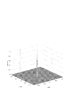
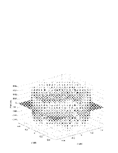
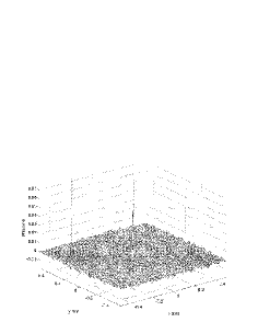
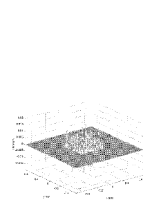
Fig. 3: Numerical experiment of the one-step time reversal procedure. Top Left: initial condition $p(0,{\bf x})$, a peaked Gaussian of maximal amplitude equal to $1$. Top Right: forward solution $p(T^{-},{\bf x})$, of maximal amplitude $0.04$. Bottom Right: recorded solution $p(T^{+},{\bf x})$, of maximal amplitude $0.015$ on the domain $\Omega=(-1/6,1/6)^{2}$. Bottom Left: back-propagated solution $p(2T,{\bf x})$, of maximal amplitude $0.07$.

In the numerical simulations, there is no blurring, $f({\bf x})=\delta({\bf x})$, and the array of receivers is the domain $\Omega=(-1/6,1/6)^{2}$ ($\chi({\bf x})$ is the characteristic function of $\Omega$). Note that the truncated signal does not retain any information about the ballistic part (the part that propagates without scattering with the underlying medium). In homogeneous medium, the truncated signal would then be identically zero and no refocusing would be observed. The interesting aspect of time reversal is that a coherent signal emerges at time $2T$ out of a signal at time $T^{+}$ that seems to have no useful information.

3 Theory of Time Reversal in Random Media

Our objective is now to present a theory that explains in a quantitative manner the refocusing properties described in the preceding sections. We consider here the one-step time reversal for acoustic wave. Generalizations to other types of waves and more general processings in (9) are given in section 4.

3.1 Refocused Signal

We recall that the one-step time reversal procedure consists of letting an initial pulse ${\bf S}({\bf x})$ propagate according to (4) until time $T$,

$${\bf u}(T^{-},{\bf x})=\displaystyle\int_{\mathbb{R}^{3}}G(T,{\bf x};{\bf z}){\bf S}({\bf z})d{\bf z},$$

where $G(T,{\bf x};{\bf z})$ is the Green’s matrix solution of

$$\!\!\!A({\bf x})\dfrac{\partial{G(t,{\bf x};{\bf y})}}{\partial{t}}+D^{j}\dfrac{\partial{G(t,{\bf x};{\bf y})}}{\partial{x^{j}}}=0,~{}0\leq t\leq T$$ (11)

$$\!\!\!G(0,{\bf x};{\bf y})=I\delta({\bf x}-{\bf y}).$$

At time $T$, the “intelligent” array reverses the signal. For acoustic pulses, this means keeping pressure unchanged and reversing the sign of the velocity field. The array of receivers is located in $\Omega\subset\mathbb{R}^{3}$. The amplification function $\chi({\bf x})$ is an arbitrary bounded function supported in $\Omega$, such as its characteristic function ($\chi({\bf x})=1$ for ${\bf x}\in\Omega$ and $\chi({\bf x})=0$ otherwise) when all transducers have the same amplification factor. We also allow for some blurring of the recorded data modeled by a convolution with a function $f({\bf x})$. The case $f({\bf x})=\delta({\bf x})$ corresponds to exact measurements. Finally, the signal is time reversed, that is, the direction of the acoustic velocity is reversed. Here, the operator $\Gamma$ in (8) is simply multiplication by the matrix

$$\Gamma=\mbox{Diag}(-1,-1,-1,1).$$ (12)

The signal at time $T^{+}$ after time reversal takes then the form

$${\bf u}(T^{+},{\bf x})=\displaystyle\int_{\mathbb{R}^{6}}\Gamma G(T,{\bf y}^{\prime};{\bf z})\chi({\bf x})\chi({\bf y}^{\prime})f({\bf x}-{\bf y}^{\prime}){\bf S}({\bf z})d{\bf z}d{\bf y}^{\prime}.$$ (13)

The last step (9) consists of letting the time reversed field propagate through the random medium until time $2T$. To compare this signal with the initial pulse ${\bf S}$, we need to reverse the acoustic velocity once again, and define

$${\bf u}^{B}({\bf x})=\Gamma{\bf u}(2T,{\bf x})=\displaystyle\int_{\mathbb{R}^{9}}\Gamma G(T,{\bf x};{\bf y})\Gamma G(T,{\bf y}^{\prime};{\bf z})\chi({\bf y})\chi({\bf y}^{\prime})f({\bf y}-{\bf y}^{\prime}){\bf S}({\bf z})d{\bf y}d{\bf y}^{\prime}d{\bf z}.$$ (14)

The time reversibility of first-order hyperbolic systems implies that ${\bf u}^{B}({\bf x})={\bf S}({\bf x})$ when $\Omega=\mathbb{R}^{3}$, $\chi\equiv 1$, and $f({\bf x})=\delta({\bf x})$, that is, when full and non-distorted measurements are available. It remains to understand which features of ${\bf S}$ are retained by ${\bf u}^{B}({\bf x})$ when only partial measurement is available.

3.2 Localized Source and Scaling

We consider an asymptotic solution of the time reversal problem (4), (9) when the support $\lambda$ of the initial pulse ${\bf S}({\bf x})$ is much smaller than the distance $L$ of propagation between the source and the recording array: $\varepsilon=\lambda/L\ll 1$. We also take the size $a$ of the array comparable to $L$: $a/L=O(1)$. We assume that the time $T$ between the emission of the original signal and recording is of order $L/c_{0}$, where $c_{0}$ is a typical speed of propagation of the acoustic wave. We consequently consider the initial pulse to be of the form

$${\bf u}(0,{\bf x})={\bf S}(\dfrac{{\bf x}-{\bf x}_{0}}{\varepsilon})$$

in non-dimensionalized variables ${\bf x}^{\prime}={\bf x}/L$ and $t^{\prime}=t/(L/c_{0})$. We drop primes to simplify notation. Here ${\bf x}_{0}$ is the location of the source. The transducers obviously have to be capable of capturing signals of frequency $\varepsilon^{-1}$ and blurring should happen on the scale of the source, so we replace $f({\bf x})$ by $\varepsilon^{-3}f(\varepsilon^{-1}{\bf x})$. Finally, we are interested in the refocusing properties of ${\bf u}^{B}({\bf x})$ in the vicinity of ${\bf x}_{0}$. We therefore introduce the scaling ${\bf x}={\bf x}_{0}+\varepsilon\boldsymbol{\xi}$. With these changes of variables, expression (14) is recast as

$${\bf u}^{B}(\boldsymbol{\xi};{\bf x}_{0})=\Gamma{\bf u}(2T,{\bf x}_{0}+\varepsilon\boldsymbol{\xi})$$ (15)

$$~{}~{}~{}~{}~{}~{}~{}~{}~{}~{}~{}~{}=\displaystyle\int_{\mathbb{R}^{9}}\Gamma G(T,{\bf x}_{0}+\varepsilon\boldsymbol{\xi};{\bf y})\Gamma G(T,{\bf y}^{\prime};{\bf x}_{0}+\varepsilon{\bf z})\chi({\bf y},{\bf y}^{\prime}){\bf S}({\bf z})d{\bf y}d{\bf y}^{\prime}d{\bf z},$$

where

$$\chi({\bf y},{\bf y}^{\prime})=\chi({\bf y})\chi({\bf y}^{\prime})f(\dfrac{{\bf y}-{\bf y}^{\prime}}{\varepsilon}).$$ (16)

In the sequel we will also allow the medium to vary on a scale comparable to the source scale $\varepsilon$. Thus the Green’s function $G$ and the matrix $A$ depend on $\varepsilon$. We do not make this dependence explicit to simplify notation. We are interested in the limit of ${\bf u}^{B}(\boldsymbol{\xi};{\bf x}_{0})$ as $\varepsilon\to 0$. The scaling considered here is well adapted both to the physical experiments in [7] and the numerical experiments in Fig. 3.

3.3 Adjoint Green’s Function

The analysis of the re-propagated signal relies on the study of the two point correlation at nearby points of the Green’s matrix in (15). There are two undesirable features in (15). First, the two nearby points ${\bf x}_{0}+\varepsilon\boldsymbol{\xi}$ and ${\bf x}_{0}+\varepsilon{\bf z}$ are terminal and initial points in their respective Green’s matrices. Second, one would like the matrix $\Gamma$ between the two Green’s matrices to be outside of their product. However, $\Gamma$ and $G$ do not commute. For these reasons, we introduce the adjoint Green’s matrix, solution of

$$\begin{array}[]{l}\dfrac{\partial{G_{*}(t,{\bf x};{\bf y})}}{\partial{t}}A({\bf x})+\dfrac{\partial{G_{*}(t,{\bf x};{\bf y})}}{\partial{x^{j}}}D^{j}=0\\ G_{*}(0,{\bf x};{\bf y})=A^{-1}({\bf x})\delta({\bf x}-{\bf y}).\end{array}$$ (17)

We now prove that

$$G_{*}(t,{\bf x};{\bf y})=\Gamma G(t,{\bf y};{\bf x})A^{-1}({\bf x})\Gamma.$$ (18)

Note that for all initial data ${\bf S}({\bf x})$, the solution ${\bf u}(t,{\bf x})$ of (4) satisfies

$${\bf u}(t,{\bf x})=\displaystyle\int_{\mathbb{R}^{3}}G(t-s,{\bf x};{\bf y}){\bf u}(s,{\bf y})d{\bf y}$$

for all $0\leq s\leq t\leq T$ since the coefficients in (4) are time-independent. Differentiating the above with respect to $s$ and using (4) yields

$$0=\displaystyle\int_{\mathbb{R}^{3}}\Big{(}-\dfrac{\partial{G(t-s,{\bf x};{\bf y})}}{\partial{t}}{\bf u}(s,{\bf y})-G(t-s,{\bf x};{\bf y})A^{-1}({\bf y})D^{j}\dfrac{\partial{{\bf u}(s,{\bf y})}}{\partial{y^{j}}}\Big{)}d{\bf y}$$

Upon integrating by parts and letting $s=0$, we get

$$0=\displaystyle\int_{\mathbb{R}^{3}}\Big{(}-\dfrac{\partial{G(t,{\bf x};{\bf y})}}{\partial{t}}+\dfrac{\partial{}}{\partial{y^{j}}}\left[G(t,{\bf x};{\bf y})A^{-1}({\bf y})D^{j}\right]\Big{)}{\bf S}({\bf y})d{\bf y}.$$

Since the above relation holds for all test functions ${\bf S}({\bf y})$, we deduce that

$$\dfrac{\partial{G(t,{\bf x};{\bf y})}}{\partial{t}}-\dfrac{\partial{}}{\partial{y^{j}}}\left[G(t,{\bf x};{\bf y})A^{-1}({\bf y})D^{j}\right]=0.$$ (19)

Interchanging ${\bf x}$ and ${\bf y}$ in the above equation and multiplying it on the left and the right by $\Gamma$, we obtain that

$$\dfrac{\partial{}}{\partial{t}}\left[\Gamma G(t,{\bf y};{\bf x})A^{-1}({\bf x})\right]A({\bf x})\Gamma-\dfrac{\partial{}}{\partial{x^{j}}}\left[\Gamma G(t,{\bf y};{\bf x})A^{-1}({\bf x})\right]D^{j}\Gamma=0.$$ (20)

We remark that

$$\Gamma D^{j}=-D^{j}\Gamma\qquad\mbox{ and }\qquad\Gamma A({\bf x})=A({\bf x})\Gamma,$$ (21)

so that

$$\dfrac{\partial{}}{\partial{t}}\left[\Gamma G(t,{\bf y};{\bf x})A^{-1}({\bf x})\Gamma\right]A({\bf x})+\dfrac{\partial{}}{\partial{x^{j}}}\left[\Gamma G(t,{\bf y};{\bf x})A^{-1}({\bf x})\Gamma\right]D^{j}=0$$

with $\Gamma G(0,{\bf y};{\bf x})A^{-1}({\bf x})\Gamma=A^{-1}({\bf x})\delta({\bf x}-{\bf y})$. Thus (18) follows from the uniqueness of the solution to the above hyperbolic system with given initial conditions. We can now recast (15) as

$$\begin{array}[]{ll}{\bf u}^{B}(\boldsymbol{\xi};{\bf x}_{0})\,=\,\displaystyle\int_{\mathbb{R}^{9}}&\!\!\!\Gamma G(T,{\bf x}_{0}+\varepsilon\boldsymbol{\xi};{\bf y})G_{*}(T,{\bf x}_{0}+\varepsilon{\bf z};{\bf y}^{\prime})\Gamma\\ &\!\!\!\times\chi({\bf y})\chi({\bf y}^{\prime})f(\dfrac{{\bf y}-{\bf y}^{\prime}}{\varepsilon})A({\bf x}_{0}+\varepsilon{\bf z}){\bf S}({\bf z})d{\bf y}d{\bf y}^{\prime}d{\bf z}.\end{array}$$ (24)

One further simplifies (24) with the help of the auxiliary matrix-valued functions $Q(t,{\bf x};{\bf q})$ and $Q_{*}(t,{\bf x},{\bf q})$ defined by

$$\begin{array}[]{rcl}Q(T,{\bf x};{\bf q})&=&\displaystyle\int_{\mathbb{R}^{3}}G(T,{\bf x};{\bf y})\chi({\bf y})e^{i{\bf q}\cdot{\bf y}/\varepsilon}d{\bf y},\\ Q_{*}(T,{\bf x};{\bf q})&=&\displaystyle\int_{\mathbb{R}^{3}}G_{*}(T,{\bf x};{\bf y})\chi({\bf y})e^{-i{\bf q}\cdot{\bf y}/\varepsilon}d{\bf y}.\end{array}$$ (25)

They solve the hyperbolic equations (4) and (17) with initial conditions given by $Q(0,{\bf x};{\bf q})=\chi({\bf x})e^{i{\bf q}\cdot{\bf x}/\varepsilon}I$ and $Q_{*}(0,{\bf x};{\bf q})=A^{-1}({\bf x})\chi({\bf x})e^{-i{\bf q}\cdot{\bf x}/\varepsilon}$, respectively. Thus (24) becomes

$${\bf u}^{B}(\boldsymbol{\xi};{\bf x}_{0})\!\!=\!\!\displaystyle\int_{\mathbb{R}^{6}}\!\!\Gamma Q(T,{\bf x}_{0}+\varepsilon\boldsymbol{\xi};{\bf q})Q_{*}(T,{\bf x}_{0}+\varepsilon{\bf z};{\bf q})\Gamma A({\bf x}_{0}+\varepsilon{\bf z}){\bf S}({\bf z})\hat{f}({\bf q})\frac{d{\bf q}d{\bf z}}{(2\pi)^{3}},$$ (26)

where $\hat{f}({\bf q})=\int_{\mathbb{R}^{3}}e^{-i{\bf q}\cdot{\bf x}}f({\bf x})d{\bf x}$ is the Fourier transform of $f({\bf x})$.

3.4 Wigner Transform

The back-propagated signal in (26) now has the suitable form to be analyzed in the Wigner transform formalism [14, 24]. We define

$$W_{\varepsilon}(t,{\bf x},{\bf k})=\displaystyle\int_{\mathbb{R}^{3}}\hat{f}({\bf q})U_{\varepsilon}(t,{\bf x},{\bf k};{\bf q}){d{\bf q}},$$ (27)

where

$$U_{\varepsilon}(t,{\bf x},{\bf k};{\bf q})=\displaystyle\int_{\mathbb{R}^{3}}e^{i{\bf k}\cdot{\bf y}}Q(t,{\bf x}-\dfrac{\varepsilon{\bf y}}{2};{\bf q})Q_{*}(t,{\bf x}+\dfrac{\varepsilon{\bf y}}{2};{\bf q})\dfrac{d{\bf y}}{(2\pi)^{3}}.$$ (28)

Taking inverse Fourier transform we verify that

$$Q(t,{\bf x};{\bf q})Q_{*}(t,{\bf y};{\bf q})=\displaystyle\int_{\mathbb{R}^{3}}e^{-i{\bf k}\cdot({\bf y}-{\bf x})/\varepsilon}U_{\varepsilon}(t,\dfrac{{\bf x}+{\bf y}}{2},{\bf k};{\bf q})d{\bf k},$$

hence

$${\bf u}^{B}(\boldsymbol{\xi};{\bf x}_{0})=\displaystyle\int_{\mathbb{R}^{6}}e^{i{\bf k}\cdot(\boldsymbol{\xi}-{\bf z})}\Gamma W_{\varepsilon}(T,{\bf x}_{0}+\varepsilon\dfrac{{\bf z}+\boldsymbol{\xi}}{2},{\bf k})\Gamma A({\bf x}_{0}+\varepsilon{\bf z}){\bf S}({\bf z})\frac{d{\bf z}d{\bf k}}{(2\pi)^{3}}.$$ (29)

We have thus reduced the analysis of ${\bf u}(\boldsymbol{\xi};{\bf x}_{0})$ as $\varepsilon\to 0$ to that of the asymptotic properties of the Wigner transform $W_{\varepsilon}$. The Wigner transform has been used extensively in the study of wave propagation in random media, especially in the derivation of radiative transport equations modeling the propagation of high frequency waves. We refer to [14, 21, 24]. Note that in the usual definition of the Wigner transform, one has the adjoint matrix $Q^{*}$ in place of $Q_{*}$ in (28). This difference is not essential since $Q_{*}$ and $Q^{*}$ satisfy the same evolution equation, though with different initial data.

The main reason for using the Wigner transform in (29) is that $W_{\varepsilon}$ has a weak limit $W$ as $\varepsilon\to 0$. Its existence follows from simple a priori bounds for $W_{\varepsilon}(t,{\bf x},{\bf k})$. Let us introduce the space ${\cal A}$ of matrix-valued functions $\phi({\bf x},{\bf k})$ bounded in the norm $\|\cdot\|_{{\cal A}}$ defined by

$$\|\phi\|_{{\cal A}}=\displaystyle\int_{\mathbb{R}^{3}}\sup_{{\bf x}}\|\tilde{\phi}({\bf x},{\bf y})\|d{\bf y},\qquad\mbox{ where }\quad\tilde{\phi}({\bf x},{\bf y})=\displaystyle\int_{\mathbb{R}^{3}}e^{-i{\bf k}\cdot{\bf y}}\phi({\bf x},{\bf k})d{\bf k}.$$

We denote by ${\cal A}^{\prime}$ its dual space, which is a space of distributions large enough to contain matrix-valued bounded measures, for instance. We then have the following result:

Lemma 1.

Let $\chi({\bf x})\in L^{2}(\mathbb{R}^{3})$ and $\hat{f}({\bf q})\in L^{1}(\mathbb{R}^{3})$. Then there is a constant $C>0$ independent of $\varepsilon>0$ and $t\in[0,\infty)$ such that for all $t\in[0,\infty)$, we have $\|W_{\varepsilon}(t,{\bf x},{\bf k})\|_{{\cal A}^{\prime}}<C$.

The proof of this lemma is essentially contained in [14, 21]; see also [1]. One may actually get $L^{2}$-bounds for $W_{\varepsilon}$ in our setting because of the regularizing effect of $\hat{f}$ in (27) but this is not essential for the purposes of this paper. We therefore obtain the existence of a subsequence $\varepsilon_{k}\to 0$ such that $W_{\varepsilon_{k}}$ converges weakly to a distribution $W\in{\cal A}^{\prime}$. Moreover, an easy calculation shows that at time $t=0$, we have

$$W(0,{\bf x}_{0},{\bf k})=|\chi({\bf x}_{0})|^{2}A_{0}^{-1}({\bf x}_{0})\hat{f}({\bf k}).$$ (30)

Here, $A_{0}=A$ when $A$ is independent of $\varepsilon$, and $A_{0}=\lim\limits_{\varepsilon\to 0}A_{\varepsilon}$ if we assume that the family of matrices $A_{\varepsilon}({\bf x})$ is uniformly bounded and continuous with the limit $A_{0}$ in ${\cal C}({\mathbb{R}}^{d})$. These assumptions on $A_{\varepsilon}$ are sufficient to deal with the radiative transport regime we will consider in section 3.7. Under the same assumptions on $A_{\varepsilon}$, we have the following result.

Proposition 2.

The back-propagated signal ${\bf u}^{B}(\boldsymbol{\xi};{\bf x}_{0})$ given by (29) converges weakly in ${\cal S}^{\prime}(\mathbb{R}^{3}\times\mathbb{R}^{3})$ as $\varepsilon\to 0$ to the limit

$${\bf u}^{B}(\boldsymbol{\xi};{\bf x}_{0})=\displaystyle\int_{\mathbb{R}^{6}}e^{i{\bf k}\cdot(\boldsymbol{\xi}-{\bf z})}\Gamma W(T,{\bf x}_{0},{\bf k})\Gamma A_{0}({\bf x}_{0}){\bf S}({\bf z})\frac{d{\bf z}d{\bf k}}{(2\pi)^{3}}.$$ (31)

The proof of this proposition is based on taking the duality product of ${\bf u}^{B}(\boldsymbol{\xi};{\bf x}_{0})$ with a vector-valued test function $\boldsymbol{\phi}(\boldsymbol{\xi};{\bf x}_{0})$ in ${\cal S}(\mathbb{R}^{3}\times\mathbb{R}^{3})$. After a change of variables we obtain $\langle{\bf u}^{B},\boldsymbol{\phi}\rangle=\langle W_{\varepsilon},Z_{\varepsilon}\rangle.$ Here the duality product for matrices is given by the trace $\langle A,B\rangle=\sum_{i,k}\langle A_{ik},B_{ik}\rangle$, and

$$Z_{\varepsilon}({\bf x}_{0},{\bf k})=\displaystyle\int_{\mathbb{R}^{6}}e^{i{\bf k}\cdot({\bf z}-\boldsymbol{\xi})}\Gamma\boldsymbol{\phi}(\boldsymbol{\xi},{\bf x}_{0}-\varepsilon\dfrac{{\bf z}+\boldsymbol{\xi}}{2}){\bf S}^{*}({\bf z})A_{\varepsilon}({\bf x}_{0}+\varepsilon\dfrac{{\bf z}-\boldsymbol{\xi}}{2})\Gamma\frac{d{\bf z}d\boldsymbol{\xi}}{(2\pi)^{3}}.$$ (32)

Defining $Z$ as the limit of $Z_{\varepsilon}$ as $\varepsilon\to 0$ by replacing formally $\varepsilon$ by $0$ in the above expression, (31) follows from showing that $\|Z_{\varepsilon}-Z\|_{{\cal A}}\to 0$ as $\varepsilon\to 0$. This is straightforward and we omit the details.

The above proposition tells us how to reconstruct the back-propagated solution in the high frequency limit from the limit Wigner matrix $W$. Notice that we have made almost no assumptions on the medium described by the matrix $A_{\varepsilon}({\bf x})$. At this level, the medium can be either homogeneous or heterogeneous. Without any further assumptions, we can also obtain some information about the matrix $W$. Let us define the dispersion matrix for the system (4) as [24]

$$L({\bf x},{\bf k})=A_{0}^{-1}({\bf x})k_{j}D^{j}.$$ (33)

It is given explicitly by

$$L({\bf x},{\bf k})=\left(\begin{matrix}0&0&0&k_{1}/\rho({\bf x})\cr 0&0&0&k_{2}/\rho({\bf x})\cr 0&0&0&k_{3}/\rho({\bf x})\cr k_{1}/\kappa({\bf x})&k_{2}/\kappa({\bf x})&k_{3}/\kappa({\bf x})&0\cr\end{matrix}\right).$$

The matrix $L$ has a double eigenvalue $\omega_{0}=0$ and two simple eigenvalues $\omega_{\pm}({\bf x},{\bf k})=\pm c({\bf x})|{\bf k}|$, where $c({\bf x})=1/\sqrt{\rho({\bf x})\kappa({\bf x})}$ is the speed of sound. The eigenvalues $\omega_{\pm}$ are associated with eigenvectors ${\bf b}_{\pm}({\bf x},{\bf k})$ and the eigenvalue $\omega_{0}=0$ is associated with the eigenvectors ${\bf b}_{j}({\bf x},{\bf k})$, $j=1,2$. They are given by

$${\bf b}_{\pm}({\bf x},{\bf k})=\left(\begin{array}[]{c}\pm\dfrac{\hat{\bf k}}{\sqrt{2\rho({\bf x})}}\\ \dfrac{1}{\sqrt{2\kappa({\bf x})}}\end{array}\right),\qquad\qquad{\bf b}_{j}({\bf x},{\bf k})=\left(\begin{array}[]{c}\dfrac{{\bf z}^{j}({\bf k})}{\sqrt{\rho({\bf x})}}\\ 0\end{array}\right),$$ (34)

where $\hat{\bf k}={\bf k}/|{\bf k}|$ and ${\bf z}^{1}({\bf k})$ and ${\bf z}^{2}({\bf k})$ are chosen so that the triple $({\hat{\bf k}},{\bf z}^{1}({\bf k}),{\bf z}^{2}({\bf k}))$ forms an orthonormal basis. The eigenvectors are normalized so that

$$(A_{0}({\bf x}){\bf b}_{j}({\bf x},{\bf k})\cdot{\bf b}_{k}({\bf x},{\bf k}))=\delta_{jk},$$ (35)

for all $j,k\in J=\{+,-,1,2\}$. The space of $4\times 4$ matrices is clearly spanned by the basis ${\bf b}_{j}\otimes{\bf b}_{k}$. We then have the following result:

Proposition 3.

There exist scalar distributions $a_{\pm}$ and $a_{0}^{mn}$, $m,n=1,2$ so that the limit Wigner distribution matrix can be decomposed as

$$W(t,{\bf x},{\bf k})=\displaystyle\sum_{j,m=1}^{2}a_{0}^{jm}(t,{\bf x},{\bf k}){\bf b}_{j}({\bf x},{\bf k})\otimes{\bf b}_{m}({\bf x},{\bf k})$$ (36)

$$\quad+\,a_{+}(t,{\bf x},{\bf k}){\bf b}_{+}({\bf x},{\bf k})\otimes{\bf b}_{+}({\bf x},{\bf k})+a_{-}(t,{\bf x},{\bf k}){\bf b}_{-}({\bf x},{\bf k})\otimes{\bf b}_{-}({\bf x},{\bf k}).$$

The main result of this proposition is that the cross terms ${\bf b}_{j}\otimes{\bf b}_{k}$ with $\omega_{j}\not=\omega_{k}$ do not contribute to the limit $W$. The proof of this proposition can be found in [14] and a formal derivation in [24].

The initial conditions for the amplitudes $a_{j}$ are calculated using the identity

$$A_{0}^{-1}({\bf x})=\displaystyle\sum_{j\in J}{\bf b}_{j}({\bf x},{\bf k})\otimes{\bf b}_{j}({\bf x},{\bf k}).$$

Then (30) implies that $a_{0}^{12}(0,{\bf x},{\bf k})=a_{0}^{21}(0,{\bf x},{\bf k})=0$ and

$$a_{0}^{jj}(0,{\bf x},{\bf k})=a_{\pm}(0,{\bf x},{\bf k})=|\chi({\bf x})|^{2}f({\bf k}),~{}~{}j=1,2.$$ (37)

3.5 Mode Decomposition and Refocusing

We can use the above result to recast (31) as

$${\bf u}^{B}(\boldsymbol{\xi};{\bf x}_{0})=(F(T,\cdot;{\bf x}_{0})*{\bf S})(\boldsymbol{\xi}),$$ (38)

where

$$F(T,\boldsymbol{\xi};{\bf x}_{0})=\displaystyle\sum_{m,n=1}^{2}\displaystyle\int_{\mathbb{R}^{3}}e^{i{\bf k}\cdot\boldsymbol{\xi}}a_{0}^{mn}(T,{\bf x}_{0};{\bf k})\Gamma{\bf b}_{m}({\bf x}_{0},{\bf k})\otimes{\bf b}_{n}({\bf x}_{0},{\bf k})A_{0}({\bf x}_{0})\Gamma\frac{d{\bf k}}{(2\pi)^{3}}$$

$$~{}~{}~{}~{}~{}~{}~{}~{}~{}~{}~{}~{}~{}~{}~{}+\displaystyle\int_{\mathbb{R}^{3}}e^{i{\bf k}\cdot\boldsymbol{\xi}}a_{+}(T,{\bf x}_{0};{\bf k})\Gamma{\bf b}_{+}({\bf x}_{0},{\bf k})\otimes{\bf b}_{+}({\bf x}_{0},{\bf k})A_{0}({\bf x}_{0})\Gamma\frac{d{\bf k}}{(2\pi)^{3}}$$ (39)

$$~{}~{}~{}~{}~{}~{}~{}~{}~{}~{}~{}~{}~{}~{}~{}+\displaystyle\int_{\mathbb{R}^{3}}e^{i{\bf k}\cdot\boldsymbol{\xi}}a_{-}(T,{\bf x}_{0};{\bf k})\Gamma{\bf b}_{-}({\bf x}_{0},{\bf k})\otimes{\bf b}_{-}({\bf x}_{0},{\bf k})A_{0}({\bf x}_{0})\Gamma\frac{d{\bf k}}{(2\pi)^{3}}.$$

This expression can be used to assess the quality of the refocusing. When $F(T,\boldsymbol{\xi};{\bf x}_{0})$ has a narrow support in $\boldsymbol{\xi}$, refocusing is good. When its support in $\boldsymbol{\xi}$ grows larger, its quality degrades. The spatial decay of the kernel $F(t,\boldsymbol{\xi};{\bf x}_{0})$ in $\boldsymbol{\xi}$ is directly related to the smoothness in ${\bf k}$ of its Fourier transform in $\boldsymbol{\xi}$:

$$\hat{F}(T,{\bf k};{\bf x}_{0})=\displaystyle\sum_{m,n=1}^{2}a_{0}^{mn}(T,{\bf x}_{0};{\bf k})\Gamma{\bf b}_{m}({\bf x}_{0},{\bf k})\otimes{\bf b}_{n}({\bf x}_{0},{\bf k})A_{0}({\bf x}_{0})\Gamma\frac{d{\bf k}}{(2\pi)^{3}}$$

$$+\Gamma\left[a_{+}(T,{\bf x}_{0};{\bf k}){\bf b}_{+}({\bf x}_{0},{\bf k})\otimes{\bf b}_{+}({\bf x}_{0},{\bf k})\!+a_{-}(T,{\bf x}_{0};{\bf k}){\bf b}_{-}({\bf x}_{0},{\bf k})\otimes{\bf b}_{-}({\bf x}_{0},{\bf k})\right]A_{0}({\bf x}_{0})\Gamma.$$

Namely, for $F$ to decay in $\boldsymbol{\xi}$, one needs $\hat{F}({\bf k})$ to be smooth in ${\bf k}$. However, the eigenvectors ${\bf b}_{j}$ are singular at ${\bf k}=0$ as can be seen from the explicit expressions (34). Therefore, $\hat{F}$ a priori is not smooth at ${\bf k}=0$. This means that in order to obtain good refocusing one needs the original signal to have no low frequencies: $\hat{S}({\bf k})=0$ near ${\bf k}=0$. Low frequencies in the initial data will not refocus well.

We can further simplify (38)-(39) is we assume that the initial source is irrotational. Taking Fourier transform of both sides in (38), we obtain that

$$\hat{\bf u}^{B}({\bf k};{\bf x}_{0})=\displaystyle\sum_{j,n\in J}a_{j}(T,{\bf x}_{0},{\bf k})\hat{S}_{n}({\bf k})(A_{0}({\bf x}_{0})\Gamma{\bf b}_{n}({\bf x}_{0},{\bf k})\cdot{\bf b}_{j}({\bf x}_{0},{\bf k}))\Gamma{\bf b}_{j}({\bf x}_{0},{\bf k})$$ (40)

where we have defined

$$\hat{\bf S}({\bf k})=\displaystyle\sum_{n\in J}\hat{S}_{n}({\bf k}){\bf b}_{n}({\bf x}_{0},{\bf k}).$$ (41)

Irrotationality of the initial source means that $\hat{S}_{1}$ and $\hat{S}_{2}$ identically vanish, or equivalently that

$${\bf S}({\bf x})=\left(\begin{matrix}\nabla\phi({\bf x})\cr p({\bf x})\cr\end{matrix}\right)$$ (42)

for some pressure $p({\bf x})$ and potential $\phi({\bf x})$. Remarking that $\Gamma{\bf b}_{\pm}=-{\bf b}_{\mp}$ and by irrotationality that $(A_{0}({\bf x}_{0})\hat{\bf S}({\bf k})\cdot{\bf b}_{1,2}({\bf k}))=0$, we use (35) to recast (40) as

$$\hat{\bf u}^{B}({\bf k};{\bf x}_{0})=a_{-}(T,{\bf x}_{0},{\bf k})\hat{S}_{+}({\bf k}){\bf b}_{+}({\bf x}_{0},{\bf k})+a_{+}(T,{\bf x}_{0},{\bf k})\hat{S}_{-}({\bf k}){\bf b}_{-}({\bf x}_{0},{\bf k}).$$ (43)

Decomposing the source ${\bf S}({\bf x})$ as

$${\bf S}({\bf x})={\bf S}_{+}({\bf x})+{\bf S}_{-}({\bf x}),\qquad\mbox{such that}\quad\hat{\bf S}_{\pm}({\bf k})=\hat{S}_{\pm}({\bf k}){\bf b}_{\pm}({\bf x}_{0},{\bf k}),$$

the back-propagated signal takes the form

$${\bf u}^{B}(\boldsymbol{\xi};{\bf x}_{0})=(\hat{a}_{-}(T,{\bf x}_{0},\cdot)*{\bf S}_{+}(\cdot))(\boldsymbol{\xi})+(\hat{a}_{+}(T,{\bf x}_{0},\cdot)*{\bf S}_{-}(\cdot))(\boldsymbol{\xi})$$ (44)

where $\hat{a}_{\pm}$ is the Fourier of $a_{\pm}$ in ${\bf k}$. This form is much more tractable than (38)-(39). It is also almost as general. Indeed, rotational modes do not propagate in the high frequency regime. Therefore, they are exactly back-propagated when $\chi({\bf x}_{0})=1$ and $f({\bf x})=\delta({\bf x})$, and not back-propagated at all when $\chi({\bf x}_{0})=0$. All the refocusing properties are thus captured by the amplitudes $a_{\pm}(T,{\bf x}_{0},{\bf k})$. Their evolution equation characterizes how waves propagate in the medium and their initial conditions characterize the recording array.

3.6 Homogeneous Media

In homogeneous media with $c({\bf x})=c_{0}$ the amplitudes $a_{\pm}(T,{\bf x},{\bf k})$ satisfy the free transport equation [14, 24]

$$\dfrac{\partial{a_{\pm}}}{\partial{t}}\pm c_{0}{\hat{\bf k}}\cdot\nabla_{\bf x}a_{\pm}=0$$ (45)

with initial data $a_{\pm}(0,{\bf x},{\bf k})=|\chi({\bf x})|^{2}f({\bf k})$ as in (37). They are therefore given by

$$a_{\pm}(t,{\bf x}_{0},{\bf k})=|\chi({\bf x}_{0}\mp c_{0}\hat{\bf k}t)|^{2}\hat{f}({\bf k}).$$ (46)

These amplitudes become more and more singular in ${\bf k}$ as time grows since their gradient in ${\bf k}$ grows linearly with time. The corresponding kernel $F=F_{H}$ decays therefore more slowly in $\boldsymbol{\xi}$ as time grows. This implies that the quality of the refocusing degrades with time. For sufficiently large times, all the energy has left the domain $\Omega$ (assumed to be bounded), and the coefficients $a_{\pm}(t,{\bf x}_{0},{\bf k})$ vanish. Therefore the back-propagated signal ${\bf u}^{B}(\boldsymbol{\xi};{\bf x}_{0})$ also vanishes, which means that there is no refocusing at all. The same conclusions could also be drawn by analyzing (14) directly in a homogeneous medium. This is the situation in the numerical experiment presented in Fig. 3: in a homogeneous medium, the back-propagated signal would vanish.

3.7 Heterogeneous Media and Radiative Transport Regime

The results of the preceding sections show how the back-propagated signal ${\bf u}^{B}(\boldsymbol{\xi};{\bf x}_{0})$ is related to the propagating modes $a_{\pm}(T,{\bf x}_{0},{\bf k})$ of the Wigner matrix $W(T,{\bf x}_{0},{\bf k})$. The form assumed by the modes $a_{\pm}(T,{\bf x}_{0},{\bf k})$, and in particular their smoothness in ${\bf k}$, will depend on the hypotheses we make on the underlying medium; i.e., on the density $\rho({\bf x})$ and compressibility $\kappa({\bf x})$ that appear in the matrix $A({\bf x})$. We have seen that partial measurements in homogeneous media yield poor refocusing properties. We now show that refocusing is much better in random media.

We consider here the radiative transport regime, also known as weak coupling limit. There, the fluctuations in the physical parameters are weak and vary on a scale comparable to the scale of the initial source. Density and compressibility assume the form

$$\rho({\bf x})=\rho_{0}+\sqrt{\varepsilon}\rho_{1}(\dfrac{{\bf x}}{\varepsilon})\qquad\mbox{ and }\qquad\kappa({\bf x})=\kappa_{0}+\sqrt{\varepsilon}\kappa_{1}(\dfrac{{\bf x}}{\varepsilon}).$$ (47)

The functions $\rho_{1}$ and $\kappa_{1}$ are assumed to be mean-zero spatially homogeneous processes. The average (with respect to realizations of the medium) of the propagating amplitudes $a_{\pm}$, denoted by $\bar{a}_{\pm}$, satisfy in the high frequency limit $\varepsilon\to 0$ a radiative transfer equation (RTE), which is a linear Boltzmann equation of the form

$$\begin{array}[]{l}\dfrac{\partial{\bar{a}_{\pm}}}{\partial{t}}\pm c_{0}\hat{\bf k}\cdot\nabla_{\bf x}\bar{a}_{\pm}=\displaystyle\int_{\mathbb{R}^{3}}\sigma({\bf k},{\bf p})(\bar{a}_{\pm}(t,{\bf x},{\bf p})-\bar{a}_{\pm}(t,{\bf x},{\bf k}))\delta(c_{0}(|{\bf k}|-|{\bf p}|))d{\bf p}\\ \bar{a}_{\pm}(0,{\bf x},{\bf k})=|\chi({\bf x})|^{2}\hat{f}({\bf k}).\end{array}\!\!$$ (48)

The scattering coefficient $\sigma({\bf k},{\bf p})$ depends on the power spectra of $\rho_{1}$ and $\kappa_{1}$. We refer to [24] for the details of the derivation and explicit form of $\sigma({\bf k},{\bf p})$. The above result remains formal for the wave equation and requires to average over the realizations of the random medium although this is not necessary in the physical and numerical time reversal experiments. A rigorous proof of the derivation of the linear Boltzmann equation (which also requires to average over realizations) has only been obtained for the Schrödinger equation; see [9, 26]. Nevertheless, the above result formally characterizes the filter $F(T,\boldsymbol{\xi};{\bf x}_{0})$ introduced in (39) and (44).

The transport equation (48) has a smoothing effect best seen in its integral formulation. Let us define the total scattering coefficient $\Sigma({\bf k})=\int_{\mathbb{R}^{3}}\sigma({\bf k},{\bf p})\delta(c_{0}(|{\bf k}|-|{\bf p}|))d{\bf p}$. Then the transport equation (48) may be rewritten as

$$\bar{a}_{\pm}(t,{\bf x},{\bf k})=\bar{a}_{\pm}(0,{\bf x}\mp c_{0}{\hat{\bf k}}t,{\bf k})e^{-\Sigma({\bf k})t}$$ (49)

$$+\frac{|{\bf k}|^{2}}{c_{0}}\int_{0}^{t}ds\displaystyle\int_{S^{2}}\sigma({\bf k},|{\bf k}|{\hat{\bf p}})\bar{a}_{\pm}(s,{\bf x}\mp c_{0}(t-s){\hat{\bf k}},|{\bf k}|{\hat{\bf p}})e^{-\Sigma({\bf k})(t-s)}d\Omega({\hat{\bf p}}).$$

Here ${\hat{\bf p}}={\bf p}/|{\bf p}|$ is the unit vector in direction of ${\bf p}$ and $d\Omega({\hat{\bf p}})$ is the surface element on the sphere $S^{2}$. The first term in (49) is the ballistic part that undergoes no scattering. It has no smoothing effect, and, moreover, if $a(0,{\bf x},{\bf k})$ is not smooth in ${\bf x}$, as may be the case for (37), the discontinuities in ${\bf x}$ translate into discontinuities in ${\bf k}$ at latter times as in (46) in a homogeneous medium. However, in contrast to the homogeneous medium case, the ballistic term decays exponentially in time, and does not affect the refocused signal for sufficiently long times $t\gg 1/\Sigma$. The second term in (49) exhibits a smoothing effect. Namely the operator ${\cal L}g$ defined by

$${\cal L}g(t,{\bf x},{\bf k})=\frac{|{\bf k}|^{2}}{c_{0}}\int_{0}^{t}ds\displaystyle\int_{S^{2}}\sigma({\bf k},|{\bf k}|{\hat{\bf p}})g(s,{\bf x}\mp c_{0}(t-s){\hat{\bf k}},|{\bf k}|{\hat{\bf p}})e^{-\Sigma({\bf k})(t-s)}d\Omega({\hat{\bf p}})$$

is regularizing, in the sense that the function $\tilde{g}={\cal L}g$ has at least 1/2-more derivatives than $g$ (in some Sobolev scale). The precise formulation of this smoothing property is given by the averaging lemmas [15, 22] and will not be dwelt upon here. Iterating (49) $n$ times we obtain

$$\bar{a}_{\pm}(t,{\bf x},{\bf k})=a_{\pm}^{0}(t,{\bf x},{\bf k})+a_{\pm}^{1}(t,{\bf x},{\bf k})+\dots+a_{\pm}^{n}(t,{\bf x},{\bf k})+{\cal L}^{n+1}\bar{a}_{\pm}(t,{\bf x},{\bf k}).$$ (50)

The terms $a_{\pm}^{0},\dots,a_{\pm}^{n}$ are given by

$$a_{\pm}^{0}(t,{\bf x},{\bf k})=\bar{a}_{\pm}(0,{\bf x}\mp c_{0}{\hat{\bf k}}t,{\bf k})e^{-\Sigma({\bf k})t},~{}~{}a_{\pm}^{j}(t,{\bf x},{\bf k})={\cal L}a_{\pm}^{j-1}(t,{\bf x},{\bf k}).$$

They describe, respectively, the contributions from waves that do not scatter, scatter once, twice, …. It is straightforward to verify that all these terms decay exponentially in time and are negligible for times $t\gg 1/\Sigma$. The last term in (50) has at least $n/2$ more derivatives than the initial data $a_{0}$, or the solution (46) of the homogeneous transport equation. This leads to a faster decay in $\boldsymbol{\xi}$ of the Fourier transforms $\hat{a}_{\pm}(T,{\bf x}_{0},\boldsymbol{\xi})$ of $a_{\pm}(T,{\bf x}_{0},{\bf k})$ in ${\bf k}$. This gives a qualitative explanation as to why refocusing is better in heterogeneous media than in homogeneous media. A more quantitative answer requires to solve the transport equation (48).

3.8 Diffusion Regime

It is known for times $t$ much longer than the scattering mean free time $\tau_{{sc}}=1/\Sigma$ and distances of propagation $L$ very large compared to $l_{{sc}}=c_{0}\tau_{{sc}}$ that solutions to the radiative transport equation (48) can be approximated by solutions to a diffusion equation, provided that $c({\bf x})=c_{0}$ is independent of ${\bf x}$ [6, 20]. More precisely, we let $\delta=l_{sc}/L\ll 1$ be a small parameter and rescale time and space variables as $t\to t/\delta^{2}$ and ${\bf x}\to{\bf x}/\delta$. In this limit, wave direction is completely randomized so that

$$\bar{a}_{+}(t,{\bf x},{\bf k})\approx\bar{a}_{-}(t,{\bf x},{\bf k})\approx a(t,{\bf x},|{\bf k}|),$$

where $a$ solves

$$\begin{array}[]{l}\dfrac{\partial{a(t,{\bf x},|{\bf k}|)}}{\partial{t}}-D(|{\bf k}|)\Delta_{\bf x}a(t,{\bf x},|{\bf k}|)=0,\\ a(0,{\bf x},|{\bf k}|)=|\chi({\bf x})|^{2}\dfrac{1}{4\pi|{\bf k}|^{2}}\displaystyle\int_{\mathbb{R}^{3}}\hat{f}({\bf q})\delta(|{\bf q}|-|{\bf k}|)d{\bf q}.\end{array}$$ (51)

The diffusion coefficient $D(|{\bf k}|)$ may be expressed explicitly in terms of the scattering coefficient $\sigma({\bf k},{\bf p})$ and hence related to the power spectra of $\rho_{1}$ and $\kappa_{1}$. We refer to [24] for the details. For instance, let us assume for simplicity that the density is not fluctuating, $\rho_{1}\equiv 0$, and that the compressibility fluctuations are delta-correlated, so that ${\mathbb{E}}\{\hat{\kappa}_{1}({\bf p})\hat{\kappa}_{1}({\bf q})\}=\kappa_{0}^{2}\hat{R}_{0}\delta({\bf p}+{\bf q})$. Then we have

$$\sigma({\bf k},{\bf p})=\dfrac{\pi c_{0}^{2}|{\bf k}|^{2}\hat{R}_{0}}{2},\qquad\Sigma(|{\bf k}|)={2\pi^{2}c_{0}|{\bf k}|^{4}\hat{R}_{0}}$$ (52)

and

$$D(|{\bf k}|)=\frac{c_{0}^{2}}{3\Sigma(|{\bf k}|)}=\dfrac{c_{0}}{6\pi^{2}|{\bf k}|^{4}\hat{R}_{0}}$$ (53)

Let us assume that there are no initial rotational modes, so that the source ${\bf S}({\bf x})$ is decomposed as in (42). Using (43), we obtain that

$$\hat{\bf u}^{B}({\bf k};{\bf x}_{0})=a(T,{\bf x}_{0},|{\bf k}|)\hat{\bf S}({\bf k}).$$ (54)

When $f({\bf x})$ is isotropic so that $\hat{f}({\bf k})=\hat{f}(|{\bf k}|)$, and the diffusion coefficient is given by (53), the solution of (51) takes the form

$$a(T,{\bf x}_{0},|{\bf k}|)=\hat{f}(|{\bf k}|)\Big{(}\dfrac{3\pi|{\bf k}|^{4}\hat{R}_{0}}{2c_{0}T}\Big{)}^{3/2}\!\!\displaystyle\int_{\mathbb{R}^{3}}\!\!\exp\Big{(}-\dfrac{3\pi^{2}|{\bf k}|^{4}\hat{R}_{0}|{\bf x}_{0}-{\bf y}|^{2}}{2c_{0}T}\Big{)}|\chi({\bf y})|^{2}d{\bf y}.$$ (55)

When $f({\bf x})=\delta({\bf x})$, and $\Omega=\mathbb{R}^{3}$, so that $\chi({\bf x})\equiv 1$, we retrieve $a(T,{\bf x}_{0},{\bf k})\equiv 1$, hence the refocusing is perfect. When only partial measurement is available, the above formula indicates how the frequencies of the initial pulse are filtered by the one-step time reversal process. Notice that both the low and high frequencies are damped. The reason is that low frequencies scatter little with the underlying medium so that it takes a long time for them to be randomized. High frequencies strongly scatter with the underlying medium and consequently propagate little so that the signal that reaches the recording array $\Omega$ is small unless recorders are also located at the source point: ${\bf x}_{0}\in\Omega$. In the latter case they are very well measured and back-propagated although this situation is not the most interesting physically. Expression (55) may be generalized to other power spectra of medium fluctuations in a straightforward manner using the formula for the diffusion coefficient in [24].

3.9 Numerical Results

The numerical results in Fig. 3 show that some signal refocuses at the location of the initial source after the time reversal procedure. Based on the above theory however, we do not expect the refocused signal to have exactly the same shape as the original one. Since the location of the initial source belongs to the recording array ($\chi({\bf x}_{0})=1$) in our simulations, we expect from our theory that high frequencies will refocus well but that low frequencies will not.

Fig. 4: Zoom of the initial source and the refocused signal for the numerical experiment of Fig. 3.

This is confirmed by the numerical results in Fig. 4, where a zoom in the vicinity of ${\bf x}_{0}={\bf 0}$ of the initial source and refocused signal are represented. Notice that the numerical simulations are presented here only to help in the understanding of the refocusing theory and do not aim at reproducing the theory in a quantitative manner. The random fluctuations are quite strong in our numerical simulations and it is unlikely that the diffusive regime may be valid. The refocused signal on the right figure looks however like a high-pass filter of the signal on the left figure, as expected from theory.

4 Refocusing of Classical Waves

The theory presented in section 3 provides a quantitative explanation for the results observed in time reversal physical and numerical experiments. However, the time reversal procedure is by no means necessary to obtain refocusing. Time reversal is associated with the specific choice (12) for the matrix $\Gamma$ in the preceding section, which reverses the direction of the acoustic velocity and keeps pressure unchanged. Other choices for $\Gamma$ are however possible. When nothing is done at time $T$, i.e., when we choose $\Gamma=I$, no refocusing occurs as one might expect. It turns out that $\Gamma=I$ is more or less the only choice of a matrix that prevents some sort of refocusing. Section 4.1 presents the theory of refocusing for acoustic waves, which is corroborated by numerical results presented in section 4.2. Sections 4.3 and 4.4 generalize the theory to other linear hyperbolic systems.

4.1 General Refocusing of Acoustic Waves

In one-step time reversal, the action of the “intelligent” array is captured by the choice of the signal processing matrix $\Gamma$ in (13). Time reversal is characterized by $\Gamma$ given in (12). A passive array is characterized by $\Gamma=I$. This section analyzes the role of other choices for $\Gamma$, which we let depend on the receiver location so that each receiver may perform its own kind of signal processing.

The signal after time reversal is still given by (13), where $\Gamma({\bf y}^{\prime})$ is now arbitrary. At time $2T$, after back-propagation, we are free to multiply the signal by an arbitrary invertible matrix to analyze the signal. It is convenient to multiply the back-propagated signal by the matrix $\Gamma_{0}={\rm Diag}(-1,-1,-1,1)$ as in classical time reversal. The reconstruction formula (15) in the localized source limit is then replaced by

$${\bf u}^{B}(\boldsymbol{\xi};{\bf x}_{0})=\displaystyle\int_{\mathbb{R}^{9}}\Gamma_{0}G(T,{\bf x}_{0}+\varepsilon\boldsymbol{\xi};{\bf y})\Gamma({\bf y}^{\prime})G(T,{\bf y}^{\prime};{\bf x}_{0}+\varepsilon{\bf z})\chi({\bf y},{\bf y}^{\prime}){\bf S}({\bf z})d{\bf y}d{\bf y}^{\prime}d{\bf z}$$ (56)

with $\chi({\bf y},{\bf y}^{\prime})$ defined by (16). To generalize the results of section 3, we need to define an appropriate adjoint Green’s matrix $G_{*}$. As before, this will allow us to remove the matrix $\Gamma$ between the two Green’s matrices in (56) and to interchange the order of points in the second Green’s matrix. We define the new adjoint Green’s function $G_{*}(t,{\bf x};{\bf y})$ as the solution to

$$\begin{array}[]{l}\dfrac{\partial{G_{*}(t,{\bf x};{\bf y})}}{\partial{t}}A({\bf x})+\dfrac{\partial{G_{*}(t,{\bf x};{\bf y})}}{\partial{x^{j}}}D^{j}=0\\ \\ G_{*}(0,{\bf x};{\bf y})=\Gamma({\bf x})\Gamma_{0}A^{-1}({\bf x})\delta({\bf x}-{\bf y}).\end{array}$$ (57)

Following the steps of section 3.3, we show that

$$G_{*}(t,{\bf x},{\bf y})=\Gamma({\bf y})G(t,{\bf y};{\bf x})A^{-1}({\bf x})\Gamma_{0}.$$ (58)

The only modification compared to the corresponding derivation of (18) is to multiply (19) on the left by $\Gamma({\bf x})$ and on the right by $\Gamma_{0}$ so that $\Gamma({\bf y})$ appears on the left in (20). The re-transmitted signal may now be recast as

$${\bf u}^{B}(\boldsymbol{\xi};{\bf x}_{0}) = \displaystyle\int_{\mathbb{R}^{9}}d{\bf y}d{\bf y}^{\prime}d{\bf z}\Gamma_{0}G(T,{\bf x}_{0}+\varepsilon\boldsymbol{\xi};{\bf y})G_{*}(T,{\bf x}_{0}+\varepsilon{\bf z};{\bf y}^{\prime})\Gamma_{0}^{-1}$$

$$\times A({\bf x}_{0}+\varepsilon{\bf z})\chi({\bf y},{\bf y}^{\prime}){\bf S}({\bf z}).$$

Therefore the only modification in the expression for the re-transmitted signal compared to the time reversed signal (24) is in the initial data for (57), which is the only place where the matrix $\Gamma({\bf x})$ appears.

The analysis in sections 3.3-3.7 requires only minor changes, which we now outline. The back-propagated signal may still be expressed in term of the Wigner distribution (compare to (29))

$${\bf u}^{B}(\boldsymbol{\xi};{\bf x}_{0})=\displaystyle\int_{\mathbb{R}^{6}}e^{i{\bf k}\cdot(\boldsymbol{\xi}-{\bf z})}\Gamma_{0}W_{\varepsilon}(T,{\bf x}_{0}+\varepsilon\dfrac{{\bf z}+\boldsymbol{\xi}}{2},{\bf k})\Gamma_{0}A({\bf x}_{0}+\varepsilon{\bf z}){\bf S}({\bf z})\frac{d{\bf z}d{\bf k}}{(2\pi)^{3}}.$$ (60)

The Wigner distribution is defined as before by (27) and (28). The function $Q$ is defined as before as the solution of (4) with initial data $Q(0,x;{\bf q})=\chi({\bf x})e^{i{\bf q}\cdot{\bf x}/\varepsilon}I$, while $Q_{*}$ solves (17) with the initial data $Q_{*}(0,{\bf x};{\bf q})=\Gamma({\bf x})\Gamma_{0}A^{-1}({\bf x})\chi({\bf x})e^{-i{\bf q}\cdot{\bf x}/\varepsilon}$. The initial Wigner distribution is now given by

$$W(0,{\bf x},{\bf k})=|\chi({\bf x})|^{2}\Gamma({\bf x})\Gamma_{0}A^{-1}({\bf x})\hat{f}({\bf k}).$$ (61)

Lemma 1 and Proposition 2 also hold, and we obtain the analog of (31)

$${\bf u}(\boldsymbol{\xi};{\bf x}_{0})=\displaystyle\int_{\mathbb{R}^{6}}e^{i{\bf k}\cdot(\boldsymbol{\xi}-{\bf z})}\Gamma_{0}W(T,{\bf x}_{0},{\bf k})\Gamma_{0}A_{0}({\bf x}_{0}){\bf S}({\bf z})d{\bf z}d{\bf k}.$$ (62)

The limit Wigner distribution $W(T,{\bf x}_{0},{\bf k})$ admits the mode decomposition (36) as before. If we assume that the source ${\bf S}({\bf x})$ has the form (42) so that no rotational modes are present initially, we recover the refocalization formula (43):

$$\hat{\bf u}^{B}({\bf k};{\bf x}_{0})=a_{-}(T,{\bf x}_{0},{\bf k})\hat{S}_{+}({\bf k}){\bf b}_{+}({\bf x}_{0},{\bf k})+a_{+}(T,{\bf x}_{0},{\bf k})\hat{S}_{-}({\bf k}){\bf b}_{-}({\bf x}_{0},{\bf k}).$$ (63)

The initial conditions for the amplitudes $a_{\pm}$ are replaced by

$$a_{\pm}(0,{\bf x},{\bf k})=\hbox{Tr}\left[A_{0}({\bf x})W(0,{\bf x},{\bf k})A_{0}({\bf x}){\bf b}_{\pm}({\bf x}_{0},{\bf k}){\bf b}_{\pm}^{*}({\bf x}_{0},{\bf k})\right]$$ (64)

$$=|\chi({\bf x})|^{2}\hat{f}({\bf k})(A_{0}({\bf x})\Gamma({\bf x}){\bf b}_{\mp}({\bf x},{\bf k})\cdot{\bf b}_{\pm}({\bf x},{\bf k})).$$

Observe that when $\Gamma({\bf x})=\Gamma_{0}$, we get back the results of section 3.7. When the signal is not changed at the array, so that $\Gamma=I$, the coefficients $a_{\pm}(0,{\bf x},{\bf k})\equiv 0$ by orthogonality (35) of the eigenvectors ${\bf b}_{j}$. We thus obtain that no refocusing occurs when the “intelligent” array is replaced by a passive array, as expected physically.

Another interesting example is when only pressure $p$ is measured, so that the matrix $\Gamma=\hbox{Diag}(0,0,0,1)$. Then the initial data is

$$a_{\pm}(0,{\bf x},{\bf k})=\frac{1}{2}|\chi({\bf x})|^{2}\hat{f}({\bf k}),$$

which differs by a factor $1/2$ from the full time reversal case (37). Therefore the re-transmitted signal ${\bf u}^{B}$ also differs only by a factor $1/2$ from the latter case, and the quality of refocusing as well as the shape of the re-propagated signal are exactly the same. The same observation applies to the measurement and reversal of the acoustic velocity only, which corresponds to the matrix $\Gamma=\hbox{Diag}(-1,-1,-1,0)$. The factor $1/2$ comes from the fact that only the potential energy or the kinetic energy is measured in the first and second cases, respectively. For high frequency acoustic waves, the potential and kinetic energies are equal, hence the factor $1/2$. We can also verify that when only the first component of the velocity field is measured so that $\Gamma=\rm{Diag}(-1,0,0,0)$, the initial data is

$$a_{\pm}(0,{\bf x},{\bf k})=|\chi({\bf x})|^{2}\hat{f}({\bf k})\frac{k_{1}^{2}}{2|{\bf k}|^{2}}.$$ (65)

As in the time reversal setting of section 3, the quality of the refocusing is related to the smoothness of the amplitudes $a_{\pm}$ in ${\bf k}$. In a homogeneous medium they satisfy the free transport equation (45), and are given by

$$a_{\pm}(t,{\bf x},{\bf k})\! = \!|\chi({\bf x}-c_{0}{\hat{\bf k}}t)|^{2}\hat{f}({\bf k})$$

$$\times (A_{0}({\bf x}-c_{0}{\hat{\bf k}}t)\Gamma({\bf x}-c_{0}{\hat{\bf k}}t){\bf b}_{\mp}({\bf x}-c_{0}{\hat{\bf k}}t,{\bf k})\cdot{\bf b}_{\pm}({\bf x}-c_{0}{\hat{\bf k}}t,{\bf k})).$$

Once again, we observe that in a uniform medium $a_{\pm}$ become less regular in ${\bf k}$ as time grows, thus refocusing is poor.

The considerations of section 3.7 show that in the radiative transport regime the amplitudes $a_{\pm}$ become smoother in ${\bf k}$ also with initial data given by (64). This leads to a better refocusing as explained in section 3.5. Let us assume that the diffusion regime of section 3.8 is valid and that the kernel $f$ is isotropic $\hat{f}({\bf k})=\hat{f}(|{\bf k}|)$. This requires in particular that $A_{0}({\bf x})$ be independent of ${\bf x}$. We obtain that $a_{\pm}(T,{\bf x}_{0},{\bf k})=\tilde{a}(T,{\bf x}_{0},|{\bf k}|)$, thus the refocusing formula (63) reduces to

$$\hat{\bf u}^{B}({\bf k};{\bf x}_{0})=\tilde{a}(T,{\bf x}_{0},|{\bf k}|)\hat{\bf S}({\bf k}).$$ (66)

The difference with the case treated in section 3.8 is that $\tilde{a}(T,{\bf x},|{\bf k}|)$ solves the diffusion equation (51) with new initial conditions given by

$$\tilde{a}(0,{\bf x},|{\bf k}|) = \dfrac{|\chi({\bf x})|^{2}}{4\pi|{\bf k}|^{2}}\displaystyle\int_{\mathbb{R}^{3}}\hat{f}(|{\bf q}|)(A_{0}\Gamma({\bf x}){\bf b}_{-}({\bf q})\cdot{\bf b}_{+}({\bf q}))\delta(|{\bf q}|-|{\bf k}|)d{\bf q}$$

$$= \dfrac{|\chi({\bf x})|^{2}}{4\pi|{\bf k}|^{2}}\displaystyle\int_{\mathbb{R}^{3}}\hat{f}(|{\bf q}|)(A_{0}\Gamma({\bf x}){\bf b}_{+}({\bf q})\cdot{\bf b}_{-}({\bf q}))\delta(|{\bf q}|-|{\bf k}|)d{\bf q}.$$

When only the first component of the velocity field is measured, as in (65), the initial data for $\tilde{a}$ is

$$\tilde{a}(0,{\bf x},|{\bf k}|)=\frac{1}{6}|\chi({\bf x})|^{2}\hat{f}(|{\bf k}|).$$

Therefore even time reversing only one component of the acoustic velocity field produces a re-propagated signal that is equal to the full re-propagated field up to a constant factor.

More generally, we deduce from (4.1) that a detector at ${\bf x}$ will contribute some refocusing for waves with wavenumber $|{\bf k}|$ provided that

$$\int_{S^{2}}\hat{f}(|{\bf k}|\hat{\bf q})(A_{0}\Gamma({\bf x}){\bf b}_{\mp}(\hat{\bf q})\cdot{\bf b}_{\pm}(\hat{\bf q}))d\Omega(\hat{\bf q})\not=0.$$

When $f({\bf x})=f(|{\bf x}|)$ is radial, this property becomes independent of the wavenumber $|{\bf k}|$ and reduces to $\int_{S^{2}}(A_{0}\Gamma({\bf x}){\bf b}_{\mp}(\hat{\bf q})\cdot{\bf b}_{\pm}(\hat{\bf q}))d\Omega(\hat{\bf q})\not=0.$

4.2 Numerical Results

Let us come back to the numerical results presented in Fig. 3 and 4. We now consider two different processings at the recording array. The first array is passive, corresponding to $\Gamma=I$, and the second array only measures pressure so that $\Gamma=\hbox{Diag}(0,0,0,1)$. The zoom in the vicinity of ${\bf x}_{0}={\bf 0}$ of the “refocused” signals is given in Fig. 5.

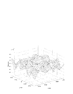
Fig. 5: Zoom of the refocused signals for the numerical experiment of Fig. 3 with processing $\Gamma=I$ (left), with a maximal amplitude of roughly $4\,10^{-3}$ and $\Gamma=\hbox{\rm Diag}(0,0,0,1)$ (right), with a maximal amplitude of roughly $0.035$.

The left figure shows no refocusing, in accordance with physical intuition and theory. The right figure shows that refocusing indeed occurs when only pressure in recorded (and its time derivative is set to $0$ in the solution of the wave equation presented in the appendix). Notice also that the refocused signal is roughly one half the one obtained in Fig. 4 as predicted by theory.

4.3 Refocusing of Other Classical Waves

The preceding sections deal with the refocusing of acoustic waves. The theory can however be extended to more complicated linear hyperbolic systems of the form (4) with $A({\bf x})$ a positive definite matrix, $D^{j}$ symmetric matrices, and ${\bf u}\in{\mathbb{C}}^{m}$. These include electromagnetic and elastic waves. Their explicit representation in the form (4) and expressions for the matrices $A({\bf x})$ and $D^{j}$ in these cases may be found in [24]. For instance, the Maxwell equations

$$\dfrac{\partial{{\bf E}}}{\partial{t}} = \frac{1}{\epsilon({\bf x})}\hbox{ curl }{\bf H}$$

$$\dfrac{\partial{{\bf H}}}{\partial{t}} = -\frac{1}{\mu({\bf x})}\hbox{curl }{\bf E}$$

may be written in the form (4) with ${\bf u}=({\bf E},{\bf H})\in{\mathbb{C}}^{6}$ and the matrix $A({\bf x})=\hbox{Diag}(\epsilon({\bf x}),\epsilon({\bf x}),\epsilon({\bf x}),\mu({\bf x}),\mu({\bf x}),\mu({\bf x}))$. Here $\epsilon({\bf x})$ is the dielectric constant (not to be confused with the small parameter $\varepsilon$), and $\mu({\bf x})$ is the magnetic permeability. The $6\times 6$ dispersion matrix $L({\bf x},{\bf k})$ for the Maxwell equations is given by

$$L({\bf x},{\bf k})=-\left(\begin{matrix}0&0&0&0&-k_{3}/\epsilon({\bf x})&k_{2}/\epsilon({\bf x})\cr 0&0&0&k_{3}/\epsilon({\bf x})&0&-k_{1}/\epsilon({\bf x})\cr 0&0&0&-k_{2}/\epsilon({\bf x})&k_{1}/\epsilon({\bf x})&0\cr 0&k_{3}/\mu({\bf x})&-k_{2}/\mu({\bf x})&0&0&0\cr-k_{3}/\mu({\bf x})&0&k_{1}/\mu({\bf x})&0&0&0\cr k_{2}/\mu({\bf x})&-k_{1}/\mu({\bf x})&0&0&0&0\cr\end{matrix}\right).$$

Generalization of our results for acoustic waves to such general systems is quite straightforward so we concentrate only on the modifications that need be made. The time reversal procedure is exactly the same as before: a signal propagates from a localized source, is recorded, processed as in (13) with a general matrix $\Gamma({\bf y}^{\prime})$, and re-emitted into the medium. The re-transmitted signal is given by (56). Furthermore, the equation for the adjoint Green’s matrix (57), the definition of the Wigner transform in section 3.4, and the expression (62) for the re-propagated signal still hold.

The analysis of the re-propagated signal is reduced to the study of the Wigner distribution, which is now modified. The mode decomposition need be generalized. We recall that

$$L({\bf x},{\bf k})=A_{0}^{-1}({\bf x})k_{j}D^{j}$$

is the $m\times m$ dispersion matrix associated with the hyperbolic system (4). Since $L({\bf x},{\bf k})$ is symmetric with respect to the inner product $\langle{\bf u},{\bf v}\rangle_{A_{0}}=(A_{0}{\bf u}\cdot{\bf v})$, its eigenvalues are real and its eigenvectors form a basis. We assume the existence of a time reversal matrix $\Gamma_{0}$ such that (21) holds with $\Gamma=\Gamma_{0}$ and such that $\Gamma_{0}^{2}=I$. For example, for electromagnetic waves $\Gamma_{0}=\hbox{Diag}(1,1,1,-1,-1,-1)$. Then the spectrum of $L$ is symmetric about zero and the eigenvalues $\pm\omega^{\alpha}$ have the same multiplicity. We assume in addition that $L$ is isotropic so that its eigenvalues have the form $\omega_{\pm}^{\alpha}({\bf x},{\bf k})=\pm c^{\alpha}({\bf x})|{\bf k}|$, where $c_{\alpha}({\bf x})$ is the speed of mode $\alpha$. We denote by $r_{\alpha}$ their respective multiplicities, assumed to be independent of ${\bf x}$ and ${\bf k}$ for ${\bf k}\not=0$. The matrix $L$ has a basis of eigenvectors ${\bf b}_{\pm}^{\alpha,j}({\bf x},{\bf k})$ such that

$$L({\bf x},{\bf k}){\bf b}_{\pm}^{\alpha,j}({\bf x},{\bf k})=\pm\omega^{\alpha}({\bf x},{\bf k}){\bf b}_{\pm}^{\alpha,j}({\bf x},{\bf k}),\quad j=1,\ldots,r_{\alpha},$$

and ${\bf b}_{\pm}^{\alpha,j}$ form an orthonormal set with respect to the inner product $\langle,\rangle_{A_{0}}$. The different $\omega_{\alpha}$ correspond to different types of waves (modes). Various indices $1\leq j\leq r_{\alpha}$ refer to different polarizations of a given mode. The eigenvectors ${\bf b}_{+}^{\alpha,j}$ and ${\bf b}_{-}^{\alpha,j}$ are related by

$$\Gamma_{0}{\bf b}_{+}^{\alpha,j}({\bf x},{\bf k})={\bf b}_{-}^{\alpha,j}({\bf x},{\bf k}),~{}~{}\Gamma_{0}{\bf b}_{-}^{\alpha,j}({\bf x},{\bf k})={\bf b}_{+}^{\alpha,j}({\bf x},{\bf k}).$$ (68)

Proposition 3 is then generalized as follows [14, 24]:

Proposition 4.

There exist scalar functions $a_{\pm}^{\alpha,jm}(t,{\bf x},{\bf k})$ such that

$$W(t,{\bf x},{\bf k})=\displaystyle\sum_{\pm,\alpha,j,m}a_{\pm}^{\alpha,jm}(t,{\bf x},{\bf k}){\bf b}_{\pm}^{\alpha,j}({\bf x},{\bf k})\otimes{\bf b}_{\pm}^{\alpha,m}({\bf x},{\bf k}).$$ (69)

Here the sum runs over all possible values of $\pm$, $\alpha$, and $1\leq j,m\leq r_{\alpha}$.

The main content of this proposition is again that the cross terms ${\bf b}_{\pm}^{\alpha,j}({\bf x},{\bf k})\otimes{\bf b}_{\mp}^{\beta,m}({\bf x},{\bf k})$ do not contribute, as well as the terms ${\bf b}_{\pm}^{\alpha,j}({\bf x},{\bf k})\otimes{\bf b}_{\pm}^{\alpha^{\prime},m}({\bf x},{\bf k})$ when $\alpha\not=\alpha^{\prime}$. This is because modes propagating with different speeds do not interfere constructively in the high frequency limit.

We may now insert expression (69) into (62) and obtain the following generalization of (63)

$$\hat{\bf u}^{B}({\bf k};{\bf x}_{0})=\displaystyle\sum_{\alpha,j,m}\left[a_{-}^{\alpha,mj}(T,{\bf x}_{0},{\bf k})\hat{S}_{+}^{\alpha,j}({\bf x}_{0},{\bf k}){\bf b}_{+}^{\alpha,m}({\bf x}_{0},{\bf k})\right.$$ (70)

$$~{}~{}~{}~{}~{}~{}~{}~{}~{}~{}~{}~{}~{}~{}~{}+\left.a_{+}^{\alpha,mj}(T,{\bf x}_{0},{\bf k})\hat{S}_{-}^{\alpha,j}({\bf x}_{0},{\bf k}){\bf b}_{-}^{\alpha,m}({\bf x}_{0},{\bf k})\right],$$

where $\hat{S}_{\pm}^{\alpha,j}({\bf k})=(A({\bf x}_{0})\hat{\bf S}({\bf k})\cdot{\bf b}_{\pm}^{\alpha,j}({\bf x}_{0},{\bf k})).$ This formula tells us that only the modes that are present in the initial source ($\hat{S}_{\pm}^{\alpha,j}({\bf k})\not=0$) will be present in the back-propagated signal but possibly with a different polarization, that is, $j\neq m$.

The initial conditions for the modes $a_{\pm}^{\alpha,jm}$ are given by

$$a_{\pm}^{\alpha,jm}(0,{\bf x},{\bf k})=|\chi({\bf x})|^{2}\hat{f}({\bf k})(A({\bf x})\Gamma({\bf x}){\bf b}_{\mp}^{\alpha,m}({\bf x},{\bf k})\cdot{\bf b}_{\pm}^{\alpha,j}({\bf x},{\bf k})),$$ (71)

which generalizes (64). When $\Gamma({\bf x})\equiv I$, we again obtain that $a_{\pm}^{\alpha,jm}(0,{\bf x},{\bf k})\equiv 0$, i.e., there is no refocusing as physically expected. When $\Gamma({\bf x})\equiv\Gamma_{0}$, we have for all $\alpha$ that

$$a_{\pm}^{\alpha,jm}(0,{\bf x},{\bf k})=|\chi({\bf x})|^{2}\hat{f}({\bf k})\delta_{jm}.$$

In a uniform medium the amplitudes $a_{\pm}^{\alpha,jm}$ satisfy an uncoupled system of free transport equations (45):

$$\dfrac{\partial{a_{\pm}^{\alpha,jm}}}{\partial{t}}\pm c_{\alpha}{\hat{\bf k}}\cdot\nabla_{\bf x}a_{\pm}^{\alpha,jm}=0,$$ (72)

which have no smoothing effect, and hence refocusing in a homogeneous medium is still poor. When $f({\bf x})=\delta({\bf x})$ and $\Omega=\mathbb{R}^{3}$, so that $\chi({\bf x})\equiv 1$, we still have that $a_{\pm}^{\alpha,jm}(T,{\bf x}_{0},{\bf k})=\delta_{jm}$ and refocusing is again perfect, that is, ${\bf u}^{B}(\boldsymbol{\xi};{\bf x}_{0})={\bf S}(\boldsymbol{\xi})$, as may be seen from (70).

4.4 The diffusive regime

The radiative transport regime holds when the matrices $A({\bf x})$ have the form

$$A({\bf x})=A_{0}({\bf x})+\sqrt{\varepsilon}A_{1}\Big{(}\dfrac{{\bf x}}{\varepsilon}\Big{)},$$

as in (47). Then the $r_{\alpha}\times r_{\alpha}$ coherence matrices $w_{\pm}^{\alpha}$ with entries $w_{\pm,jm}^{\alpha}=a_{\pm}^{\alpha,jm}$ satisfy a system of matrix-valued radiative transport equations (see [24] for the details) similar to (48). The matrix transport equations simplify considerably in the diffusive regime, such as the one considered in section 3.8 when waves propagate over large distances and long times. We assume for simplicity that $A_{0}=A_{0}({\bf x})$ and $\Gamma=\Gamma({\bf x})$ are independent of ${\bf x}$. Polarization is lost in this regime, that is, $a^{\alpha,jm}(t,{\bf x},{\bf k})=0$ for $j\not=m$ and wave energy is equidistributed over all directions. This implies that

$$a_{+}^{\alpha,jj}(t,{\bf x},{\bf k})=a_{-}^{\alpha,jj}(t,{\bf x},{\bf k})=a_{\alpha}(t,{\bf x},|{\bf k}|)$$

so that $a^{\alpha,jj}$ is independent of $j=1,\dots,r_{\alpha}$ and of the direction ${\hat{\bf k}}={\bf k}/|{\bf k}|$. Furthermore, because of multiple scattering, a universal equipartition regime takes place so that

$$a_{\alpha}(t,{\bf x}_{0},|{\bf k}|)=\phi(t,{\bf x}_{0},c_{\alpha}|{\bf k}|),$$ (73)

where $\phi(t,{\bf x},\omega)$ solves a diffusion equation in ${\bf x}$ like (51) (see [24]). The diffusion coefficient $D(\omega)$ may be expressed explicitly in terms of the power spectra of the medium fluctuations [24]. Using (71) and (73), we obtain when $f$ is isotropic the following initial data for the function $\phi$

$$\phi(0,{\bf x},\omega)=\dfrac{1}{4\pi}|\chi({\bf x})|^{2}\displaystyle\int_{S^{2}}\dfrac{2}{|\alpha|}\displaystyle\sum_{j,\omega_{\alpha}>0}\hat{f}\Big{(}\dfrac{\omega}{c_{\alpha}}\Big{)}(A_{0}\Gamma{\bf b}_{-}^{\alpha,j}(\hat{\bf k}),{\bf b}_{+}^{\alpha,j}(\hat{\bf k}))d\Omega(\hat{\bf k}),$$ (74)

where $|\alpha|$ is the number of non-vanishing eigenvalues of $L({\bf x},{\bf k})$, and $d\Omega(\hat{\bf k})$ is the Lebesgue measure on the unit sphere $S^{2}$.

Let us assume that non-propagating modes are absent in the initial source ${\bf S}({\bf x})$, that is, $\hat{S}_{0}^{j}({\bf k})=0$ with the subscript zero referring to modes corresponding to $\omega_{0}=0$. Then (70) becomes

$$\hat{\bf u}({\bf k};{\bf x}_{0})=\displaystyle\sum_{\alpha,j}\phi(T,{\bf x}_{0},c_{\alpha}|{\bf k}|)\left[\hat{S}_{+}^{\alpha,j}({\bf k}){\bf b}_{+}^{\alpha,j}({\bf x}_{0},{\bf k})+\hat{S}_{-}^{\alpha,j}({\bf k}){\bf b}_{-}^{\alpha,j}({\bf x}_{0},{\bf k})\right].$$ (75)

This is an explicit expression for the re-propagated signal in the diffusive regime, where $\phi$ solves the diffusion equation (51) with initial conditions (74).

5 Conclusions

This paper presents a theory that quantitatively describes the refocusing phenomena in time reversal acoustics as well as for more general processings of other classical waves. We show that the back-propagated signal may be expressed as the convolution (1) of the original source ${\bf S}$ with a filter $F$. The quality of the refocusing is therefore determined by the spatial decay of the kernel $F$. For acoustic waves, the explicit expression (39) relates $F$ to the Wigner distribution of certain solutions of the wave equation. The decay of $F$ is related to the smoothness in the phase space of the amplitudes $a_{j}(t,{\bf x},{\bf k})$ defined in Proposition 3. The latter satisfy a free transport equation in homogeneous media, which sharpens the gradients of $a_{j}$ and leads to poor refocusing. In contrast, the amplitudes $a_{j}$ satisfy the radiative transport equation (48) in heterogeneous media, which has a smoothing effect. This leads to a rapid spatial decay of the filter $F$ and a better refocusing. For longer times, $a_{j}$ satisfies a diffusion equation. This allows for an explicit expression (54)-(55) of the time reversed signal. The same theory holds for more general waves and more general processing procedures at the recording array, which allows us to describe the refocusing of electromagnetic waves when only one component of the electric field is measured, for instance.

Appendix

This appendix presents the details of the numerical simulation of (10). We assume that $\rho$ is constant and that only $\kappa({\bf x})$ fluctuates. We can therefore recast (10) as

$$\dfrac{\partial^{2}{p}}{\partial{t}^{2}}-c^{2}({\bf x})\Delta p=0.$$

The above wave equation is discretized using a second-order scheme (three point stencil in every variable) both in time and space. The resolution in time is explicit and time reversible, i.e., the equation that yields $p(t_{n+1})$ from $p(t_{n-1})$ and $p(t_{n})$ can be used to retrieve $p(t_{n-1})$ exactly from $p(t_{n})$ and $p(t_{n+1})$. We write $c^{2}({\bf x})=c_{0}^{2}+c_{1}^{2}({\bf x})$. The average velocity is $c_{0}^{2}=1$. The random part $c_{1}^{2}$ has been constructed as follows. Let $2N\times 2N$ be the number of spatial grid points and $c_{1;n,m}^{2}$ be the value of $c_{1}^{2}$ at the grid point $(n,m)$. The values $c^{2}_{1;2n,2m}$ have been chosen independently and uniformly on $(-r,r)$ with $r<1/2$. The value of $c_{1}^{2}$ is then set constant on four adjacent pixels by enforcing that $c^{2}_{1;2n-1,2m}=c^{2}_{1;2n-1,2m-1}=c^{2}_{1;2n,2m-1}=c^{2}_{1;2n,2m}$ for $1\leq n,m\leq N$. In all simulations, we have $N=200$, which generates a grid of $400^{2}=1.6\,10^{4}$ points. The time step has been chosen so that the CFL condition $\delta t<\min\limits_{{\bf x}}c({\bf x})/(2N)$ is ensured.

References

- [1] G. Bal and L. Ryzhik, Time Reversal for Classical Waves in Random Media, C. R. Acad. Sci. Paris, Série I, 333 (2001), pp. 1041–1046.
- [2] C. Bardos and M. Fink, Mathematical foundations of the time reversal mirror, Preprint, (2001).
- [3] J. Berryman, L. Borcea, G. Papanicolaou, and C. Tsogka, Imaging and time reversal in random media, Submitted to JASA, (2001).
- [4] P. Blomgren, G. Papanicolaou, and H. Zhao, Super-Resolution in Time-Reversal Acoustics, to appear in J. Acoust. Soc. Am., (2001).
- [5] J. F. Clouet and J. P. Fouque, A time-reversal method for an acoustical pulse propagating in randomly layered media, Wave Motion, 25 (1997), pp. 361–368.
- [6] R. Dautray and J.-L. Lions, Mathematical Analysis and Numerical Methods for Science and Technology. Vol.6, Springer Verlag, Berlin, 1993.
- [7] A. Derode, P. Roux, and M. Fink, Robust Acoustic Time-Reversal With High-Order Multiple-Scattering, Phys. Rev. Lett., 75 (1995), pp. 4206–9.
- [8] D. R. Dowling and D. R. Jackson, Narrow-band performance of phase-conjugate arrays in dynamic random media, J. Acoust. Soc. Am., 91(6) (1992), pp. 3257–3277.
- [9] L. Erdös and H. T. Yau, Linear Boltzmann equation as the weak coupling limit of a random Schrödinger Equation, Comm. Pure Appl. Math., 53(6) (2000), pp. 667–735.
- [10] N. Ewodo, Refocusing of a time-reversed acoustic pulse propagating in randomly layered media, Jour. Stat. Phys., 104 (2001), pp. 1253–1272.
- [11] M. Fink, Time reversed acoustics, Physics Today, 50(3) (1997), pp. 34–40.
- [12] , Chaos and time-reversed acoustics, Physica Scripta, 90 (2001), pp. 268–277.
- [13] M. Fink and C. Prada, Acoustic time-reversal mirrors, Inverse Problems, 17(1) (2001), pp. R1–R38.
- [14] P. Gérard, P. A. Markowich, N. J. Mauser, and F. Poupaud, Homogenization limits and Wigner transforms, Comm. Pure Appl. Math., 50 (1997), pp. 323–380.
- [15] F. Golse, P.-L. Lions, B. Perthame, and R. Sentis, Regularity of the moments of the solution of a transport equation, Journal of Functional Analysis 76, (1988), pp. 110–125.
- [16] W. Hodgkiss, H. Song, W. Kuperman, T. Akal, C. Ferla, and D. Jackson, A long-range and variable focus phase-conjugation experiment in a shallow water, J. Acoust. Soc. Am., 105 (1999), pp. 1597–1604.
- [17] A. Ishimaru, Wave Propagation and Scattering in Random Media, New York: Academics, 1978.
- [18] S. R. Khosla and D. R. Dowling, Time-reversing array retrofocusing in noisy environments, J. Acous. Soc. Am., 109(2) (2001), pp. 538–546.
- [19] W. Kuperman, W. Hodgkiss, H. Song, T. Akal, C. Ferla, and D. Jackson, Phase-conjugation in the ocean, J. Acoust. Soc. Am., 102 (1997), pp. 1–16.
- [20] E. W. Larsen and J. B. Keller, Asymptotic solution of neutron transport problems for small mean free paths, J. Math. Phys., 15 (1974), pp. 75–81.
- [21] P.-L. Lions and T. Paul, Sur les mesures de Wigner, Rev. Mat. Iberoamericana, 9 (1993), pp. 553–618.
- [22] M. Mokhtar-Kharroubi, Mathematical Topics in Neutron Transport Theory, World Scientific, Singapore, 1997.
- [23] G. Papanicolaou, L. Ryzhik, and K. Solna, The parabolic approximation and time reversal in a random medium, preprint, (2001).
- [24] L. Ryzhik, G. Papanicolaou, and J. B. Keller, Transport equations for elastic and other waves in random media, Wave Motion, 24 (1996), pp. 327–370.
- [25] P. Sheng, Introduction to Wave Scattering, Localization and Mesoscopic Phenomena, Academic Press, New York, 1995.
- [26] H. Spohn, Derivation of the transport equation for electrons moving through random impurities, Jour. Stat. Phys., 17 (1977), pp. 385–412.