Modeling of Spiking-Bursting Neural Behavior Using Two-Dimensional Map

Abstract

A simple model that replicates the dynamics of spiking and spiking-bursting activity of real biological neurons is proposed. The model is a two-dimensional map which contains one fast and one slow variable. The mechanisms behind generation of spikes, bursts of spikes, and restructuring of the map behavior are explained using phase portrait analysis. The dynamics of two coupled maps which model the behavior of two electrically coupled neurons is discussed. Synchronization regimes for spiking and bursting activity of these maps are studied as a function of coupling strength. It is demonstrated that the results of this model are in agreement with the synchronization of chaotic spiking-bursting behavior experimentally found in real biological neurons.

]

I Introduction

Understanding dynamical principles and mechanisms behind the control of activity, signal and information processing that occur in neurobiological networks is hardly possible without numerical studies of collective dynamics of large networks of neurons. These simulations need to take into account the complex architecture of couplings among individual neurons that is suggested by data from biological experiments. One of the complicating factors in understanding the simulation results is the complexity of temporal behavior of individual biological neurons. This complexity is due to the large number of ionic currents involved in the nonlinear dynamics of neurons. As a result, realistic channel-based models proposed for a single neuron is usually a system of many nonlinear differential equations (see, for example [1, 2, 3, 4, 5] and the review of the models in [6]). The strong nonlinearity and high dimensionality of the phase space is a significant obstacle in understanding the collective behavior of such dynamical systems. The dynamical mechanisms responsible for restructuring collective behavior of a network of channel-based neuron models are difficult or impossible to analyze because these mechanisms are well hidden behind the complexity of the equations. If there is a chance to identify possible dynamical mechanisms behind a particular behavior of the network without the use of complex models, then this knowledge can be used to guide through numerical study of this behavior with the high-dimensional channel-based models. Based on these results one can specify the actual dynamical mechanism occurred in the network and understand the biological processes which contribute to it.

One way to reveal the dynamical mechanisms is to use a simplified or phenomenological model of the neuron. However, many experiments indicate the restructuring of collective behavior utilizes a variety of dynamical regimes generated by individual dynamics of a neuron. When neural dynamics include the regime chaotic spiking-bursting oscillations the system of differential equations describing each neuron should be at least a three-dimensional system (see for example [7]). Further simplification of phenomenological models for complex dynamics of the neuron can be obtain using dynamical systems in the form of a map. Despite the low-dimensional phase space of this nonlinear map, it is able to demonstrate a large variety of complex dynamical regimes.

The use of low-dimensional model maps can be useful for understanding the dynamical mechanisms if they mimic the dynamics of oscillations observed in real neurons, show correct restructuring of collective behavior, and are simple enough to study the reasons behind such restructuring. The development of a model map which is capable of describing various types of neural activity, including generation of tonic spikes, irregular spiking, and both regular and irregular bursts of spikes, is the goal of this paper.

It is known that constructing a low-dimensional system of differential equation which is capable of generating fast spikes bursts excited on top of the slow oscillations, one needs to consider a system which has both slow and fast dynamics (see for example [7, 8, 9, 10, 11]). Using the same approach one can construct a two-dimensional map, which can be written in the form

$$x_{n+1} = f(x_{n},y_{n}+\beta_{n})~{},$$ (1a)

$$y_{n+1} = y_{n}-\mu(x_{n}+1)+\mu\sigma_{n}~{},$$ (1b)

where $x_{n}$ is the fast and $y_{n}$ is the slow dynamical variable. Slow time evolution of $y_{n}$ is due to small values of the parameter $\mu=0.001$. Terms $\beta_{n}$ and $\sigma_{n}$ describe external influences applied to the map. These terms model the dynamics of the neuron under the action of the external DC bias current $I_{DC}$ and synaptic inputs $I^{syn}_{n}$. The term $\sigma_{n}$ can also be used as the control parameter to select the regime of individual behavior.

A model in the form of two-dimensional map, whose form is similar to (1) was used in the study of dynamical mechanisms behind the emergence and regularization of chaotic bursts in a group of synchronously bursting cells coupled through a mean field[12, 13]. The effect of anti-phase regularization was also modeled before with one-dimensional maps [14]. In both these models the oscillations during the burst were described by a chaotic trajectory. Map (1) improves these models by adding a feature that enables one to mimic the dynamics of individual spikes within the burst. This is achieved using a modification of the shape of the nonlinear function $f(x,y)$ which is now a discontinuous function of the form

$$f(x,y)=\cases{\alpha/(1-x)+y,&$x\leq 0$\cr\alpha+y,&$0<x<\alpha+y$\cr-1,&$x\geq\alpha+y$\cr}$$ (2)

where $\alpha$ is a control parameter of the map. The dependence of $f(x,y)$ on $x$ computed for a fixed value of $y$ is shown in Fig.1. In this plot the values of $\alpha$ and $y$ are set to illustrate the possibility of coexistence of limit cycle, $P_{k}$, corresponding to spiking oscillation in (1a), and fixed points $x_{ps}$ and $x_{pu}$. Note that when $y$ increases or decreases the graph of $f(x,y)$ moves up or down, respectively, except for the third interval $x\geq\alpha+y$, where the values of $f(x,y)$ always remain equal to -1.

FIG. 1.: The shape of the nonlinear function $f(x,y)$, plotted for $\alpha=6.0$ and $y=-3.93$, is shown with a solid line. The dashed line illustrates a super-stable cycle $P_{k}$ of the fast map (3a), where the value of $y$ is fixed. The stable and unstable fixed points of the map are indicated by $x_{ps}$ and $x_{pu}$, respectively.

The paper is organized as follows: Section II considers the features of the fast and slow dynamics which explain the formation of various types of behavior in the isolated map. It also discusses the bifurcations responsible for the qualitative change of activity. The dynamics of response generated by the map after it is excited or inhibited by an external pulse is discussed in Section III. The goal of this section is to illustrate dynamical mechanisms that control the response, and to show how the relation between the two inputs of the map influence the properties of the response. Section IV presents the results of a synchronization study in two coupled maps.

II Individual Dynamics of the Map

Consider the regimes of oscillations produced by the individual dynamics of the map. In this case the inputs $\beta_{n}=\beta$ and $\sigma_{n}=\sigma$ are constants. Note that if $\beta$ is a constant, then it can be omitted from the equations using the change of variable $y_{n}+\beta\rightarrow y_{n}^{new}$. Therefore, the individual dynamics of the map depends only on the control parameters $\alpha$ and $\sigma$, and the map can be rewritten in the form

$$x_{n+1} = f(x_{n},y_{n}),$$ (3a)

$$y_{n+1} = y_{n}-\mu(x_{n}+1)+\mu\sigma~{}.$$ (3b)

Typical regimes of temporal behavior of the map are shown in Figs 2 and 3. When the value of $\alpha$ is less then 4.0 then, depending on the value of parameter $\sigma$, the map generates spikes or stays in a steady state (see Fig 2). The frequency of the spikes increases as the value of parameter $\sigma$ is increased (see Fig 2).

FIG. 2.: Waveforms of spiking behavior generated by map (3) with $\alpha=4$. Panel (a) shows the transition to the regime of silence for $\sigma=-0.01$. The regimes of continuous tonic spiking are computed for $\sigma=0.01$ (b) and $\sigma=0.1$ (c).

For $\alpha>4$ the map dynamics are capable of producing bursts of spikes. The spiking-bursting regimes are found in the intermediate region of parameter $\sigma$ between the regimes of continuous tonic spiking and steady state (silence). The spiking-bursting regimes include both periodic and chaotic bursting. A few typical bursting-spiking regimes computed for different values of $\sigma$ are presented in Fig 3.

Due to the two different time scales involved in the dynamics of the model, the mechanisms behind the restructuring of the dynamical behavior can be understood through the analysis of the fast and slow dynamics separately. In this case, time evolution of the fast variable, $x$, is studied with the one-dimensional map (3a) where the slow variable, $y$, is treated as a control parameter whose value drifts slowly in accordance with equation (3b). It follows from (3b) that the value of $y$ remains unchanged only if $x=x_{s}$ given by

$$x_{s}=-1+\sigma.$$ (4)

If $x<x_{s}$, then the value of $y$ slowly increases. If $x>x_{s}$, then $y$ decreases.

FIG. 3.: Typical waveforms of the spiking-bursting behavior generated by the map (3) for the following parameter values: $\alpha=4.5$, $\sigma=0.14$ (a); $\alpha=6.0$, $\sigma=-0.1$ (b); and $\alpha=6.0$, $\sigma=0.386$ (c).

From (3a) one can find the equation for the coordinate of fixed points $x_{p}$ of the fast map. This equation is of form

$$y=x_{p}-\frac{\alpha}{1-x_{p}},$$ (5)

where $x_{p}\leq 0$. Equation (5) defines the branches of slow motion in the two-dimensional phase space $(x_{n},y_{n})$ (see Fig 4). The stable branch $S_{ps}(y)$ exists for $x_{p}<1-\sqrt{\alpha}$ and the unstable branch $S_{pu}(y)$ exists within $1-\sqrt{\alpha}\leq x_{p}\leq 0$

Considering the fast and slow dynamics together, one can see that, if $x_{s}$ is in the stable branch $S_{ps}(y)$, then the map (3) has a stable fixed point. The stable fixed point corresponds to the regime of silence in the neural dynamics. The oscillations in the map dynamics will appear when $x_{s}>1-\sqrt{\alpha}$. This is the threshold of excitation, which corresponds to the bifurcation values of $\sigma$ given by

$$\sigma_{th}=2-\sqrt{\alpha}.$$ (6)

To understand the dynamics of excited neurons within this model one needs to consider branches that correspond to the spiking regime. To evaluate the location of the spiking branches, consider the mean value of $x_{n}$ computed for the periodic trajectory of the fast map (3a) as a function of $y$. Here $y$ is treated as a parameter. Use of such an approximation is quite typical for an analysis involving fast and slow dynamics. It works well for small values of parameter $\mu$.

It follows from the shape of $f(x,y)$ that for any value of $y$, map (3a) generates no more than one periodic trajectory $P_{k}$, where $k$ is the period (i.e. $x_{n}=x_{n+k}$). The cycles $P_{k}$ always contain the point $x_{n}=-1$ and the index $k$ increases stepwise ($k\rightarrow k+1$) as $y$ decreases. Since the trajectory $P_{k}$ always has a point in the flat interval of $f(x,y)$, all these cycles are super-stable except for bifurcation values of $y$ for which the trajectory contains the point $x_{n}=0$ (see Fig 1). The location of the spiking branch, $S_{spikes}$, of ”slow” motion in the phase plane ($x_{n},y_{n}$) can be estimated as the mean value of $x$ computed for the period of cycle $P_{k}$,

$$x_{mean}=\frac{1}{k}\sum_{m=1}^{k}f^{(m)}(-1,y),$$ (7)

where $k$ is the period of $P_{k}$, and $f^{(m)}(x,y)$ is the $m$-th iterate of (3a), started at point $x$ and computed for fixed $y$. The spiking branch of ”slow” dynamics evaluated with (7) is shown in Fig4. One can see that this branch has many discontinuities caused by the bifurcations of the super-stable cycles $P_{k}$.

To complete the picture of fast and slow dynamics of the model for $\alpha>4$, one needs to consider the fast map bifurcation associated with the formation of homoclinic orbit $h_{pu}$ originating from the unstable fixed point, $x_{pu}$. This homoclinic orbit occurs when the coordinate of $x_{pu}$ become equal to -1. It can be easily shown that such a situation can take place only if $\alpha>4$. The homoclinic orbit forms at the value of $y$ where the unstable branch $S_{pu}(y)$ crosses the line $x=-1$, see Fig.4b. When the map is firing spikes and the value of $y$ gets to the bifurcation point, the cycle $P_{k}$ merges into the homoclinic orbit, disappears, and then the trajectory of the map jumps to the stable fixed point $x_{ps}$.

Typical phase portraits of the model, obtained under the assumptions made above, are presented in Fig.4. Fig.4a shows the typical behavior for $2<\alpha\leq 4$. Here, only two regimes are generated. The first regime is the state of silence, when the operating point (OP), given by the intersection of $x_{s}=-1+\sigma$ and one of the branches, is on the branch $S_{ps}(y)$. The second regime is the regime of tonic spiking, when the operating point is selected on the spiking branch $S_{spikes}$.

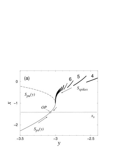
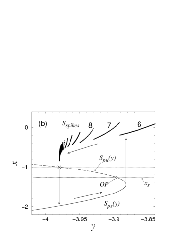
FIG. 4.: Stable ($S_{ps}(y)$, $S_{spikes}$) and unstable ($S_{pu}(y)$) branches of slow dynamics of (3) plotted on the plane of phase variables ($y,x$). The cases of $\alpha=4$ and $\alpha=6$ are presented in (a) and (b), respectively. Numbers on the branch $S_{spikes}$ stand for the value of $k$ of the cycles $P_{k}$. The operating points $OP$ are selected to illustrate the regime of silence in (a) and the regime of spiking-bursting oscillations in (b). Arrows indicate the direction of slow evolution along the branches, and switching in the case of (b).

When $\alpha>4$ the picture changes qualitatively (see Fig 4b). Now, stable branches $S_{ps}(y)$ and $S_{spikes}$ are separated by the unstable branch $S_{pu}(y)$. If the operating point is selected on $S_{pu}(y)$, then the phase of silence, corresponding to slow motion along $S_{ps}(y)$, and spiking, when system moves along $S_{spikes}$, alternate forming the regime of spiking-bursting oscillations. The beginning of a burst of spikes corresponds to the bifurcation state of the fast map where fixed points $x_{ps}$ and $x_{pu}$ merge together and disappear. Before this bifurcation the system is in $x_{ps}$ and, therefore, $y$ increases. The termination of the burst is due to the bifurcation of the fast map associated with the formation of the homoclinic orbit $h_{pu}$. Here, the limit cycle of the spiking mode merges into the homoclinic orbit and disappears. After that the fast subsystem flips to the stable fixed point $x_{ps}$. Then the process repeats (see arrows in Fig 4b).

It is clear from Fig.4a that when operating point is set on $S_{ps}(y)$ the model will be in the regime of silence. When the operating point is set on the branch $S_{spikes}$ the model produces tonic spiking, unless the point is set close to the formation of homoclinic orbit $h_{pu}$. One can see that, at the vicinity of this bifurcation, the branch $S_{spikes}$ becomes densely folded. As a result, the behavior of $y$, which is governed by the mean value of $x_{n}$, can become extremely sensitive to small perturbations and even lead to instability caused by high-gain feedback. This is one of the reasons for the irregular, chaotic spiking-bursting behavior which occurs in the map when the operating point is set close to the area of the branch $S_{spikes}$ where this branch is densely folded. The detailed and rigorous analysis of chaotic dynamics cannot be done within the approximations made above and require more precise computation of $S_{spikes}$ which is beyond the scope of this paper.

FIG. 5.: Bifurcation diagram on the parameter plane ($\sigma,\alpha$).

The results of the analysis presented above are summarized in the sketch of the bifurcation diagram plotted on the parameter plain ($\sigma,\alpha$) (see Fig 5). The bifurcation curve $\sigma_{th}$ corresponds to the excitation threshold (6) where the fixed point of the 2-d map becomes unstable and the map starts generating spikes. Curve $L_{ts}$ shows the approximate location of the border between spiking and spiking-bursting regimes, obtained in the numerical simulations. Note that separation of spiking and bursting regimes is not always obvious, especially in the regime of chaotic spiking. The regime of spiking-bursting oscillations takes place within the upper triangle formed by curves $\sigma_{th}$ and $L_{ts}$. The regimes of chaotic spiking or spiking-bursting behavior are found in the relatively narrow region of the parameters located around $L_{ts}$. This region contains complex structure of bifurcations, associated with multi-stable regimes, and is not shown in Fig 5.

The bifurcation diagram shows the role of control parameters in the selection of dynamical features of the considered neuron model. Both parameters can be used to mimic a particular type of neural behavior. Parameter $\sigma$ can be used to model the external DC current injection that depolarizes or hyperpolarizes the neuron. In this case $\sigma$ can be written as

$$\sigma=\sigma_{u}+I_{DC},$$ (8)

where $\sigma_{u}$ is the parameter that selects the dynamics of isolated neuron, and $I_{DC}$ is the parameter that models the DC current injected into the cell. The changes in behavior caused by $I_{DC}$ are similar to the action of the parameter $I$ in the well known Hindmarsh-Rose model [7].

If the individual dynamics of the modelled neuron are capable of generating only regimes of silence and tonic spiking, and do not support the regime of bursts of spikes, then the value of $\alpha$ should be set below 4. In this case, no matter what the level of $I_{DC}$ injected is, the system will not show bursts of spikes (see Fig 5).

III Modeling of Response to the Injection of Current

To study the dynamical regimes of neuronal behavior in experiments, biologists change the type of neural activity using the injection of electrical current into the cell though an electrode. It was shown above that the injection of DC current can be modeled in the map (1) using parameter $\sigma_{n}=\sigma$ (see equation (8)). In this case, since the external influence does not vary in time, the role of parameter $\beta_{n}=\beta$ is not important, because the behavior of the map after the transient is independent of the value of $\beta$. However, when the injected current changes in time, it may be useful to consider the dynamics of parameter $\beta_{n}$ in order to provide more realistic modeled behavior during the transient. Taking this into account, the input of the model can be considered in the form:

$$\beta_{n}=\beta^{e}I_{n}~{},~{}~{}\sigma_{n}=\sigma^{e}I_{n},$$ (9)

where $I_{n}$ is injected current, and coefficients $\beta^{e}$ and $\sigma^{e}$ are selected to achieve the desired properties of response behavior.

This Section briefly illustrates how the relation between these coefficients effects the dynamics of response to the pulse of $I_{n}$. To be specific, consider the map in the regime of tonic spiking with $\alpha=5.0$, $\sigma=0.33$, $\beta=0$. To study the response behavior, positive and negative pulses of amplitude 0.8 and duration of 100 iterations were applied to the continuously spiking map. In the simulations presented below the coefficient $\sigma^{e}$ was selected to be equal to one.

FIG. 6.: Response of the model with $\sigma^{e}=1$ and $\beta^{e}=0$ to a positive pulse of $I_{n}$. The parameters of the map are selected in the regime of tonic spiking ($\alpha=5.0$, $\sigma=0.33$, $\beta=0$).

FIG. 7.: Response of the model with $\sigma^{e}=1.0$ and $\beta^{e}=0$ to a negative pulse of $I_{n}$. The parameters of the map are selected in the regime of tonic spiking ($\alpha=5.0$, $\sigma=0.33$, $\beta=0$).

Figures 6 and 7 show the response to the positive and negative pulse, respectively, computed with $\beta^{e}=0$. In this case, during the action of a positive pulse, the value of $y_{n}$ increases monotonically because of the increased value of $\sigma_{n}$ (see (1b)). The increase of $y_{n}$ pushes the fast map up, see Fig 1. This leads to an increase in the frequency of spiking. After the action of the pulse ends the value of $y_{n}$ monotonically decreases back to the original state (see Fig. 6).

When a negative pulse is applied, it pushes the operating point down and, if the amplitude of the pulse is sufficiently large, shuts off the regime of spiking (see Fig.7). This happens because the trajectory of the fast map gets to the perturbed operating point which is now on the stable branch $S_{ps}(y)$, (see Fig 4b). After the pulse is over the spiking does not re-appear immediately because the system spends some time drifting along the stable branch of slow motions $S_{ps}(y)$, during which the variable $y$ overshoots its original value for the spiking regime. As a result, after the system switches to the spiking branch $S_{spikes}$, $y_{n}$ monotonically drifts down to the unperturbed operating point. The dynamics of the slow evolution are clearly seen in the lower panel of Fig.7.

FIG. 8.: Response of the model with $\sigma^{e}=1.0$ and $\beta^{e}=1.0$ to a positive pulse of $I_{n}$. The parameters of the map are selected in the regime of tonic spiking ($\alpha=5.0$, $\sigma=0.33$, $\beta=0$).

FIG. 9.: Response of the model with $\sigma^{e}=1.0$ and $\beta^{e}=1.0$ to a negative pulse of $I_{n}$. The parameters of the map are selected in the regime of tonic spiking ($\alpha=5.0$, $\sigma=0.33$, $\beta=0$).

Figures 8 and 9 illustrate how response to the pulse of $I_{n}$ changes when coefficient $\beta_{n}$ is not equal to zero. To be brief and specific consider the case of $\beta^{e}=1.0$ and $\sigma^{e}=1.0$. Comparing Fig.8 with Fig.6 one can see that the response dynamics to the positive pulse changes qualitatively. Indeed, when the pulse current is applied, then, acting through $\beta_{n}$, it immediately forces the fast map to shift up. As a result, the rate of spiking and mean value of $x_{n}$ increases sharply. Variable $y_{n}$ reacts to this change and decreases its value to compensate for the sudden change of the mean value of $x_{n}$. When the action of the pulse is over, the value of $\beta_{n}$ returns to its original value and, due to the updated levels of $y_{n}$, the fast map overshoots its original state. As a result, the trajectory of the fast map reaches the stable fixed point. To return to the original regime of spiking the system has to go all the way along the branches of slow motion $S_{ps}(y)$ and $S_{spikes}$ back to the original operating point (see Fig. 4b). This type of response is observed in real neurobiological experiments, see for example [15].

Using the same analysis one can understand the new effects in the response to a negative pulse caused by the action of $\beta_{n}$. These new effects can be clearly seen comparing Fig.9 with Fig. 7.

The presented results illustrate how 2-d map (1) along with equation (9) can model a large variety of transient neural behavior induced by injected current. Due to the simplicity of the model one can clearly see the nonlinear mechanisms behind the response behavior and apply them to select the desired balance between $\sigma^{e}$ and $\beta^{e}$ to model a particular type of response.

IV Regimes of synchronization in two coupled maps

This section presents the results of studies of synchronization regimes in coupled chaotically bursting 2-d maps. The goal of this study is to reproduce the main regimes of synchronous behavior found in a real neurobiological experiment [16]. The experiment was carried out on two electrically coupled neurons (the pyloric dilators, PD) from the pyloric CPG of the lobster stomatogastric ganglion [17]. The regimes found in the experiment were also reproduced in numerical simulations using Hindmarsh-Rose model [18, 19], one-dimensional map model [14], and in experiments with electronic neurons [19].

The equations used in the numerical simulations of the coupled maps are of form

$$x_{i,n+1} = f(x_{i,n},y_{i,n}+\beta_{i,n}),$$ (10)

$$y_{i,n+1} = y_{i,n}-\mu(x_{i,n}+1)+\mu\sigma_{i}+\mu\sigma_{i,n},$$ (11)

where index $i$ specifies the cell, and $\sigma_{i}$ is the parameter that defines the dynamics of the uncoupled cell. The coupling between the cells is provided by the current flowing from one cell to the other. This coupling is modeled by

$$\beta_{i,n} = g_{ji}\beta^{e}(x_{j,n}-x_{i,n})$$ (12)

$$\sigma_{i,n} = g_{ji}\sigma^{e}(x_{j,n}-x_{i,n})$$ (13)

where $i\neq j$, and $g_{ji}$ is the parameter characterizing the strength of the coupling. The coefficients $\beta^{e}$, $\sigma^{e}$ set the balance between the couplings for the fast and slow processes in the cells, respectively. In the numerical simulations the values of the coefficients are set to be equal: $\beta^{e}=1.0$ and $\sigma^{e}=1.0$. The other parameters of the coupled maps (11) that remain unchanged in the simulations have the following values: $\mu=0.001$, $\alpha_{1}=4.9$, $\alpha_{2}=5.0$. The coupling between the maps is symmetrical, $g_{ji}=g_{ij}=g$.

FIG. 10.: Waveforms generated by the two coupled 2-d maps (11) with $\sigma_{1}=0.240$ and $\sigma_{2}=0.245$. Waveforms of $x_{1,n}$ and $x_{2,n}$ are shown by solid and dashed lines, respectively. Three different regimes of spiking-bursting behavior are shown. Individual chaotic spiking-bursting oscillations of uncoupled maps, $g=0.0$, - (a). Regime of synchronized chaotic bursts, computed with $g=0.043$, - (b). Regime of antiphase synchronization, computed with $g=-0.029$, -(c).

First, consider the main regimes of synchronization between the maps generating irregular, chaotic bursts of spikes. To set the individual dynamics of the maps to this regime, the parameters $\sigma_{i}$, that take into account the DC bias current injected into the neurons (see [16] for details), are tuned to the following values: $\sigma_{1}=0.240$, $\sigma_{2}=0.245$. When these maps are uncoupled ($g=0$) they produce chaotic spiking-bursting oscillations shown in Fig 10a. When the coupling becomes sufficiently large the slow components of the bursts synchronize while spikes within the bursts remain asynchronous see the waveforms in Fig. 10b obtained with $g=0.043$. This regime of synchronization is typical for naturally coupled PD neurons (see Figure 2a in [16]).

Introduction of negative coupling, $g<0$, also leads to synchronization of bursts, but in this regime of synchronization the systems burst in antiphase. Typical waveforms produced in this regime are presented in Fig. 10c. This regime of synchronization of chaotic bursts is also observed in the experimental study of coupled PD neurons (see Figure 2c in  [16]). It is important to emphasize that, both in this simulation and in the experiment, the regime of antiphase synchronization characterized by the onset of regular bursts.

The simplicity of this model enables one to understand the possible cause for the onset of regular bursting in the antiphase synchronization. It is shown in Section II that chaotic dynamics of bursts occurs when the operating point of the system appears close to the leftmost area of the spiking branch $S_{spikes}$. In this region, $S_{spikes}$ is densely folded and, if system slows down in this area, the timing for the end of the burst becomes very sensitive to infinitesimal perturbations.

FIG. 11.: Attractors computed from the waveforms of the first cell operating in the regime of uncoupled oscillations - (a) and in the regime of antiphase synchronization - (b). Waveforms for these regimes are shown in Fig. 10a and Fig. 10c, respectively. The points of the attractors are connected by lines to clearly show their sequence in time.

This fact is illustrated in Fig. 11a. This figure shows the attractor computed from the waveforms $x_{1,n}$ and $y_{1,n}$ of the first cell when the cells are uncoupled (this regime is shown in Fig. 10a). To plot the attractor, the waveforms of $x_{1,n}$ and $y_{1,n}$ were filtered by a fourth order low-pass filter with cutoff frequency 0.6. As a result, the attractor does not contain sharp spikes and the approximate location $S_{spikes}$, which is close to the center of filtered spiking oscillations, is easy to see. The level of coordinate $x_{f}$, corresponding to the operating point, is equal to $x_{s}=-1+\sigma_{1}=-0.76$. One can see from Fig. 11a that when the center of oscillations gets close to that level the trajectory becomes rather complex, as shown by the dense set of trajectories in the left part of the attractor.

The numerical simulations show that this effect of regularization takes place even when $\sigma^{e}=0$. Therefore, the vertical shift of operating point, $x_{s}$, caused by the slow coupling current is not very important for this effect. The coupling term $\beta_{i,n}$ directly influences the fast dynamics by shifting the graph of the 1-d map (see Fig. 1) up or down depending on the sign of $\beta_{i,n}$. In the regime of antiphase synchronization $\beta_{i,n}$ is positive, when the $i$-th cell is spiking, and negative, when it is silent. Therefore, from the viewpoint of fast dynamics, the coupling forces the cells to stay on the current branch of slow motion. One can understand these dynamics from the graph of $f(x,y)$ and (1a). This effect is also seen as the formation of extended shape of attractor plotted for the regime of antiphase synchronization (see Fig. 11b). Note that axes in Fig. 11a and Fig. 11b have different scales.

FIG. 12.: Tonic spiking waveforms generated with $\sigma_{1}=0.653$ and $\sigma_{2}=0.714$. Waveforms of $x_{1,n}$ and $x_{2,n}$ are shown by solid and dashed lines, respectively. Spiking in the uncoupled maps, $g=0.0$, - (a). Regime of synchronized spikes, computed with $g=0.008$, - (b)

In the regime of chaotic bursts the level of $x_{s}$ is close to the stable branch of spiking $S_{spikes}$, and, therefore, the slow evolution along the branch of silence $S_{pu}$ is faster then along $S_{spikes}$. This means that duration of the phase of silence in the cell is shorter than duration of the burst of spikes. When the cell switches from silence to spiking it sharply changes the value and the sign of $\beta_{i,n}$. This change pushes $S_{spikes}$ of the spiking cell down to its original location, and, as a result, quickly drags the trajectory through the area of complex behavior toward the branch $S_{pu}$. Due to this fast change the duration of bursting is determined only by the dynamics of the silent phase, which is regular.

It was observed in the experiment that, in the regime of tonic spiking, spikes in PD neurons synchronize at low levels of coupling (i.e. without added artificial coupling, see [16] for details). This property of synchronization in the regime of tonic spiking is also typical for the dynamics of the maps considered here (see Fig.12). In these numerical simulations, the uncoupled maps were tuned to generate spikes with slightly different rates. One can clearly see the beats between the waveforms plotted in Fig.12a. When small coupling, $g=0.008$, is introduced the beats disappear as soon as the spikes get synchronized (see Fig. 12b).

Although the synchronization between continuously spiking maps is easily achieved, it is important to understand that the dynamics of such synchronization in the maps is a much more complex process than it is in the models with continuous time. Due to the discrete time, the periodic spikes can lock with different frequency ratios. This results in the existence of a complex multistable structure of synchronization regimes. This structure becomes more noticeable in the dynamics of synchronization as the number of iterations in the period of spikes decreases.

V Discussion and outlook

The simple phenomenological model of complex dynamics of spiking-bursting neural activity is proposed. The model is given by two-dimensional map (1). The first equation (1a) of the map describes the fast dynamics. Its isolated dynamics is capable of generating stable limit cycles, which mimics the spiking activity of a neuron, and a stable fixed point, which corresponds to phase of silence. This 1-d map has a region of parameters were both these stable regimes coexist. Existence of such multistable regimes is the reason for generation of bursts, when the operating point, defined by the dynamics of the second equation (1b), is properly set (see Fig 4b).

The shape of the nonlinear function $f(x,y)$ used in (1a) is selected in the form (2) based on the following considerations: (i) The fast map should generate limit cycles whose waveforms mimics those of the spikes. (ii) Each spike generated by the map always has a single iteration residing on the most right interval $x\geq\alpha+y$. Therefore, the moment of time corresponding to the appearance of a trajectory on this interval can be used to define the time of a spike. This feature is important for modeling the dynamics of chemical synapses in a group of coupled neurons. (iii) The analytic expression of the nonlinear function in interval $x<0$ should be simple enough to allow rigorous analysis of bifurcations of fixed points of the fast map. (iv) Use of the fixed level, $-1$, in the rightmost interval of the function simplifies the analysis of dynamics at the end of the bursts. The end of a burst is associated with the formation of a homoclinic orbit, which corresponds to the case when the trajectory from this interval maps into the unstable fixed point (see Section II).

It is clear that the shape of function (2) can be modified to take into account other dynamical features that need to be modeled. Due to the low-dimensionality of the model, the dynamical mechanisms behind its behavior are easy to understand using phase plane analysis. This allows one to see how introduced modifications influence the dynamics.

Some modification of the fast map is required to enhance the region of parameters where the model can still be used to mimic neural dynamics properties. For example, from (2) and Fig. 1 one can see that, due to the dynamics of coupling terms, the trajectory of the fast system can stay in the middle interval of $f(x,y)$ for several iterations. This can happen when the external influence monotonically pushes the function up while the trajectory is located in the middle interval. In this case the trajectory will map to the middle interval again and again, increasing the duration of a spike. This artifact can be removed using one of the following modifications. Introduction of a sufficient gap between the right end of this interval and the diagonal (see Fig. 1) will help the map to terminate the spike despite the monotonic elevation of the function. Alternatively one can introduce an additional condition to the fast map (1a) that forces the map always to iterate its trajectory from the middle interval to the rightmost one, despite the dynamics of $y$ (see (2)). This can be achieved using the function $f(x_{n},y)$ of the following form

$$f(x_{n},y)=\cases{\alpha/(1-x_{n})+y,&$x_{n}\leq 0$\cr\alpha+y,&$0<x_{n}<\alpha+y$\cr-1,&$x_{n}\geq\alpha+y$ or $x_{n-1}>0$\cr}$$ (14)

An important feature of the model discussed here is that one can use two inputs, $\beta_{n}$ and $\sigma_{n}$, to achieve the desired response dynamics. Although these inputs are not directly related to dynamics of specific ionic currents, they can be used to capture the collective dynamics of these currents. Selecting a proper balance between these inputs, one can model a large variety of the responses that are seen in different neurons. Again, the simplicity of the model helps one to understand the dynamical properties of each input and set the proper balance between them.

VI Acknowledgment

The author is grateful to M.I. Rabinovich, R. Elson, A. Selverston, H.D.I. Abarbanel, P. Abbott, V.S. Afraimovich and A.R. Volkovskii for helpful discussions. This work was supported in part by U.S. Department of Energy (grant DE-FG03-95ER14516), the U.S. Army Research Office (MURI grant DAAG55-98-1-0269), and by a grant from the University of California Institute for Mexico and the United States (UC MEXUS) and the Consejo Nacional de Ciencia y Tecnologia de México (CONACYT).

REFERENCES

- [1] A.L. Hodgkin and A.F. Huxley, J. Physiol. 117, 500 (1952).
- [2] T.R. Chay, Physica D 16, 233 (1985).
- [3] T.R. Chay, Biol. Cybernetics 63, 15 (1990); T.R. Chay, Y.S. Fan, and Y.S. Lee, Int. J. Bifurcation and Chaos 5, 595 (1995)
- [4] F. Buchholtz, J. Golowash, I.R. Epstain, and E. Marder, J. Neurophysiol. 67, 332 (1992).
- [5] D. Golomb, J. Guckenheimer, and S. Gueron, Biological Cybernetics 69, 129 (1993).
- [6] H.D.I. Abarbanel et al., USP. FIZ. NAUK. 166, 363 (1996).
- [7] J.L.Hindmarsh and R.M.Rose, Proc.R.Soc. London B 221, 87 (1984); X.-J. Wang, Physica D 62,263 (1993).
- [8] J. Rinzel, in Ordinary and Partial Differential Equations, edited by B.D. Sleeman and R.J. Jarvis, Lecture Notes in Mathematics Vol. 1151 (Springer, New York, 1985), pp. 304-316.
- [9] J. Rinzel, in Mathematical Topics in Population Biology, Morphogenesis, and Neurosciences, edited by E. Teramoto and M. Yamaguti, Lecture Notes in Biomathematics Vol. 71 (Springer, New York, 1987), pp. 267-281.
- [10] V.N. Belykh et al., Eur. Phys. J. E 3, 205 (2000).
- [11] E.M. Izhikevich, Int. J. Bifurcation and Chaos 10, 1171 (2000)
- [12] N.F. Rulkov, Phys, Rev, Lett 86, 183 (2001)
- [13] G. de Vries, Phys. Rev. E 64 051914 (2001).
- [14] B. Cazelles, M. Courbage, and M. Rabinovich, Europhys. Lett. 56 (4), 504 (2001).
- [15] D. Kleinfeld, F. Raccuia-Behling,and H.J. Chiel, Biophys. J. 57, 697 (1990)
- [16] R.C. Elson et al., Phys. Rev. Lett. 81 5692 (1998).
- [17] R.M. Harris-Warrick et al., in Dynamics Biological Networks: The Stomatogastric Nervous System, edited by R.M. Harris-Warrick et al. (MIT Press, Cambridge, MA,1992).
- [18] H.D.I. Abarbanel et al., Neural. Comput. 8 1567 (1996).
- [19] R.D. Pinto et al., Phys. Rev. E 62 2644 (2000).