Semiclassical analysis of Wigner functions

Abstract

In this work we study the Wigner functions, which are the quantum analogues of the classical phase space density, and show how a full rigorous semiclassical scheme for all orders of $\hbar$ can be constructed for them without referring to the actual coordinate space wavefunctions from which the Wigner functions are typically calculated. We find such a picture by a careful analysis around the stationary points of the main quantization equation, and apply this approach to the harmonic oscillator solving it for all orders of $\hbar$.

1 Introduction

The Wigner functions (WFs) help us to picture the quantum states, that are typically represented as wavefunctions only in either configuration or momentum space, in the full phase space. They correspond to the classical phase space density. According to the so-called Principle of Uniform Semiclassical Condensation (PUSC), they condense on a classical invariant object (ergodic component) in the strict semiclassical limit $\hbar\to 0$, when they become predominantly positive on this effective support (Berry 1977b, Robnik 1998). They are of extreme importance when trying to compare and relate the results of quantum mechanics to the classical ones.

We typically obtain WFs by first finding the eigenstates in one of the usual representations from which we then calculate the WFs as e.g. in equation (3). It is, however, an intriguing question whether it is possible to handle the WFs as independent objects in the phase space without referring to the corresponding eigenfunction. Such an approach was hinted at already by Heller (1976,1977). By a careful resummation of the Moyal bracket and a proper ansatz for the WF he managed to get an expression of its time evolution. Interestingly enough, this result does not reduce to a simple Liouville equation, the reason being the singular behaviour of the WFs in the strict semiclassical limit. On the other hand, Berry (1977a) calculated the semiclassical approximation to the WF by first using the semiclassical wavefunction, but since the end result can be expressed in a way that does not put either the coordinates or momenta into a privileged position, these approximations to the WFs can be analyzed in the full phase space independently from the wavefunction approximations from which they were actually calculated. Ozorio de Almeida (1998) dealt with the Weyl representation in both classical and quantum mechanics, and managed to find a semiclassical periodic orbit formalism for the WFs that may be especially useful in the classically chaotic systems.

Here we will try to find a quantum formalism that would expand the above ideas in a way that would enable us to deal with WFs completely independently from the eigenfunctions (in coordinate or momentum space), while at the same time we would like to expand their semiclassical picture to all orders of $\hbar$. Osborn in Molzahn (1995) did a similar expansion for the Weyl symbols of operators, which are the generalizations of the WFs to operators other than the density operator. They, however, require that the symbols are regular in the semiclassical limit, which is not true for the WFs that have an essential singularity in this limit. Still, with their approach it is possible to find the phase space picture of the Heisenberg time evolution operator and act with that one on the irregular WF to get its time evolution.

2 The Wigner-Weyl formalism

We can represent the WFs within the broader Weyl formalism by which operators are assigned symbols that are functions of the phase space coordinates and momenta. The Weyl representation of an operator $\hat{A}$ is given by

$$A(q,p)=\int\left<q+x/2\right|\hat{A}\left|q-x/2\right>\exp\left(-ipx/\hbar\right)dx.$$ (1)

If $\hat{A}$ is self adjoint, the symbol $A(q,p)$ is real. Also, by integrating over $p$ and then $q$ one can see that

$${\rm Tr}\hat{A}=\int dq\ \left<q\right|\hat{A}\left|q\right>=\frac{1}{2\pi\hbar}\int dq\ dp\ A(q,p).$$ (2)

The WF by definition is just the Weyl symbol of the density operator $\hat{\rho}=\left|\psi\right>\left<\psi\right|$ divided by $2\pi\hbar$,

$$W(q,p)=\frac{1}{2\pi\hbar}\int\psi^{\dagger}(q-x/2)\psi(q+x/2)\exp\left(-ipx/\hbar\right)dx.$$ (3)

It has a nice property that

$$\int dq\ dp\ W(q,p)=1,$$ (4)

which follows from (2), meaning that the WF is properly normalized over the whole phase space. Normalization (4) follows also clearly from (3)

Operators can be represented as being elements of a linear space. We can find a basis and a scalar product within this space that will make the manipulations of Weyl symbols easier. We can see that the trace of the product of an operator with the adjoint of another operator,

$$\left<\hat{A},\hat{B}\right>={\rm Tr}(\hat{A}\hat{B}^{\dagger}),$$ (5)

indeed satisfies the conditions for it to be a scalar product of the two operators. This scalar product is real if the operators $\hat{A}$ and $\hat{B}$ are self adjoint.

A proper basis for our work is the family of operators

$$\hat{\omega}(q,p)=\frac{1}{\sqrt{2\pi\hbar}}\int\left|q+x/2\right>\left<q-x/2\right|\ \exp\left(ipx/\hbar\right)dx.$$ (6)

By taking into account $\left<q|q^{\prime}\right>=\delta(q-q^{\prime})$ one can show that these operators are self adjoint, meaning that

$$\left<q_{1}\right|\hat{\omega}(q,p)\left|q_{2}\right>=\frac{1}{\sqrt{2\pi\hbar}}\delta\left(\frac{q_{1}+q_{2}}{2}-q\right)\exp(ip(q_{1}-q_{2})/\hbar)=\left(\left<q_{2}\right|\hat{\omega}(q,p)\left|q_{1}\right>\right)^{\dagger},$$ (7)

and therefore

$$\hat{\omega}(q,p)^{\dagger}=\hat{\omega}(q,p).$$ (8)

Here $\delta(x)$ is the Dirac delta function. These operators are also orthonormal with respect to the chosen scalar product,

$$\left<\hat{\omega}(q_{1},p_{1}),\hat{\omega}(q_{2},p_{2})\right>=$$

$$\frac{1}{2\pi\hbar}\int\left<x\ |\ q_{1}+x_{1}/2\right>\left<q_{1}-x_{1}/2\ |\ q_{2}+x_{2}/2\right>\left<q_{2}-x_{2}/2\ |\ x\right>\cdot$$

$$\cdot\exp\left(i(p_{1}x_{1}+p_{2}x_{2})/\hbar\right)dx_{1}dx_{2}dx\ =\ \delta(q_{1}-q_{2})\delta(p_{1}-p_{2}).$$ (9)

In deriving this relationship we only have to use the property

$$\int_{-\infty}^{\infty}\delta(x-a)\delta(x-b)dx=\delta(a-b)$$ (10)

of the Dirac delta function.

With the help of the above expression the Weyl symbol of an operator $\hat{A}$ can be written as

$$A(q,p)={\sqrt{2\pi\hbar}}\left<\hat{A},\hat{\omega}(q,p)\right>.$$ (11)

Since the operators $\hat{\omega}(q,p)$ form a complete set of orthonormal operators, we can also write

$$\hat{A}=\frac{1}{\sqrt{2\pi\hbar}}\int A(q,p)\hat{\omega}(q,p)dqdp,$$ (12)

which can be verified by insertion into (11). This relationship is most helpful when one wants to find how the Weyl symbol of the product of two operators can be expressed by their respective Weyl symbols. Let

$$\hat{C}=\hat{A}\hat{B}.$$ (13)

The Weyl symbol of the operator $\hat{C}$ is therefore

$$C(q_{3},p_{3})={\sqrt{2\pi\hbar}}\left<\hat{A}\hat{B},\hat{\omega}(q_{3},p_{3})\right>.$$ (14)

By substituting

$$\hat{A}=\frac{1}{\sqrt{2\pi\hbar}}\int A(q_{1},p_{1})\hat{\omega}(q_{1},p_{1})dq_{1}dp_{1}$$ (15)

and

$$\hat{B}=\frac{1}{\sqrt{2\pi\hbar}}\int B(q_{2},p_{2})\hat{\omega}(q_{2},p_{2})dq_{2}dp_{2},$$ (16)

we obtain

$$C(q_{3},p_{3})=\frac{1}{\sqrt{2\pi\hbar}}\int A(q_{1},p_{1})B(q_{2},p_{2}){\rm Tr}\left(\hat{\omega}(q_{1},p_{1})\hat{\omega}(q_{2},p_{2})\hat{\omega}(q_{3},p_{3})\right)dq_{1}dp_{1}dq_{2}dp_{2}.$$ (17)

After a rather straightforward derivation not unlike (9) we obtain

$$C(q_{3},p_{3})=\left(\frac{1}{\pi\hbar}\right)^{2}\int dq_{1}dp_{1}dq_{2}dp_{2}A(q_{1},p_{1})B(q_{2},p_{2})\cdot$$

$$\cdot\exp\left(2i\left[p_{1}(q_{3}-q_{2})+p_{2}(q_{1}-q_{3})+p_{3}(q_{2}-q_{1})\right]/\hbar\right).$$ (18)

The equation that determines the Weyl symbol of a product of two operators is therefore an integral equation which makes it nonlocal. This will be the main equation that will be dealt with in the following analysis of WFs.

3 WKB expansion of Wigner functions

We are now prepared to tackle the analysis of the WFs. We will be dealing with the stationary problem of quantum mechanics, which in the standard picture leads to the search for eigenenergies and eigenstates of the Hamiltonian operator. In this standard picture, the main equation which an eigenstate $\left|\psi\right>$ must satisisfy is

$$\hat{H}\left|\psi\right>=E\left|\psi\right>.$$ (19)

When dealing with WFs the core object we refer to is the density operator which, for the case of a pure eigenstate, is written as

$$\hat{\rho}=\left|\psi\right>\left<\psi\right|.$$ (20)

To ensure a proper solution, the quantization condition for the density operator in the nondegenerate case actually needs to satisfy a pair of equations (Curtright et al1998)

$$\hat{H}\hat{\rho}=E\hat{\rho}$$ (21)

and

$$\hat{\rho}\hat{H}=E\hat{\rho}.$$ (22)

If we transform these equations to the Weyl formalism using (18) we obtain the pair of equations

$$\left(\frac{1}{\pi\hbar}\right)^{2}\int dq_{1}dp_{1}dq_{2}dp_{2}\rho(q_{1},p_{1})H(q_{2},p_{2})\exp\left(\pm i\Delta_{123}/\hbar\right)=E\rho(q_{3},p_{3}),$$ (23)

where

$$\Delta_{123}=2\left[q_{1}(p_{2}-p_{3})+q_{2}(p_{3}-p_{1})+q_{3}(p_{1}-p_{2})\right],$$ (24)

which corresponds to four times the area of a triangle spanned by the points $(q_{n},p_{n})$, where $n=1\ldots 3$, in the phase space.

In a way similar to the usual WKB approach we can write the Weyl symbol of the density operator as

$$\rho(q_{n},p_{n})=\exp(i\sigma_{n}/\hbar).$$ (25)

The above may seem like a contradiction with the requirement that the WFs need to be real. We will, however, see, that the above represents just a part of the total solution and when all the parts are taken together the final result can indeed be made real. As in all the cases that follow, the index $n$ represents the evaluation of the proper function in the point $(q_{n},p_{n})$. The equation (23) then becomes

$$\left(\frac{1}{\pi\hbar}\right)^{2}\int dq_{1}dp_{1}dq_{2}dp_{2}\exp(i\phi_{123}/\hbar)H(q_{2},p_{2})=E,$$ (26)

where

$$\phi_{123}=\sigma_{1}-\sigma_{3}\pm\Delta_{123}.$$ (27)

The approach to give us the main order $\hbar$ solution to the above problem is the integration in the neighbourhood of the stationary points of the phase $\phi_{123}$. The equations that determine these points are

$$\frac{\partial}{\partial x_{n}}\phi_{123}=0;\ \ x\in\{q,p\},n\in\{1,2\}.$$ (28)

From this we determine the conditions for the stationary points $(q_{1}^{(0)},p_{1}^{(0)})$ and $(q_{2}^{(0)},p_{2}^{(0)})$, where $(q_{3}^{(0)},p_{3}^{(0)})$ is the point in which we wish to determine the WF, as being

$$\frac{\partial\phi}{\partial q_{1}} = \left(\frac{\partial\sigma^{(0)}}{\partial q}\right)_{1}\pm 2\left[p_{2}^{(0)}-p_{3}^{(0)}\right]=0,$$ (29)

$$\frac{\partial\phi}{\partial p_{1}} = \left(\frac{\partial\sigma^{(0)}}{\partial p}\right)_{1}\mp 2\left[q_{2}^{(0)}-q_{3}^{(0)}\right]=0,$$ (30)

$$\frac{\partial\phi}{\partial q_{2}} = 2\left[-p_{1}^{(0)}+p_{3}^{(0)}\right]=0,$$ (31)

$$\frac{\partial\phi}{\partial p_{2}} = 2\left[q_{1}^{(0)}-q_{3}^{(0)}\right]=0,$$ (32)

where $\sigma^{(0)}$ denotes the lowest order $\hbar$ contribution to $\sigma$, as the basic stationary point analysis cannot reach any further. The brackets $(\ldots)_{i}$ denote the function within them to be evaluated in the corresponding stationary point $\{q_{i}^{(0)},p_{i}^{(0)}\}$, where it is obvious that the points $1$ and $3$ are the same. We can now shift our origin to the chosen stationary point,

$$\tilde{q}_{1} = q_{1}-q_{3}^{(0)},$$ (33)

$$\tilde{p}_{1} = p_{1}-p_{3}^{(0)},$$ (34)

$$\tilde{q}_{2} = q_{2}-q_{3}^{(0)}\mp\frac{1}{2}\left(\frac{\partial\sigma^{(0)}}{\partial p}\right)_{3},$$ (35)

$$\tilde{p}_{2} = p_{2}-p_{3}^{(0)}\pm\frac{1}{2}\left(\frac{\partial\sigma^{(0)}}{\partial q}\right)_{3}.$$ (36)

Rewriting equation (26) into the new coordinates we obtain

$$\left(\frac{1}{\pi\hbar}\right)^{2}\int d\tilde{q}_{1}d\tilde{p}_{1}d\tilde{q}_{2}d\tilde{p}_{2}\exp\left(i\left[\tilde{\sigma}_{1}\pm 2(\tilde{q}_{1}\tilde{p}_{2}-\tilde{q}_{2}\tilde{p}_{1})\right]/\hbar\right)\tilde{H}(\tilde{q}_{2},\tilde{p}_{2})=E,$$ (37)

where

$$\tilde{\sigma}_{1}=\sigma_{1}-\sigma_{3}-\left[\left(\frac{\partial\sigma^{(0)}}{\partial q}\right)_{1}\tilde{q}_{1}+\left(\frac{\partial\sigma^{(0)}}{\partial p}\right)_{1}\tilde{p}_{1}\right].$$ (38)

and

$$\tilde{H}(\tilde{q}_{2},\tilde{p}_{2})=H(q_{2},p_{2}).$$ (39)

For the quantities denoted by ~, the index $m$ naturally denotes evaluation in the corresponding point $(\tilde{q}_{m},\tilde{p}_{m})$.

The analysis has so far been focused on the leading order $\hbar$ contribution. We can use this leading order approximation to expand the analysis to all orders in $\hbar$, with the leading order of this analysis being the same as above, and we may write

$$\tilde{\sigma}_{1}=\sum_{n=0}^{\infty}(i\hbar)^{n}\tilde{\sigma}_{1}^{(n)}.$$ (40)

We also perform a Taylor expansion to all orders in variables $(\tilde{q}_{n},\tilde{p}_{n})$ for all quantities in equation (37),

$$\tilde{\sigma}_{1}^{(n)}=\sum_{j=0}^{\infty}\tilde{\sigma}_{1}^{(n)(j)},$$ (41)

$$\tilde{H}_{2}=\sum_{l=0}^{\infty}\tilde{H}_{2}^{(l)},$$ (42)

where the indices $(j)$ and $(l)$ denote the order of the homogeneous polynomials of the expansion with respect to the corresponding coordinates $(\tilde{q}_{n},\tilde{p}_{n})$. These shifted coordinates are, just like in the leading order analysis, obtained using the component $\tilde{\sigma}_{1}^{(0)}$ that represents the leading, zero order contribution in the expansion of $\tilde{\sigma}_{1}$ with respect to $\hbar$, as given in equations (33) -(36). It will soon become apparent why such a choice of coordinates is proper.

By also taking into account

$$\exp(x)=\sum_{k=0}^{\infty}\frac{x^{k}}{k!},$$ (43)

the equation (37) can be written in a fully expanded form

$$\left(\frac{1}{\pi\hbar}\right)^{2}\int d\tilde{q}_{1}d\tilde{p}_{1}d\tilde{q}_{2}d\tilde{p}_{2}\exp(\pm 2i(\tilde{q}_{1}\tilde{p}_{2}-\tilde{q}_{2}\tilde{p}_{1})/\hbar)\cdot$$ (44)

$$\sum_{l,k=0}^{\infty}\frac{1}{k!}\left[\frac{i}{\hbar}\sum_{n,j=0}^{\infty}(i\hbar)^{n}\tilde{\sigma}_{1}^{(n)(j)}\right]^{k}\tilde{H}_{2}^{(l)}=E$$

An important relationship to be used in the following analysis is

$$\int dqdp\exp(\pm 2iqp/\hbar)q^{m}p^{n}=\pi\hbar\left(\pm i\frac{\hbar}{2}\right)^{n}n!\ \delta_{m,n}.$$ (45)

It can be obtained by noting that

$$q^{m}\exp(\pm 2ipq/\hbar)=\left(\mp i\frac{\hbar}{2}\right)^{m}\frac{\partial^{m}(\exp(\pm 2ipq/\hbar))}{\partial p^{m}}$$ (46)

and

$$\int dq\exp(\pm 2ipq/\hbar)=\pi\hbar\delta(p)$$ (47)

holds, and therefore we obtain

$$\int dqdp\exp(\pm 2iqp/\hbar)q^{m}p^{n}=\pi\hbar\int dp\ p^{n}\left(\mp i\frac{\hbar}{2}\right)^{m}\frac{\partial^{m}}{\partial p^{m}}\delta(p).$$ (48)

By an $m$-fold per-partes integration of the above expression we obtain the desired result (45).

The equation (44) shows that, upon integration, the factor $\delta_{m,n}$ in the expression (45) eliminates all the contributions in the multiple sum of the expression (44) for which the order $l$ in the expansion of $\tilde{H}_{2}$ with respect to the homogeneous polynomials does not match the polynomial order of the product formed by the various Taylor expansion terms of the phase $\tilde{\sigma}_{1}$. These product terms stem from the $k$-th order in the expansion of the exponential function and the subsequent evaluation of the $k$-th power of the series that represents the full expansion of $\tilde{\sigma}_{1}$. This leads to the condition

$$l=\sum_{p=1}^{k}j_{p},$$ (49)

where $j_{p}$ represent the Taylor orders of those terms $\tilde{\sigma}_{1}^{(n)(j)}$ in the expansion of $\tilde{\sigma}_{1}^{(n)}$ that form the chosen $k$-th order product term.

The main goal of this semiclassical analysis is to sort the various contributions of the equation (44) in terms of the orders of $\hbar$ with which they contribute. We denote the order of $\hbar$ by which each term contributes to the total result by $o$. We again make use of the equation (45). By carefully comparing it to the equation (44) we may see that for each contribution to the multiple sum/product in equation (44) its appropriate order of $\hbar$ is given by

$$o=\frac{l}{2}+\sum_{p=1}^{k}\left[\frac{j_{p}}{2}+(n_{p}-1)\right].$$ (50)

By also taking into account (49), we obtain

$$o=-k+\sum_{p=1}^{k}\left[j_{p}+n_{p}\right].$$ (51)

or, equivalently,

$$o=-k+l+\sum_{p=1}^{k}n_{p}.$$ (52)

It is very important to note that for each $\tilde{\sigma}_{1}^{(n_{p})(j_{p})}$ the inequality

$$j_{p}+n_{p}\geq 2$$ (53)

holds. We can show this by first noting that $j_{p}\geq 1$ holds, which follows from the fact that due to the construction (stationary point) of $\tilde{\sigma}$ the zero order Taylor contribution is equal to $0$. Since, however, we are basing our analysis by an expansion around the stationary point of the leading order, $n_{p}=0$, of the expansion of $\tilde{\sigma}$ with respect to $\hbar$, this means that for $n_{p}=0$, the linear, $j_{p}=1$, Taylor contribution is equal to $0$ as well.

The above inequality leads to

$$k\leq o,$$ (54)

which can be shown to hold true by

$$o=-k+\sum_{p=1}^{k}\left[j_{p}+n_{p}\right]\geq-k+2k=k.$$ (55)

This inequality tells us that the product terms that contribute with a given order $o$ in the $\hbar$ expansion can never comprise a greater number of factors $k$ than is the chosen $\hbar$ order $o$. We can also show that

$$j_{p}\leq 2o,$$ (56)

holds, which can be seen by showing, from (51),

$$j_{p}\leq\sum_{p=1}^{k}\left[j_{p}+n_{p}\right]=o+k\leq 2o.$$ (57)

From this it follows that at a given order $o$ of the $\hbar$ expansion the solutions can be sought locally as the order of the derivatives involved can never be higher than the order $o$. Another important inequality to consider is also

$$n_{p}\leq o,$$ (58)

which follows from

$$n_{p}\leq\sum_{p=1}^{k}n_{p}=o+k-l\leq o,$$ (59)

by also noting $k\leq\sum_{p=1}^{k}j_{p}=l$. The relationship (58) tells us that only those terms $\tilde{\sigma}_{1}^{(n)(j)}$ can contribute to a given order $o$ of the expansion of the equation (44) with respect to $\hbar$ for which the order $n$ in the expansion of $\tilde{\sigma}$ does not exceed $o$.

All the above expressions lead to an important result that for each order $o$ of the expansion of the equation (44) over $\hbar$ there is always a finite number of terms involved. Even though the basic expansion could have been done with respect to any point in the phase space, using the stationary point(s) is the only choice which leads to the properties as given above. Using the above properties the system becomes at least in principle locally solvable since the equation for evaluating each order of the expansion of $\sigma$ with respect to $\hbar$ contains only finite order derivatives of the quantities involved.

It is also important to observe that, at each order $o$ in the $\hbar$ expansion, the term with the highest order $n$ ($=o$) can only be linear ($k=1$) and contains the first ($j=1$) derivative of $\tilde{\sigma}_{1}^{(n)}$. This means that the gradient of $\tilde{\sigma}_{1}^{(n)}$ is, for each order $n$ in the expansion of $\tilde{\sigma}_{1}$ over the powers of $\hbar$, determined by all $\tilde{\sigma}_{1}^{(n^{\prime})}$ for which $n^{\prime}<n$.

Using the above knowledge we may now try to rearrange the equation (44) and therefore (26) with respect to the orders of $\hbar$. As we determined above, for each order only a finite number of terms should contribute. A properly reordered form of the equation (26) is therefore

$$\left(\frac{1}{\pi\hbar}\right)^{2}\int d\tilde{q}_{1}d\tilde{p}_{1}d\tilde{q}_{2}d\tilde{p}_{2}\exp(\pm 2i(\tilde{q}_{1}\tilde{p}_{2}-\tilde{q}_{2}\tilde{p}_{1})/\hbar)\cdot$$ (60)

$$\cdot\sum_{o=0}^{\infty}\sum_{k=0}^{o}\sum_{l=0}^{2o}\frac{1}{k!}\left(\frac{i}{\hbar}\right)^{k}\tilde{H}_{2}^{(l)}\sum_{\{n_{p},j_{p}\}_{k,l,o}}\prod_{p=1}^{k}(i\hbar)^{n_{p}}\tilde{\sigma}_{1}^{(n_{p})(j_{p})}=E,$$

where we already dropped the terms that do not contribute upon integration due to the relationships (49) and (51) not being fulfilled for them. The sum over $\{n_{p},j_{p}\}_{k,l,o}$ is to be understood as a sum over all such combinations of indices $n_{p}$ in $j_{p}$ that, for given $k$, $l$ in $o$, match the conditions (49) and (51).

With limiting the classical Hamiltonian to the form

$$H(q,p)=T(p)+V(q),$$ (61)

which is by far the most common and for which the Weyl symbol becomes equal to the classical Hamiltonian, the ordering of terms with respect to the order of $\hbar$ becomes a little simpler since all the mixed derivative contributions evaluate to zero in this case. After integration only the terms where the products of derivatives of $\tilde{\sigma}^{(n)}$ with respect to only $q$ or only $p$, multiplied by the derivatives of $\tilde{H}$ with respect to $p$ or $q$, respectively, are preserved. In this case it becomes simpler to evaluate the integration in the equation (44) and the separations of contributions with respect to the order of $\hbar$ can be done in a semi-closed form. The equation (60) therefore becomes

$$(H)_{2}+\left(\frac{1}{\pi\hbar}\right)^{2}\int d\tilde{q}_{1}d\tilde{p}_{1}d\tilde{q}_{2}d\tilde{p}_{2}\exp(\pm 2i(\tilde{q}_{1}\tilde{p}_{2}-\tilde{q}_{2}\tilde{p}_{1})/\hbar)\cdot$$

$$\cdot\sum_{o=1}^{\infty}\sum_{k=1}^{o}\sum_{l=1}^{2o}\frac{1}{k!}\left(\frac{i}{\hbar}\right)^{k}\left[\tilde{q}_{1}^{l}\tilde{p}_{2}^{l}\frac{1}{l!}\left(\frac{\partial^{l}H}{\partial p^{l}}\right)_{2}\sum_{\{n_{p},j_{p}\}_{k,l,o}}\prod_{p=1}^{k}(i\hbar)^{n_{p}}\left(\frac{\partial^{j_{p}}\sigma^{(n_{p})}}{\partial q^{j_{p}}}\right)_{1}\frac{1}{j_{p}!}\right.+$$

$$+\left.\tilde{p}_{1}^{l}\tilde{q}_{2}^{l}\frac{1}{l!}\left(\frac{\partial^{l}H}{\partial q^{l}}\right)_{2}\sum_{\{n_{p},j_{p}\}_{k,l,o}}\prod_{p=1}^{k}(i\hbar)^{n_{p}}\left(\frac{\partial^{j_{p}}\sigma^{(n_{p})}}{\partial p^{j_{p}}}\right)_{1}\frac{1}{j_{p}!}\right]=E,$$

where the powers of $p_{1}$ and $q_{1}$ that stem from the contributions of $\tilde{\sigma}$ have already been joined and taken in front of the product symbol. The brackets $(\ldots)_{i}$ denote the function in them to be evaluated at one of the the appropriate points $\{q_{i}^{(0)},p_{i}^{(0)}\}$ which are given by (29-32) that were obtained via the stationarity condition using the lowest order $\sigma^{(0)}$ of the expansion of $\sigma$ with respect to the powers of $\hbar$. The leading term in the $\hbar$ expansion, which is given simply by $(H)_{2}$ is handled separately due to its somewhat different nature.

Using the equation (45) we obtain

$$E=(H)_{2}+\sum_{o=1}^{\infty}(i\hbar)^{o}\sum_{k=1}^{o}(-1)^{k}\frac{1}{k!}\sum_{l=1}^{2o}\left(\pm\frac{1}{2}\right)^{l}$$ (63)

$$\left[\left(\frac{\partial^{l}H}{\partial p^{l}}\right)_{2}\ \sum_{\{n_{p},j_{p}\}_{k,l,o}}\prod_{p=1}^{k}\left(\frac{\partial^{j_{p}}\sigma^{(n_{p})}}{\partial q^{j_{p}}}\right)_{1}\frac{1}{j_{p}!}\right.$$

$$+\left.(-1)^{l}\left(\frac{\partial^{l}H}{\partial q^{l}}\right)_{2}\ \sum_{\{n_{p},j_{p}\}_{k,l,o}}\prod_{p=1}^{k}\left(\frac{\partial^{j_{p}}\sigma^{(n_{p})}}{\partial p^{j_{p}}}\right)_{1}\frac{1}{j_{p}!}\right],$$

which is the main equation to be solved, and is nicely sorted with respect to the orders of $\hbar$.

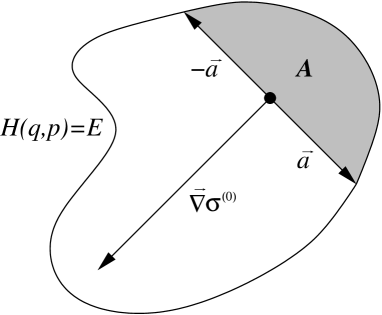
Figure 1: Determining the lowest order $\hbar$ contribution to the phase of the WF. The closed curve represents the manifold (curve) of constant energy. The gradient $\vec{\nabla}\sigma^{(0)}$ is orthogonal to the vector $\vec{a}$, with the the actual value of the phase $\sigma^{(0)}$ being given by the area $A$ (see the main text for details).

The lowest, zero order $\hbar$ contribution is an expression that looks trivial at first, yet, however, it is quite involved,

$$(H)_{2}=E,$$ (64)

as it gives the pair of equations

$$H\left(q_{1}^{(0)}\pm\frac{1}{2}\left(\frac{\partial\sigma^{(0)}}{\partial p}\right)_{1},\ p_{1}^{(0)}\mp\frac{1}{2}\left(\frac{\partial\sigma^{(0)}}{\partial q}\right)_{1}\right)=E.$$ (65)

We can use this pair of equations to determine the local gradient of the leading order phase contribution. It is determined by the chord that can be spanned between two points on the curve (manifold) of the constant energy, $H(q,p)=E$, for which $(q_{1},p_{1})$ is the center. The size of the gradient is equal to the length of this chord, while at the same time the gradient is orthogonal to it (see figure 1).

Using this gradient we may also determine the actual value of the function $\sigma^{(0)}$. The easiest way to do this is to find all such chords that are parallel to the one corresponding to the chosen point $(q_{1},p_{1})$ and lie between this point and the energy surface. The centers of these chords form a path ${\bf s}$ in the phase space that starts on the energy surface and ends in the point $(q_{1},p_{1})$. The change of phase along this path is given by

$$\sigma^{(0)}=\int\vec{\nabla}\sigma^{(0)}\cdot d{\bf s}=\int l({\bf s})dh=A,$$ (66)

where $l$ denotes the length of the chord that corresponds to the given point ${\bf s}$ and $dh$ is the component of $d{\bf s}$ that is perpendicular to the chord. The value of this integral is $A$, which gives exactly the area of the region between the chord around a chosen point and the curve of constant energy. This result is the same as obtained by Berry (1977a) where the phase of the WF was determined using the leading semiclassical approximation for the WF.

The above equations typically give a pair of solutions. By properly connecting these solutions at the caustics along with taking into account higher order corrections leads to the quantization conditions and subsequent determination of the semiclassical energies (see Berry 1977a for details).

Let us now consider the higher order $\hbar$ equations. All the terms that contribute in the linear order of $\hbar$ give the pair of equations

$$i\hbar\left[\mp\frac{1}{2}\left(\left(\frac{\partial H}{\partial p}\right)_{2}\left(\frac{\partial\sigma^{(1)}}{\partial q}\right)_{1}-\left(\frac{\partial H}{\partial q}\right)_{2}\left(\frac{\partial\sigma^{(1)}}{\partial p}\right)_{1}\right)\right.$$

$$-\left.\frac{1}{8}\left(\left(\frac{\partial^{2}H}{\partial p^{2}}\right)_{2}\left(\frac{\partial^{2}\sigma^{(0)}}{\partial q^{2}}\right)_{1}+\left(\frac{\partial^{2}H}{\partial q^{2}}\right)_{2}\left(\frac{\partial^{2}\sigma^{(0)}}{\partial p^{2}}\right)_{1}\right)\right]=0,$$ (67)

while the next order is already a more involved expression

$$-\hbar^{2}\left[\mp\frac{1}{2}\left(\left(\frac{\partial H}{\partial p}\right)_{2}\left(\frac{\partial\sigma^{(2)}}{\partial q}\right)_{1}-\left(\frac{\partial H}{\partial q}\right)_{2}\left(\frac{\partial\sigma^{(2)}}{\partial p}\right)_{1}\right)\right.$$ (68)

$$-\frac{1}{8}\left(\left(\frac{\partial^{2}H}{\partial p^{2}}\right)_{2}\left(\frac{\partial^{2}\sigma^{(1)}}{\partial q^{2}}\right)_{1}+\left(\frac{\partial^{2}H}{\partial q^{2}}\right)_{2}\left(\frac{\partial^{2}\sigma^{(1)}}{\partial p^{2}}\right)_{1}\right)$$

$$\mp\frac{1}{48}\left(\left(\frac{\partial^{3}H}{\partial p^{3}}\right)_{2}\left(\frac{\partial^{3}\sigma^{(0)}}{\partial q^{3}}\right)_{1}-\left(\frac{\partial^{3}H}{\partial q^{3}}\right)_{2}\left(\frac{\partial^{3}\sigma^{(0)}}{\partial p^{3}}\right)_{1}\right)$$

$$+\frac{1}{8}\left(\left(\frac{\partial^{2}H}{\partial p^{2}}\right)_{2}\left(\left(\frac{\partial\sigma^{(1)}}{\partial q}\right)_{1}\right)^{2}+\left(\frac{\partial^{2}H}{\partial q^{2}}\right)_{2}\left(\left(\frac{\partial\sigma^{(1)}}{\partial p}\right)_{1}\right)^{2}\right)$$

$$\pm\frac{1}{32}\left(\left(\frac{\partial^{3}H}{\partial p^{3}}\right)_{2}\left(\frac{\partial^{2}\sigma^{(1)}}{\partial q^{2}}\right)_{1}\left(\frac{\partial\sigma^{(1)}}{\partial q}\right)_{1}-\left(\frac{\partial^{3}H}{\partial q^{3}}\right)_{2}\left(\frac{\partial^{2}\sigma^{(1)}}{\partial p^{2}}\right)_{1}\left(\frac{\partial\sigma^{(1)}}{\partial p}\right)_{1}\right)$$

$$+\left.\frac{1}{128}\left(\left(\frac{\partial^{4}H}{\partial p^{4}}\right)_{2}\left(\left(\frac{\partial^{2}\sigma^{(0)}}{\partial q^{2}}\right)_{1}\right)^{2}+\left(\frac{\partial^{4}H}{\partial q^{4}}\right)_{2}\left(\left(\frac{\partial^{2}\sigma^{(0)}}{\partial p^{2}}\right)_{1}\right)^{2}\right)\right]=0.$$

Equations that correspond to higher orders are quite similar, and they contain higher orders of derivatives of both $H$ and $\sigma^{(n)}$, while at the same time higher order products of $\sigma_{1}^{(n)}$ are involved.

4 Harmonic oscillator

As is almost customary in quantum mechanics, the test example for any new method is the harmonic oscillator. By properly scaling the coordinates the Hamiltonian can be written as

$$H(q,p)=\frac{1}{2}\omega\left(p^{2}+q^{2}\right).$$ (69)

As the Hamiltonian is quadratic in both the momentum and the coordinate, only those terms of the equation (63) can feature in its analysis that contain at most the second order derivative of the Hamiltonian and, consequently, the phase $\sigma$. At the same time the Hamiltonian is symmetric with respect to rotations around the phase space origin, and the same is true of the solutions

$$\sigma^{(n)}=\sigma^{(n)}(r)$$ (70)

which depend only on the distance

$$r=\sqrt{q^{2}+p^{2}}$$ (71)

from the phase space origin.

Apart from the lowest order in the expansion over the powers of $\hbar$, the proper equations for all orders $n\geq 1$ in the $\hbar$ expansion for this system are given by

$$\frac{1}{2}\hbar^{n}\omega\left(\gamma(r)\frac{\partial\sigma^{(n)}}{\partial r}\right)-\frac{1}{8}\hbar^{n}\omega\left(\frac{\partial^{2}\sigma^{(n-1)}}{\partial r^{2}}+\frac{1}{r}\frac{\partial\sigma^{(n-1)}}{\partial r}\right)+\frac{1}{8}\hbar^{n}\omega\left(\sum_{m=1}^{n-1}\frac{\partial\sigma^{(m)}}{\partial r}\frac{\partial\sigma^{(n-m)}}{\partial r}\right)=0,$$ (72)

which is obtained from the pair of equations (63) by rewriting them in the radial coordinates, where the fact that the solution is symmetric with respect to rotations reduces both of these equations to the expression above. We also introduced

$$\gamma(r)=\left(\frac{2E}{\omega}-r^{2}\right)^{\frac{1}{2}}.$$ (73)

For the lowest order solution we use the equation (65) to obtain

$$\frac{\partial\sigma^{(0)}}{\partial r}=2\gamma(r).$$ (74)

The next order in the expansion of $\sigma$ over powers of $\hbar$ is obtained by the equation (72), which gives

$$\frac{\partial\sigma^{(1)}}{\partial r}=\frac{1}{2}\left(\frac{\gamma^{{}^{\prime}}(r)}{\gamma(r)}+\frac{1}{r}\right),$$ (75)

and, after integration,

$$\sigma^{(1)}=\frac{1}{2}\left[\ln(\gamma(r))+\ln(r)\right]$$ (76)

In the figure 3 we show the semiclassical approximations to the WFs (dashed) for various eigenstates by using the two contributions above along with the exact solutions (full lines)

$$W_{N}(r)=\frac{1}{\pi\hbar}\exp\left(-\frac{r^{2}}{\hbar}\right)L_{N}\left(\frac{2r^{2}}{\hbar}\right)$$ (77)

where $L_{N}$ represents the Laguerre polynomial of order $N$. We used the relationship (Robnik 1998)

$$\int dqdp~{}W^{2}(q,p)=\frac{1}{2\pi\hbar}.$$ (78)

to normalize the WFs.

Figure 2: We show the complex plane of the variable $r$. With the thick line we depict the cut in the complex plane that needs to be taken out of the area of definition of the phase derivative, $\sigma^{\prime}$, in order for it to be defined uniquely. We also show the contour ${\cal P}$ that goes around the singularities in the points $r=\{0,\pm\kappa\}$, where $\kappa=\sqrt{2E/\omega}$, and from which the quantization condition is determined

To find these approximate solutions as well as to perform further analysis the solution in the whole complex plane needs to be carefully defined. Due to the singularities of $\partial\sigma^{(0)}/\partial r$ and $\partial\sigma^{\prime(1)}/\partial r$ in the points $r=\{0,\pm\sqrt{2E/\omega}\}$ and the fractional power expressions in both of them we can only make these derivatives uniquely defined on the whole complex plane with the cut as shown in the figure 2. This cut, on the other hand, just coincides with the main domain on which we seek the solution. Therefore we obtain two contributions on this cut that are the limits of the expressions as obtained by the limit of approaching the cut from the upper or lower side, and therefore these expressions correspond to various sections of the path ${\cal P}$. It is interesting to note that this cut is actually essential if we want the whole solution to be made real. Therefore we used the two branches when constructing the total solution, which are obtained by taking the positive and negative value of the square root in the definition of $\gamma(r)$ which then makes the total result real. By using both contributions we may write the approximation to our Wigner function as

$$W(r)=A\cos\left(\frac{\sigma^{(0)}}{\hbar}+\theta\right)\exp(-\sigma^{(1)}),$$ (79)

where $A$ is a real constant. Evaluating the integral of the equation (78) therefore gives

$$\frac{1}{2\pi\hbar}=\int dqdp~{}W^{2}(q,p)\approx\frac{A^{2}}{2}\int dqdp~{}\exp(-2\sigma^{(1)}),$$ (80)

where the value of the square of the trigonometric function was replaced by its average which can indeed be done in the semiclassical limit $\hbar\to 0$ where this function is rapidly oscillating. In our case this gives

$$\int dqdp~{}\exp(-2\sigma^{(1)})=2\pi\int_{0}^{\sqrt{\frac{2E}{\omega}}}r~{}dr~{}\frac{1}{\gamma(r)r}=\pi^{2}$$ (81)

and therefore

$$A=\frac{1}{\sqrt{\pi^{3}\hbar}}.$$ (82)

We still need to determine the phase shift $\theta$, which is altered every time we encounter a singularity of $\partial\sigma^{(1)}/\partial r$ when traversing the path ${\cal P}$ as shown in the figure 2. Although the expression (76) tells us that the weight of the logarithmic contribution (which are responsible for the phase shifts) when traversing the point $0$ is twice as strong as that at the other singular points, we also need to take into account that traversing the path ${\cal P}$ we only do a half of the full enclosure of this singular point. Upon encountering any singularity along the contour ${\cal P}$ we therefore need to shift the phase by $-\pi/2$.

If at the same time we demand that the total phase upon the full traversal of the contour ${\cal P}$ must change by an integer multiple of $2\pi$, namely $2\pi M$, as the WF, which is exponentially dependent upon this phase, must be singlevalued, this leads to the quantization condition which will be given in full detail later. The difference is that we now only take into account the two lowest contributions of the expansion of the phase with respect to $\hbar$, although this already gives the exact result for the eigenenergies in our example. For odd $M$ it can be shown that we obtain semiclassical approximations for the WFs that are odd with respect to the reflection of $r$, which, however, contradicts the initial observation that the WFs must be invariant with respect to rotations around the phase space origin. For the even solutions ($M=2N$), on the other hand, we find that the phase shift in the expression (79) needs to be $\theta=-\pi/4$ for $r>0$ if $\sigma^{(0)}(r=0)=0$ is chosen. This yields the explicit expression of equation (79),

$$W_{N}(r)=\frac{(-1)^{N}}{\pi\hbar\sqrt{\pi y\sqrt{2N+1-y^{2}}}}\sin\left(y\sqrt{2N+1-y^{2}}-\right.$$

$$\left.-(2N+1)\arccos\left(\frac{y}{\sqrt{2N+1}}\right)+\frac{3\pi}{4}\right);\ \ r=\sqrt{\hbar}y$$ (83)

for $0<y<\sqrt{2N+1}$. This is exactly the result one would obtain by approximating the exact solution (77) using the large $N$ approximation for the expression $\exp(-y^{2}/2)L_{N}(y^{2})$ as found in (Szegö 1959).

Figure 3: A comparison of the semiclassical (dashed) and the exact (full line) WFs for various quantum numbers $N$, where we set $\hbar=\omega=1$. We used the first two terms in the $\hbar$ expansion of the phase to construct the semiclassical solutions.

This now completes our approximate treatment of the WFs for the harmonic oscillator, namely the two lowest orders, and now we turn to the exact treatment of the energy spectrum by considering all orders. By using a straightforward yet lengthy procedure of induction it is easy enough to show that the expression below, when inserted into (72), gives the correct solution to the problem,

$$\frac{\partial\sigma^{(n)}}{\partial r}=\omega\frac{\sum_{p=0}^{n}\alpha_{p}^{(n)}E^{n-p}(\omega r^{2})^{p}}{r^{n}\left(\frac{2E}{\omega}-r^{2}\right)^{\frac{3n-1}{2}}},$$ (84)

where $\alpha_{p}^{(n)}$ are unknown rational coefficients, except for $n=0,1$, where they are fixed by (74,75).

We may now try to calculate the spectrum. We obtain it by taking a certain energy $E$ in the above equations and then trying to find such a value $E$ so that the WF

$$\rho=\exp\left(i\frac{\sigma}{\hbar}\right)$$ (85)

is singlevalued. This does not necessarily mean that the value of the phase ${\sigma}/{\hbar}$ needs to be singlevalued, as it may change by an integer multiple of $2\pi$ when traversing any closed path in the complex plane without changing the value of $\rho$ after such a traversal.

It is interesting to note that using the classical WKB method to determine the eigenfunctions we may not directly link the condition of singlevaluedness to the condition of the solutions being square integrable. Yet the singlevaluedness condition yields the correct values for eigenenergies in systems that are exactly quantum solvable. Therefore the question can be posed whether the two conditions are equivalent or does this only apply to the solvable systems that usually possess some other special properties like solvability by the factorization method (Infeld and Hull 1951) or other (Cooper et al1995, Robnik and Salasnich 1997a, 1997b, Robnik and Romanovski 2000a, 2000b, Romanovski and Robnik 2000). For most of them we may find the appropriate quantum canonical transformations (Lahiri, Ghosh and Kar 1998, Veble 2001). As we will see, using the singlevaluedness condition yields the proper solution in our case as well.

Let us now choose the closed path ${\cal P}$ in the complex $r$ plane as given in figure 2 that encloses all the singularities of our problem. These are found in the points $r=\{0,\pm\sqrt{\frac{2E}{\omega}}\}$. The change of phase along this path,

$$\Delta\varphi=\frac{1}{\hbar}\oint_{\cal P}\sigma^{\prime}dr,$$ (86)

is given by the residuum of $\sigma^{\prime}$ at infinity. We obtain it by rewriting equation (84) as

$$\frac{\partial\sigma^{(n)}}{\partial r}=\omega\frac{\sum_{p=0}^{n}\alpha_{p}^{(n)}E^{n-p}(\omega r^{2})^{p}}{r^{n}\left(-r^{2}\right)^{\frac{3n-1}{2}}}\left(1+\frac{3n-1}{2}\frac{2E}{\omega r^{2}}+\ldots\right).$$ (87)

The leading term of such an asymptotic series is of the order $r^{-2n+1}$, with all the other terms comprising a higher negative power of $r$. As the residuum is given by the prefactor to the term containing $r^{-1}$, the above expression can have a nonzero residuum only for $n=0,1$. By taking into account equations (74) and (75), the evaluation of these residua therefore yields

$$\Delta\varphi={2\pi}\left[\frac{2E}{\hbar\omega}-1\right].$$ (88)

By specifying that the above change of phase needs to be an integer multiple of $2\pi$ we obtain the quantization condition for the energy

$$E=\hbar\omega\left[\frac{M}{2}+\frac{1}{2}\right],$$ (89)

where $M$ is a nonnegative number. These solutions, however, also contain those that yield WFs that are odd with respect to reflection of the $r$ coordinate. Since the proper solutions need to be invariant with respect to rotations around the phase space origin, only the even solutions are the proper ones. This leads to $M=2N$ and therefore

$$E=\hbar\omega\left[N+\frac{1}{2}\right].$$ (90)

By constructing the full semiclassical WFs we therefore solved the problem of the harmonic oscillator to all orders of $\hbar$ without referring to the actual wavefunctions. A similar analysis for the infinite potential well (1-dim box potential) is in progress (Veble 2001,2002)

5 Summary and conclusion

By devising a full semiclassical analysis of WFs we managed to rewrite quantum mechanics, that is typically considered in either only the momentum or coordinate representation, into an independent full phase space formalism. We obtained the full semiclassical equations to all orders of $\hbar$ for these functions. This enabled us to solve the problem of the harmonic oscillator as an example.

It is easy enough to generalize the equations themselves to more than one dimension. The problems arise when trying to solve for the main order contribution, as the mere condition of the appropriate chords lying on the energy surface yields infinitely many solutions. We need to take other conditions such as the singlevaluedness of the WFs with respect to all traversals in the phase space into account, and this is far from trivial to implement. Most likely such a procedure, if it is found, can function well only in classically integrable systems, or possibly for the regular states in the mixed systems, as nonintegrability and the chaotic motion associated with it break the ordered structure of the classical phase space which is most likely necessary for the generalization of the above procedure to work. Finding the extension of the approach to more than one degree of freedom is therefore the main goal of the work to follow.

References

References

• [1] Berry M 1977a Philosophical Transactions of the Royal Society of London A, 287 237
• [2] Berry M V 1977b, J. Phys. A: Math. Gen. 10 2083
• [3] Cooper F, Khare A and Sukhatme U 1995 Phys. Rep. 251 267-385
• [4] Curtright T, Fairlie D and Cosmas Z 1998 Physical Review D 5802 5002
• [5] Heller E J 1976 Jour. Chem. Phys. 65 (4) 1289
• [6] Heller E J 1977 Jour. Chem. Phys. 67 3339
• [7] Infeld L and Hull T E 1951 Rev. Mod. Phys. 23 21-68
• [8] Lahiri A, Ghosh G in Kar T M 1998 Physics Letters A 238 239-243
• [9] Osborn T A in Molzahn F H 1995 Ann. Phys. - New York 241 (1) 79
• [10] Ozorio de Almeida A M 1998 Physics Reports 295 265
• [11] Robnik M 1998 Nonlinear Phenomena in Complex Systems (Minsk) 1 1
• [12] Robnik M and Romanovski V 2000a J. Phys. A: Math. Gen. 33 5093-5104
• [13] Robnik M and Romanovski V 2000b Prog. Theor. Phys. Suppl. 139 399-403
• [14] Robnik M and Salasnich L 1997a J. Phys. A: Math. Gen. 30 1711-1718
• [15] Robnik M and Salasnich L 1997b J. Phys. A: Math. Gen. 30 1719-1729
• [16] Romanovski V and Robnik M 2000 J. Phys. A: Math. Gen. 33 8549-8557
• [17] Szegö G 1959 Orthogonal Polynomials (American Mathematical Society, New York)
• [18] Veble G 2001 Ph.D. Thesis (CAMTP, Universities of Maribor and Ljubljana)
• [19] Veble G 2002 In preparation