Dependence of heat transport on the strength and shear rate of prescribed circulating flows

Abstract

We study numerically the dependence of heat transport on the maximum velocity and shear rate of physical circulating flows, which are prescribed to have the key characteristics of the large-scale mean flow observed in turbulent convection. When the side-boundary thermal layer is thinner than the viscous boundary layer, the Nusselt number (Nu), which measures the heat transport, scales with the normalized shear rate to an exponent 1/3. On the other hand, when the side-boundary thermal layer is thicker, the dependence of Nu on the Peclet number, which measures the maximum velocity, or the normalized shear rate when the viscous boundary layer thickness is fixed, is generally not a power law. Scaling behavior is obtained only in an asymptotic regime. The relevance of our results to the problem of heat transport in turbulent convection is also discussed.

I Introduction

Turbulent Rayleigh-Bénard convection has been a system of much research interest. The system consists of a closed cell of fluid which is heated from below and cooled from above. When the applied temperature difference is large enough, the fluid moves and convection occurs. The flow state is characterized by the geometry of the cell and two dimensionless control parameters: the Rayleigh number Ra, which measures how much the fluid is driven and the Prandtl number Pr, which is the ratio of the diffusivities of momentum and heat of the fluid. The two parameters are defined by Ra $=\alpha g\Delta L^{3}/(\nu\kappa)$, and Pr $=\nu/\kappa$, where $\Delta$ is the maintained temperature difference, $L$ is the height of the cell, $g$ the acceleration due to gravity, and $\alpha$, $\nu$, and $\kappa$ are respectively the volume expansion coefficient, kinematic viscosity and thermal diffusivity of the fluid. When Ra is sufficiently large, the convection becomes turbulent.

Besides the issue of the statistical characteristics of the velocity and temperature fluctuations, it is of interest to understand the heat transport by the fluid, which is an overall response of the system. The heat transport is usually expressed as the dimensionless Nusselt number Nu, which is the ratio of the measured heat flux to the heat transported were there only conduction. Before the onset of convection, heat is transported only by conduction and Nu is identically equal to one. When convection occurs, heat is more effectively transported by the fluid due to its motion and Nu increases from 1. A major question is then to understand how Nu depends on Ra and Pr.

The work of Libchaber and coworkers on turbulent convection in low temperature helium gas[1, 2] showed that Nu has a simple power-law dependence on Ra:

$${\rm Nu}\sim{\rm Ra}^{\beta}$$ (1)

and the exponent $\beta$ is almost equal to $2/7$, which is different from $1/3$, the value that marginal stability arguments[3] would give. This result led to the development of several theories[2, 4, 5, 6] which all give $\beta=2/7$ but were based on rather different physical assumptions. In particular, the Chicago mixing-zone model [2] emphasizes the heat transport by the thermal plumes, the coherent structures observed in turbulent convection while the theory by Shraiman and Siggia[5] focuses on the effect of the shear of the large-scale mean flow on the heat transport (see e.g. Ref.[7] for a review). Recent experimental results appeared to further complicate the situation. Niemela et al.[8] reported a value of $\beta$ close to 0.31 for measurements in low temperature helium gas that cover a much larger range of Ra, from $10^{6}$ to $10^{17}$. Xu et al.[9] studied turbulent convection in acetone in several experimental cells of different aspect ratios and concluded that there is no significant range of Ra over which the scaling behavior Eq. (1) holds. Furthermore, they showed that for Ra $\geq 10^{7}$, the dependence of Nu on Ra can be represented by a combination of two power laws, which is consistent with a recent theory by Grossmann and Lohse[10, 11]. In Grossmann and Lohse’s theory, the viscous and thermal dissipation were decomposed into their bulk and boundary-layer contributions, and ten asymptotic regimes were obtained[11].

Another interesting feature observed in turbulent convection is the presence of a persistent large-scale mean flow which spans the whole experimental cell[12]. The maximum mean velocity of the flow was also found to scale as Ra to about 1/2[13]. The presence of a large-scale flow naturally induces an interaction between the top and bottom thermal boundary layers. Such an interaction was taken to be absent in the marginal stability arguments. One obvious effect of the velocity field, which satisfies the no-slip boundary condition, is that it produces a shear near the boundaries, which was first studied in Ref.[5].

In convection, the equations of motion are:

$${\displaystyle\partial{\vec{u}}\over\displaystyle\partial t}+{\vec{u}}\cdot{\vec{\nabla}}{\vec{u}}=-{\vec{\nabla}}p+\nu\nabla^{2}{\vec{u}}+g\alpha T\hat{z}$$ (3)

$${\displaystyle\partial T\over\displaystyle\partial t}+{\vec{u}}\cdot{\vec{\nabla}}T=\kappa\nabla^{2}T$$ (4)

$${\vec{\nabla}}\cdot{\vec{u}}=0$$ (5)

where ${\vec{u}}$ is the velocity field, $p$ the pressure divided by density and $T$ the temperature field, while $\hat{z}$ is the unit vector in the vertical direction. The velocity and temperature are thus coupled dynamically in a complicated fashion and have to be solved together. Physically, the velocity field is driven by the applied temperature difference. The flow in turn determines the temperature profile, and thus the heat transport, in a self-consistent manner.

To gain insights of the problem of heat transport in turbulent convection, we have turned to the simpler problem of heat transport by prescribed velocity fields that have features of the large-scale mean flow observed. The large-scale flow has two dominant features: (i) it is a circulating flow that spans the whole experimental cell and (ii) it generates a shear near the boundaries. In an earlier paper, Ching and Lo studied separately these two features and their effects on the heat transport[14]. They found that Nu scales with the Peclet number that measures the maximum velocity to an exponent 1/2 for a purely circulating flow and scales with the normalized shear rate to an exponent 1/3 for a pure shear.

Pure circulating or pure shear flows are, however, not physical fluid flows within a closed box. In this paper, we continue along these lines of thought and study the heat transport by physical velocity fields in a unit square cell that have both the circulating and the shear-generating features. We focus on the dependence of the heat transport on the maximum velocity and the shear rate of the flows. We first formulate our problem in Sec. II. Then we present our numerical results and discuss how these results can be understood in Sec. III. In Sec. IV, we further discuss how these results are relevant to the understanding of heat transport in turbulent convection. Finally, we end the paper with a summary and conclusions in Sec. V.

II The Problem

We solve the steady-state advection-diffusion equation

$${\vec{u}}(x,y)\cdot\vec{\nabla}T(x,y)=\kappa\nabla^{2}T(x,y)\$$ (6)

for a prescribed incompressible velocity field ${\vec{u}}(x,y)$ in a unit square cell: $0\leq x\leq L$ and $0\leq y\leq L$. A temperature difference of $\Delta$ is applied across the $y$-direction while no heat conduction is allowed across the $x$-direction. That is, the temperature field $T(x,y)$ satisfies the following boundary conditions:

$$T(x,y=0)=\Delta; T(x,y=L)=0$$ (7)

$${\partial T\over\partial x}(x=0,y) = {\partial T\over\partial x}(x=L,y)=0$$ (8)

For the velocity field, we take

$$u_{x}(x,y) = f(\tilde{x})f^{\prime}(\tilde{y})$$ (9)

$$u_{y}(x,y) = -f^{\prime}(\tilde{x})f(\tilde{y})$$ (10)

where $f$ is some function of $\tilde{x}\equiv x/L$ or $\tilde{y}\equiv y/L$ and ^′ is its derivative with respect to the argument. Thus, $\vec{u}$ is incompressible and separable in $x$ and $y$. To satisfy the no-slip boundary condition, we require

$$f(0)=f(1)=f^{\prime}(0)=f^{\prime}(1)=0$$ (11)

Moreover, for $\vec{u}$ to be a circulating flow, we require

$$f(\tilde{x})=f(1-\tilde{x})\qquad 0\leq\tilde{x}\leq 1$$ (12)

such that $u_{x}$ and $u_{y}$ are antisymmetric about $y=L/2$ and $x=L/2$ respectively. We have studied two forms of $f$. The first form is algebraic. When $f$ is algebraic, Eqs. (11) and (12) imply that $f(\tilde{x})={\tilde{x}}^{2}({\tilde{x}}-1)^{2}h(\tilde{x})$ with $h(\tilde{x})=h(1-\tilde{x})$. Thus we choose

$$f(\tilde{x})={\tilde{x}}^{2}({\tilde{x}}-1)^{2}(a\tilde{x}+b)[a(1-\tilde{x})+b]$$ (13)

where $a$ and $b$ are positive constants. Equation (13) is the simplest algebraic form that allows us to change both the circulating strength and the shear rate of the flow (see below). The other is an exponential form of $f$:

$$f(\tilde{x})=c(1-e^{-k\tilde{x}})^{2}[1-e^{-k(1-\tilde{x})}]^{2}$$ (14)

where $c$ and $k$ are positive constants. For $k\ll 1$, the exponential form reduces to the algebraic form with $a=0$ and $b^{2}=ck^{4}$. When $k$ is large, the velocity decays exponentially towards the center of the cell. We show the two velocity fields in Fig. 1.

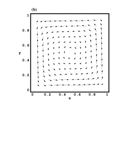
FIG. 1.: (a) The velocity field with an alegbraic $f$ given by Eq. (13) with $a=b=1$. The size of the arrow indicates the relative magnitude of the velocity. The contour $C$ that encloses the lower half of the unit square cell is also shown. (b) The velocity field with an exponential $f$ given by Eq. (14) with $c=1$ and $k=9$.

We characterize the velocity field by its maximum velocity $u_{0}$ and shear rate $\gamma$, which are defined by

$$u_{0} \equiv \max_{0\leq y\leq{L\over 2}}\,u_{x}(x={L\over 2},y)=\max_{0\leq x\leq{L\over 2}}\,-u_{y}(x,y={L\over 2})$$ (15)

$$\gamma \equiv {\partial u_{x}\over\partial y}(x={L\over 2},y)\bigg{|}_{y=0}=-{\partial u_{y}\over\partial x}(x,y={L\over 2})\bigg{|}_{x=0}$$ (16)

By varying the parameters $a$ and $b$ or $c$ and $k$, we can vary $u_{0}$ and $\gamma$ of the velocity fields.

From the solved temperature field, we can calculate the heat transport, which is the heat conducted across the boundary $y=0$. Nu is therefore the ratio of the average of the magnitude of the vertical temperature gradient over the boundary $y=0$ to $\Delta/L$:

$${\rm Nu}={\displaystyle\langle-{\partial T\over\partial y}\bigg{|}_{y=0}\rangle\over\displaystyle{\Delta\over L}}$$ (17)

Here $\langle\ldots\rangle$ is the average over $x$ from 0 to $L$. Our goal is to study the dependence of Nu on the Peclet number Pe $\equiv u_{0}L/\kappa$ and the normalized shear rate $\tilde{\gamma}\equiv\gamma L^{2}/\kappa$.

III Results and Discussions

We numerically solve $T(x,y)$ for the two forms of $f$. In Fig. 2, we show the vertical and horizontal temperature profiles $T(x=L/2,y)$ and $T(L-x,y=L/2)$. As was reported in turbulent convection experiments, the applied temperature difference concentrates in two narrow regions near the ‘bottom’ and ‘top’ boundaries $y=0$ and $y=L$ respectively. Interestingly, the circulation also induces a temperature difference between the two ‘side’ boundaries $x=0$ and $x=L$. For flows that are anticlockwise (see Fig. 1), the side $x=0$ is colder than the side $x=L$. The horizontal temperature profile $T(L-x,y=L/2)$ resembles the vertical one $T(x=L/2,y)$ in that it is almost constant = $\Delta/2$ except for two small regions near the sides. In these two small regions, it is approximately linear in $x$ except at the boundaries where the horizontal gradient vanishes. Hence, we approximate $T(x,y=L/2)$ by

$${T(x,y=L/2)\over\Delta/2}\approx\cases{1-\alpha\left(1-{x\over\ell}\right)&$0\leq x\leq\ell$\cr 1&$\ell<x<L-\ell$\cr 1+\alpha\left(1-{L-x\over\ell}\right)&$L-\ell\leq x\leq L$}$$ (18)

where $\alpha$ is about $0.5$ as shown in Fig. 3.

FIG. 2.: Typical vertical and horizontal temperature profiles $T(x=L/2,y)/\Delta$ (solid) and $T(L-x,y=L/2)/\Delta$ (dotted) as a function of $y/L$ and $x/L$ respectively.

FIG. 3.: The dependence of $\alpha$ on $\tilde{\gamma}$ for various values of $\lambda_{v}$: $\lambda_{v}/L=0.0167$ (circles), $\lambda_{v}/L=0.021$ (triangles), $\lambda_{v}/L=0.028$ (stars), $\lambda_{v}/L=0.070$ (squares), $\lambda_{v}/L=0.088$ (plusses), $\lambda_{v}/L=0.096$ (diamonds), $\lambda_{v}/L=0.108$ (crosses), and $\lambda_{v}/L=0.130$ (inverted triangles).

Thus, there are also two thermal boundary layers of thickness $\ell$ at the ‘side’ boundaries. Furthermore, we find that Nu is given by $L/\ell$ up to a factor $d$:

$${\rm Nu}=d{L\over\ell}$$ (19)

where $d$ is weakly independent of $\tilde{\gamma}$ and approaches $0.8$ as the viscous boundary layer thickness $\lambda_{v}\equiv u_{0}/\gamma$ increases to 0.13 $L$ as shown in Fig. 4. Defining $\lambda_{T}=L/(2{\rm Nu})$ to be the average thickness of the thermal boundary layer at the top and bottom boundaries, we see that the $\ell=2d\lambda_{T}$. Thus, the side-wall thermal boundary layers are thicker than the top and bottom thermal boundary layers.

FIG. 4.: The dependence of $d$ on $\tilde{\gamma}$ for various values of $\lambda_{v}$ (same symbols as in Fig. 3).

We find that the functional form of Nu(Pe,$\tilde{\gamma}$) depends crucially on the relative sizes of $\lambda_{v}$ and $\ell$. For $\ell<\lambda_{v}$, Nu scales with the shear rate:

$${\rm Nu}=A{\tilde{\gamma}}^{1/3}\qquad{\rm for}\ \ell<\lambda_{v}$$ (20)

and the coefficient $A$ approaches 0.36 as $\lambda_{v}$ increases to 0.13 $L$ as shown in Fig. 5. For $\lambda_{v}<\ell$, we see in Fig. 6 that the dependence of Nu on Pe or $\tilde{\gamma}$ for fixed $\lambda_{v}$ is not a power law. For a short range of Pe or $\tilde{\gamma}$, the dependence might be described by an effective power law but the value of the effective exponent would depend on the range of Pe or $\tilde{\gamma}$ fitted.

We shall understand these results in the following. Since the velocity field is incompressible, Eq. (6) implies

$$\int_{C}\left(\vec{u}T-\kappa\vec{\nabla}T\right)\cdot\hat{n}dl=0$$ (21)

for any closed curve $C$ in the two-dimensional domain where $\hat{n}$ is an outward normal. Since we find that $|\partial T/\partial y|$ almost vanishes along $y=L/2$, we choose $C$ to enclose the lower half of the unit cell (see Fig. 1a). Together with Eq. (8) and the no-slip boundary condition, Eq. (21) then implies that

$${\rm Nu}\approx{L\over\kappa\Delta}\langle u_{y}(x,y={L\over 2})T(x,y={L\over 2})\rangle$$ (22)

Thus, we can estimate Nu by the heat transported across $y=L/2$. Using the antisymmetry of $u_{y}$ about $x=L/2$ and Eq. (18), we get

$$\langle u_{y}(x,y={L\over 2})T(x,y={L\over 2})\rangle$$ (23)

$$= {2\over L}\int_{0}^{\ell}u_{y}(x,y={L\over 2})\left[T(x,y={L\over 2})-{\Delta\over 2}\right]dx$$ (24)

$$\approx -{\alpha\Delta\over L}\int_{0}^{\ell}(1-{x\over\ell})u_{y}(x,y={L\over 2})dx$$ (25)

In the derivation of Eq. (25), we have assumed that the parameters of the velocity field are chosen such that $\ell<L/2$ as in physical situations. The heat transported across $y=L/2$ is, therefore, contributed mainly by two ‘jets’ of colder and hotter fluids moving down and up respectively along the two boundaries $x=0$ and $x=L$.

FIG. 5.: The dependence of Nu on $\tilde{\gamma}$ when $\ell<\lambda_{v}$ for various values of $\lambda_{v}$ (same symbols as in Fig. 3). In the inset, Nu${\tilde{\gamma}}^{-1/3}$ is plotted versus $\tilde{\gamma}$.

FIG. 6.: The dependence of Nu on $\tilde{\gamma}$ when $L/2\gg\ell>\lambda_{v}$ for various values of $\lambda_{v}$ (same symbols as in Fig. 3). We also compare our numerical results to Eq. (29) with $\lambda_{v}/L=1/60$, $\alpha=0.6$ and $d=0.9$ (solid line), and good agreement is found for $\ell<0.1L$ (data points on the right of the dashed line).

Using Eq. (16), we approximate $u_{y}$ by a linear function in $x$ for $x<\lambda_{v}$:

$$u_{y}(x,{L\over 2})=-\gamma x\qquad{\rm for}\ x<\lambda_{v}$$ (26)

Hence, Eqs. (19), (22) and (25) give

$${\rm Nu}\approx\left({\alpha d^{2}\over 6}\right)^{1/3}{\tilde{\gamma}}^{1/3}\qquad{\rm for}\ \ell<\lambda_{v}$$ (27)

In Fig. 7, we compare our estimated values of the coefficient $(\alpha d^{2}/6)^{1/3}$ with the computed values of $A$. It can be seen that the two values agree within an error of 7%. Moreover, the agreement is better for larger $\lambda_{v}$, as expected since the linear approximation Eq. (26) works better for $0<x\leq\ell$ for larger $\lambda_{v}$.

FIG. 7.: Comparison of the estimated values of the coefficient $(\alpha d^{2}/6)^{1/3}$ (circles) with the computed values of $A$ (squares).

For $\ell>\lambda_{v}$, we need $u_{y}$ beyond the region where a linear approximation holds. As a first approximation, we take

$$-u_{y}(x,y={L\over 2})\approx\cases{\gamma x&$x<\lambda_{v}$\cr u_{0}&$\lambda_{v}\leq x\leq\ell$}$$ (28)

That is, we approximate the large-scale flow by a shear near the boundaries then followed by a band of circulation at the maximum velocity. As $u_{y}$ has to decay to zero towards the center of the cell, we expect the approximation Eq. (28) to work only for $\lambda_{v}<\ell\ll L/2$.

Using Eqs. (22), (25) and (28), we get a quadratic equation for Nu. Solving which gives

$${\rm Nu}={\sqrt{2\alpha d{\rm Pe}-(\alpha^{2}/12){\rm Pe}^{4}{\tilde{\gamma}}^{-2}}-(\alpha/2){\rm Pe}^{2}{\tilde{\gamma}}^{-1}\over 2\left(1-{\alpha\over 6d}{\rm Pe}^{3}{\tilde{\gamma}}^{-2}\right)}$$ (29)

for $L/2\gg\ell>\lambda_{v}$. Thus, Nu does not have a power-law dependence on Pe nor $\tilde{\gamma}$. Physically, this is because we generally cannot neglect the effect of the shear even when the edge of the side-wall thermal boundary layer is located at the band of maximum velocity of the large-scale flow. It is only in the limit Pe${}^{3/2}/\tilde{\gamma}\ll 1$ that Nu $\sim$ Pe^1/2. Away from this asymptotic regime, Nu might be represented by an effective power law on Pe or $\tilde{\gamma}$ for fixed $\lambda_{v}$ but the value of the effective exponent would depend on the range of Pe or $\tilde{\gamma}$ fitted. In Fig. 6, we compare the numerical results to Eq. (29) with $\lambda_{v}/L=1/60$, $\alpha=0.6$ and $d=0.9$. The agreement is not too bad for $\lambda_{v}<\ell<0.1L$ given that our approximation of $u_{y}$ being constant beyond the shear layer is rather crude.

IV Relevance to Turbulent Convection

In turbulent convection, the heat transport is due both to the large-scale mean flow and the fluctuating part of the velocity field. Our present work provides insights only to the heat transport by the large-scale mean flow. It is illuminating to see what results would be inferred if we neglect the effect of the fluctuating part of the velocity field.

Depending on the type of the viscous boundary layer, the strength and the shear rate would be related to each other. For example, if we follow Grossmann and Lohse to assume that viscous boundary layer is of Blasius type[15]: $\lambda_{v}/L\sim\sqrt{{\rm Pe}/{\rm Pr}}$ for moderate values of Pr[10] and that $\lambda_{v}\sim L$ for very large values of Pr[11], then

$$\tilde{\gamma}\sim\cases{{\rm Pe}^{3/2}{\rm Pr}^{-1/2}&{\rm moderate \ Pr}\cr{\rm Pe}&{\rm very \ large \ Pr}}$$ (30)

Our results Eqs. (27) and (29) would thus give Nu as a function of Pe and Pr:

$${\rm Nu}\approx\cases{\left({\alpha d^{2}\over 6}\right)^{1/3}{\rm Pe}^{1/2}{\rm Pr}^{-1/6}&{\rm moderate \ Pr}\cr\left({\alpha d^{2}\over 6}\right)^{1/3}{\rm Pe}^{1/3}&{\rm very \ large \ Pr}}$$ (31)

for $\ell<\lambda_{v}$ and

$${\rm Nu}\approx g({\rm Pr}){\rm Pe}^{1/2}$$ (32)

for $L/2\gg\ell>\lambda_{v}$ with

$$g({\rm Pr})={\sqrt{\alpha d-\alpha^{2}{\rm Pr}/12}-\alpha{\rm Pr}^{1/2}/2\over 2[1-\alpha{\rm Pr}/(6d)]}$$ (33)

We emphasize that the non-power-law dependence on Pr for $\ell>\lambda_{v}$ echoes that the effect of the shear cannot generally be neglected even when the edge of the side-wall thermal boundary layer is located at the band of the maximum velocity of the large-scale flow.

Next, we make use of a rigorous relation between the viscous dissipation and Nu and Ra, which is derivable from the equations of motion[5, 7]:

$$\langle\langle[\partial_{i}u_{j}({\bf x},t)]^{2}\rangle\rangle={\kappa^{2}\over L^{4}}({\rm Nu}-1){\rm Ra}$$ (34)

where $\langle\langle\ldots\rangle\rangle$ is an average over space x and time $t$. Neglecting the contribution from the fluctuating part of the velocity field to the viscous dissipation, we get

$$\tilde{\gamma}{\rm Pe}\sim{\rm NuRa}$$ (35)

for Nu $\gg 1$. Using Eqs. (30), (31), (32) and (35), we finally get

$${\rm Nu}\sim{\rm Pr}^{-1/12}{\rm Ra}^{1/4},\ \ {\rm Pe}\sim{\rm Pr}^{1/6}{\rm Ra}^{1/2}$$ (36)

$${\rm Nu}\sim{\rm Ra}^{1/5},\ \ {\rm Pe}\sim{\rm Ra}^{3/5}$$ (37)

for $\ell<\lambda_{v}$ respectively for moderate and very large values of Pr, and

$${\rm Nu} \sim g({\rm Pr})^{5/4}{\rm Pr}^{1/8}{\rm Ra}^{1/4}$$ (38)

$${\rm Pe} \sim g({\rm Pr})^{1/2}{\rm Pr}^{1/4}{\rm Ra}^{1/2}$$ (39)

for $L/2\gg\ell>\lambda_{v}$. The results Eqs. (36), (37), and (39), except for the non-power-law dependence on Pr in Eq. (39), resemble those obtained by Grossmann and Lohse[10], respectively for regimes $I_{l}$, $I_{\infty}^{<}$, and $I_{u}$, in which they took the boundary layer to dominate both the viscous and thermal dissipation.

V Summary and Conclusions

In this paper, we have studied the heat transport by physical fluid flows whose velocity fields are prescribed to have both the two key characteristics of the large-scale mean flow observed in turbulent convection. The velocity fields that we have chosen are separable and incompressible circulating flows in a unit square cell. Satisfying the no-slip boundary condition, they also generate a shear near the boundaries. Overall, they are approximately a shear near the boundaries, almost constant with the maximum strength of circulation for a finite band, and then a decay towards the center of the cell. We focus on the functional dependence of Nu on Pe measuring the maximums strength of circulation and the normalized shear rate $\tilde{\gamma}$ that characterize the velocity fields.

We have shown that Nu can be estimated by the heat transported across the mid-height of the unit square cell, which is in turn contributed mainly by two jets of hotter and colder fluids moving up and down the two sides. These two jets are confined to two narrow regions. That is, the velocity field also induces two thermal boundary layers at the side boundaries. These side-boundary thermal layers are thicker than those at the top and bottom boundaries. It is then clear that the functional form of Nu(Pe,$\tilde{\gamma}$) depends crucially on the relative sizes of the viscous boundary layer thickness $\lambda_{v}$ and the thickness of the thermal boundary layers at the side boundaries $\ell$. When $\ell<\lambda_{v}$, that is, the edge of the side-wall thermal boundary layer falls within the shear region of the large-scale flow, Nu scales with $\tilde{\gamma}$ to 1/3 and is very weakly dependent on $\lambda_{v}$ or Pe. When $\ell>\lambda_{v}$ and the edge of the side-wall thermal boundary layer falls within the band of circulation with maximum strength, there is still contribution to the heat transport by the shear and Nu depends on both Pe and $\tilde{\gamma}$. The dependence is generally not a power law and scaling behavior is obtained only in the asymptotic regime Pe${}^{3/2}/\tilde{\gamma}\ll 1$.

We have further discussed how our results are relevant to the problem of heat transport in turbulent convection. In turbulent convection, the heat transport is due both to the large-scale mean flow and the fluctuating part of the velocity field. Neglecting the effect of the fluctuating part of the velocity field, our results lead to results resembling those obtained by Grossmann and Lohse[10, 11] when they took the boundary layer to dominate both the viscous and thermal dissipation. It is not surprising that the boundary layer dominating the viscous dissipation is the same as the large-scale mean flow dominating the viscous dissipation since the gradient of the large-scale mean flow, which contributes to the viscous dissipation, concentrates in the boundary. Our finding thus suggests that whether the boundary layer or the bulk dominates the thermal dissipation is physically equivalent to whether the large-scale mean flow or the fluctuating part of the velocity field dominates the heat transport.

- [1] F. Heslot, B. Castaing, and A. Libchaber, Phys. Rev. A 36, 5870 (1987).
- [2] B. Castaing, G. Gunaratne, F. Heslot, L. Kadanaoff, A. Libchaber, S. Thomae, X.Z. Wu, S. Zaleski, and G. Zanetti, J. Fluid Mech. 204, 1 (1989).
- [3] See E.A. Spiegel, Ann. Rev. Astron. Astrophys. 9, 323 (1971); W. V. R. Malkus, Proc. R. Soc. London, Ser. A 225, 196 (1954); L. N. Howard, J. Fluid Mech. 17, 405 (1963).
- [4] Z.-S. She, Phys. Fluids A 1, 911 (1989).
- [5] B. I. Shraiman and E. D. Siggia, Phys. Rev. A 42, 3650 (1990).
- [6] S. Cioni, S. Ciliberto, and J. Sommeria, J. Fluid Mech. 335, 11 (1997).
- [7] E.D. Siggia, Ann. Rev. Fluid Mech. 26, 137 (1994), and references therein.
- [8] J.J. Niemela, L. Skrbek, K. R. Sreenivasan, and R. J. Donnelly, Nature 404, 837 (2000).
- [9] X. Xu, K. M.S. Bajaj, and G. Ahlers, Phys. Rev. Lett. 84, 4357 (2000).
- [10] S. Grossmann and D. Lohse, J. Fluid Mech. 407, 27 (2000).
- [11] S. Grossmann and D. Lohse, Phys. Rev. Lett. 86, 3316 (2001).
- [12] R. Krishnamurti and L.N. Howard, Proc. Nat. Acad. Sci. 78, 1981 (1981); M. Sano, X.Z. Wu, and A. Libchaber, Phys. Rev. A 40, 6421 (1989).
- [13] X.-Z. Wu, Ph.D. thesis, University of Chicago (1991).
- [14] Emily S.C. Ching and K.F. Lo, Phys. Rev. E 64, 046302 (2001).
- [15] L.D. Landau and E.M. Lifshitz, Fluid Mechanics (Pergamon Press, Oxford, 1987).