Localized Perturbations of Integrable Systems

Abstract

The statistics of energy levels of a rectangular billiard, that is perturbed by a strong localized potential, are studied analytically and numerically, when this perturbation is at the center or at a typical position. Different results are found for these two types of positions. If the scatterer is at the center, the symmetry leads to additional contributions, some of them are related to the angular dependence of the potential. The limit of the $\delta$-like scatterer is obtained explicitly. The form factor, that is the Fourier transform of the energy-energy correlation function, is calculated analytically, in the framework of the semiclassical geometrical theory of diffraction, and numerically. Contributions of classical orbits that are non diagonal are calculated and are found to be essential.

The distribution of energy levels exhibits a high degree of universality and is a central subject in the field of “Quantum Chaos” haakebook ; LH89 . For systems that are chaotic in the classical limit the statistics are of Random Matrix Theory (RMT)) bohigas84 , while for typical integrable systems the level distribution satisfies Poissonian statistics BT77 . In the semiclassical regime this universal behavior holds for a wide range in energy. There are also regimes of energy where spectral correlations related to periodic orbits are important berry85 ; AAA95 . In intermediate situations such a high degree of universality in not found. For mixed systems, where in some parts of phase space the motion is chaotic and in other parts it is regular, the statistics exhibit some general features berry84a ; izrailev88 . Another type of intermediate behavior may be found for integrable systems perturbed by singularities of spatial extension that is much smaller then the wavelength of the quantum particle. Examples of relevant systems are billiards with flux lines, sharp corners and $\delta$-like interactions seba90 ; bogomolny99E ; bogomolny01b . Here we report results obtained for a rectangular billiard perturbed by a $\delta$-like impurity long , known as the Šeba billiard seba90 . Some of these results can alternatively be concluded from a recent general formulation by Bogomolny and Giraud BG .

The interest in billiards of various types is primarily theoretical since it is relatively easy to analyze them analytically and numerically. Billiards were studied also experimentally for electrons marcus92 , microwaves stockmann90 and for laser cooled atoms davidson . We hope that in the future, perturbations of the type discussed in the present work will also be introduced experimentally.

Trace formulas that express the quantum density of states in the semiclassical limit as sums over classical periodic orbits were derived for chaotic gutz67 ; gutzwiller and integrable BT-I systems. For perturbations smaller than the wavelength, standard semiclassical theory used in the derivation of these formulas fails and diffraction effects have to be taken into account. This can be done in the framework of the Geometrical Theory of Diffraction (GTD) keller62 . In this approximation, which is valid far from the perturbation, the Green’s function for the system (without the boundary) is given by $G(k;{\bf r},{\bf r^{\prime}})\simeq G_{0}(k;{\bf r},{\bf r^{\prime}})+G_{0}(k;{\bf r},{\bf r}_{0})D(\theta,\theta^{\prime})G_{0}(k;{\bf r}_{0},{\bf r^{\prime}})$, where $\theta$ and $\theta^{\prime}$ denote the directions of ${\bf r}-{\bf r}_{0}$ and ${\bf r}_{0}-{\bf r^{\prime}}$ respectively and $G_{0}$ is the free Green’s function. The diffraction constant, $D$, describes the scattering from the perturbation. For the rectangular billiard with a $\delta$-like perturbation, that is subject of the present work, only diffraction effects are responsible for the deviations from the behavior of integrable systems. Therefore this is an ideal system for the exploration of such effects. Moreover for this problem the analytical and numerical calculations are relatively easy. The statistics depend on the location of the scatterer and on the boundary conditions bogomolny01b ; berkolaiko01 . This is in contrast to chaotic systems where the spectral statistics are not affected by such scatterers sieber99b .

The diagonal approximation berry85 , where only contributions from orbits with equal actions are considered is extensively used in the field of “Quantum Chaos”. It is not applicable for systems with localized perturbations. A method to take into account dominant non diagonal contributions, in integrable systems, was developed by Bogomolny bogomolny00b and will be used here.

In this work a rectangular billiard with sides $a_{x}$ and $a_{y}$, such that the aspect ratio is irrational, perturbed by a localized scatterer is studied. The scatterer is represented by a potential of typical size $a$ such that

$$U({\bf r})=\frac{1}{a^{2}}f\left(\frac{{\bf r}}{a}\right)$$ (1)

where $f({\bf y})$ is small where ${\bf y}$ is large.

The diffraction constant is the on shell matrix element of the ${\bf T}$ matrix $D(\theta^{\prime},\theta)=\langle{\bf k}|{\bf T}(E)|{\bf q}\rangle$ where ${\bf k}$ is the outgoing momentum (in direction $\theta^{\prime}$) and ${\bf q}$ is the incoming momentum (in the direction $\theta$). The energies of the incoming and outgoing waves are equal, that is $k=q=\sqrt{E}$ (in units $\hbar=1$ and $m=\frac{1}{2}$ used in this letter). The Born series cannot be used to compute $D(\theta^{\prime},\theta)$ when $ka\ll 1$ since the free Green’s function diverges as $\ln ka$ at short distances. A method that is regular when $ka\ll 1$ was introduced by Noyce noyce65 . In this method the scattering in the forward direction is resummed noyce65 . It leads to a diffraction constant that is a ratio of series. The series in the numerator and in the denominator are expanded in the number of scattering events (just like the Born series). Every term in these series is then expanded for $ka\ll 1$ (up to terms of order $k^{2}a^{2}$) and both series are summed (with respect the number of scattering events) to give the angle dependent diffraction constant long

$$D(\theta^{\prime},\theta)\simeq C\left[\rule{0.0pt}{19.91692pt}1+i\frac{ka}{2}\left\{\left(e^{i\theta}-e^{i\theta^{\prime}}\right)M_{1}+c.c\right\}-k^{2}a^{2}\left(M_{0}+\left\{\left(e^{2i\theta}+e^{2i\theta^{\prime}}\right)M_{2}+c.c.\right\}-\!\!\!\sum_{c,d=-1,+1}\!\!\!M_{cd}e^{i(c\theta^{\prime}+d\theta)}\right)\right]$$ (2)

where

$$C\equiv\left(\frac{V(1)}{V_{0}}+\frac{i}{4}-\frac{1}{2\pi}\left[\gamma+\ln\left(\frac{ka}{2}\right)\right]+k^{2}a^{2}\frac{Q(1)}{V_{0}}\right)^{-1},$$ (3)

$c.c.$ denotes the complex conjugate, $\gamma$ is Euler’s constant and $V_{0}=\int d^{2}yf({\bf y})$. Also $V(1)$, $Q(1)$, $M_{0}$, $M_{1}$, $M_{2}$ and $M_{cd}$ are constants, independent of $\theta$, $\theta^{\prime}$, and $M_{1}$, $M_{2}$ and $M_{cd}$ depend logarithmically on $ka$. These constants, given by series of integrals, involving the potential (1), were calculated in long .

In the limit $a\rightarrow 0$ and $k$ fixed, a finite diffraction constant is obtained if the potential is such that, $\frac{V(1)}{V_{0}}\sim\frac{1}{2\pi}[\ln(a/l)+B]$, where $l$ and $B$ are constants, leading to

$$D\simeq{2\pi}\left(\frac{i\pi}{2}-\ln\left(\frac{kl}{2}\right)-\gamma+B\right)^{-1}.$$ (4)

It depends on the combination $B-\ln l$ of the two parameters $l$ and $B$. Therefore these are somewhat arbitrary in the limit $a\rightarrow 0$.

First we assume that $a$ is sufficiently small so that (2) can be approximated by (4), and because of its slow variation with $k$, it can be replaced by the constant $D$. The oscillatory part of the density of states, in the semiclassical limit, is a sum over contributions of periodic and diffracting orbits. Diffracting orbits are orbits which start and return to the scatterer. For the rectangular billiard with a localized (angle independent) scatterer at its center the density of states is long

$$d_{osc}(E) \!= \!\sum_{p}A_{p}^{(0)}e^{ikl_{p}}+\sum_{j_{1}}A_{j_{1}}^{(1)}e^{ikl_{j_{1}}}$$

$$+\sum_{j_{1},j_{2}}A_{j_{1},j_{2}}^{(2)}e^{ik(l_{j_{1}}+l_{j_{2}})}$$

$$+\sum_{j_{1},j_{2},j_{3}}A_{j_{1},j_{2},j_{3}}^{(3)}e^{ik(l_{j_{1}}+l_{j_{2}}+l_{j_{3}})}+\cdots+c.c.$$

where $A_{p}^{(0)}=\frac{2{\cal A}}{\pi\sqrt{8\pi kl_{p}}}e^{-i\frac{\pi}{4}}$, $A_{j_{1}}^{(1)}=\frac{(-1)^{x_{1}}\sqrt{l_{j_{1}}}}{\pi k\sqrt{8\pi k}}De^{-i\frac{3}{4}\pi}$, $A_{j_{1},j_{2}}^{(2)}=(-1)^{x_{2}}\frac{l_{j_{1}}+l_{j_{2}}}{4\pi^{2}k^{2}\sqrt{l_{j_{1}}l_{j_{2}}}}D^{2}e^{-i\frac{3}{2}\pi}$ and $A_{j_{1},j_{2},j_{3}}^{(3)}=(-1)^{x_{3}}\frac{16D^{3}}{3\pi k(8\pi k)^{\frac{3}{2}}}\frac{l_{j_{1}}+l_{j_{2}}+l_{j_{3}}}{\sqrt{l_{j_{1}}l_{j_{2}}l_{j_{3}}}}e^{-i\frac{\pi}{4}}$, where $x_{1}=N_{j_{1}}+M_{j_{1}}$, and $x_{i}=x_{i-1}+N_{j_{i}}+M_{j_{i}}$. The area of the billiard is ${\cal A}$, the length of a periodic orbit is $l_{p}$ and $l_{j}$ is the length of a diffracting segment $j$ with $N_{j}$ and $M_{j}$ reflections from the boundary. The density of states (Localized Perturbations of Integrable Systems) that is expanded to the third order in $D$, is used to compute the correlation function

$$R_{2}(\eta)=\left\langle d_{osc}\left(E-\frac{\eta\Delta}{2}\right)d_{osc}\left(E+\frac{\eta\Delta}{2}\right)\right\rangle\Delta^{2}$$ (6)

and its Fourier transform, the form factor

$$K(\tau)=\int_{-\infty}^{\infty}d\eta R_{2}(\eta)e^{2\pi i\eta\tau},$$ (7)

where $\Delta$ denotes the mean level spacing. The brackets denote averaging over an energy scale much larger then $\Delta$ but much smaller then $E$. If only the contributions from periodic orbits to the density of states are taken into account the form factor is given by:

$$\frac{K(\tau)}{2\pi\Delta}=\left\langle\sum_{pp^{\prime}}A_{p}A_{p^{\prime}}^{*}e^{{i}(S_{p}-S_{p^{\prime}})}\delta\left(\frac{2\pi}{\Delta}\tau-\frac{t_{p}+t_{p^{\prime}}}{2}\right)\right\rangle$$ (8)

where $S_{p}$ is the action of the orbit, $t_{p}$ is its period, and $\tau>0$ is assumed. The diagonal approximation can be used to compute the contributions from periodic and once diffracting orbits. When there are more then $3$ segments of orbits in the exponent of (8), non diagonal contributions are of importance, since then one finds saddle manifolds consisting of different combinations of orbits with almost identical total length so that their phase is almost stationary bogomolny00b . An example of such a saddle manifold is given by a periodic orbit of length $l_{p}=2\sqrt{N_{p}^{2}a_{x}^{2}+M_{p}^{2}a_{y}^{2}}$, and the pairs of diffracting segments of lengths $l_{j_{i}}=\sqrt{N_{j_{i}}^{2}a_{x}^{2}+M_{j_{i}}^{2}a_{y}^{2}}$ that satisfy $N_{j_{1}}+N_{j_{2}}=2N_{p}$, $M_{j_{1}}+M_{j_{2}}=2M_{p}$ and $\frac{N_{j_{i}}}{M{j_{i}}}\simeq\frac{N_{p}}{M_{p}}$. The length difference $l_{p}-l_{j_{1}}-l_{j_{2}}$ is small, of the order of $1/k$. Since in billiards the action is $S_{j}=kl_{j}$ the action difference is of order unity and these contributions are in phase. Other non diagonal contributions of this type can contribute significantly as well. The resulting form factor for a scatterer at the center, up to order $\tau^{3}$, is found to be  long

$$K(\tau)=1-\frac{|D|^{2}}{4}\tau+\frac{1}{8}|D|^{4}\tau^{2}+\left(\frac{1}{2}|D|^{4}-\frac{1}{24}|D|^{6}\right)\tau^{3}.$$ (9)

To obtain (9) we used the optical theorem, that for angle independent scattering is

$$\Im D=-\frac{1}{4}|D|^{2}.$$ (10)

If the scatterer is at a typical location, namely shifted from the center by $(\delta_{x}a_{x},\delta_{y}a_{y})$, with $\delta_{x}$, $\delta_{y}$ and $\delta_{x}/\delta_{y}$ all irrational, the form factor is long

$$K(\tau)=1-\frac{|D|^{2}}{4}\tau+\frac{9}{128}|D|^{4}\tau^{2}+\frac{81}{512}|D|^{4}\tau^{3}-\frac{25}{1536}|D|^{6}\tau^{3}.$$ (11)

The difference between (9) and (11) is due to length degeneracies. When the scatterer is at the center there are four diffracting segments of identical length, while if it is moved from the center this degeneracy is broken. For a quarter of all diffracting segments, for which $N_{j}$ and $M_{j}$ are odd, the degeneracy is totally lifted. For orbits with even $N_{j}$ and $M_{j}$ the location of the scatterer does not affect this degeneracy. For the rest of the segments the degeneracy is only partly lifted. When all length degeneracies are taken into account one obtains (11).

The form factor can be compared with numerical results obtained for the case of point interactions, where the eigenvalues are the roots of some function, and therefore can be easily found numerically seba90 . The form factor was calculated for several values of $D$ and compared to the analytical result (11) in Fig. 1.

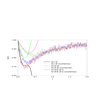
Figure 1: The form factor of a scatterer at a typical position, for some diffraction constants, thin lines, compared to the analytical result (11), heavy lines.

Agreement with (11) is found for short times, as is expected.

For a scatterer at the center only levels with wave functions that are symmetric with respect to the $X$ and $Y$ axes are perturbed by the scatterer. Since the value of these wave functions for all eigenvalues is the same ($\psi_{n}({\bf x}=0)=\frac{2}{\sqrt{\cal A}}$), the resulting equation is the same as for the Šeba billiard with periodic boundary conditions bogomolny01b . The form factor of the perturbed levels is related to the one of the full spectrum. The eigenvalues of the four different symmetry classes of the rectangle can be assumed to be uncorrelated, leading to

$$K_{full}(\tau)=\frac{3}{4}+\frac{1}{4}K_{per}(4\tau).$$ (12)

The form factor calculated from all levels and the scaled form factor obtained from the perturbed levels with the help of (12) are compared to the analytical result (9), for $D=-4i$, in Fig. 2.

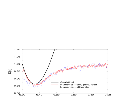
Figure 2: The form factor for the scatterer at the center (${\bf x}_{0}={\bf 0}$) compared to the scaled form factor calculated from perturbed levels (12) and the analytical result (9)

It is clear that (12) is valid. For very small times the full form factor deviates from its expected value since there are not enough orbits that contribute (the calculation is not semiclassical enough).

In order to study the effect of the angle dependence of the diffraction on the form factor it was calculated to the order $\tau^{2}$ for the diffraction constant (2). For a scatterer at a typical location the form factor is found to be long

$$K(\tau)=1-\frac{1}{4}|C|^{2}\tau+\frac{9}{128}|C|^{4}\tau^{2}+...~{}~{}~{}.$$ (13)

This form factor is similar to (11). Since $C$ of (3) satisfies the optical theorem (10), this form factor can also be obtained from an angle independent potential, with the diffraction constant $C$. If the scatterer is at the center long

$$K(\tau)=1-\frac{1}{4}|C|^{2}\tau+\frac{1}{8}|C|^{4}C^{\prime}\tau^{2}+....$$ (14)

with $C^{\prime}\equiv 1-2k^{2}a^{2}M_{0}$, where $M_{0}$ is related to integrals over the potential (1). It resembles the form factor (9) that was obtained for angle independent scattering. The modification is of the order $k^{2}a^{2}$ and typically cannot change the sign of the expansion coefficients.

The condition for the applicability of the approximations used in this letter is $a\ll\lambda\ll a_{x},~{}a_{y}$, where $\lambda$ is the wavelength of the particles . Up to corrections of order $(ka)^{3}$, the form factor (13) reduces to (11) in the order $\tau^{2}$. Therefore the angle dependence plays no role up to this order. If the scatterer is at the center the situation is somewhat different as can be seen comparing (14) with (9). There is a correction $C^{\prime}$ resulting of the angular dependence of $D(\theta^{\prime},\theta)$ given by (2). It is a consequence of the increased number of length degeneracies of the diffracting orbits when the scatterer is at the center. Since the form factor (13) describes essentially angle independent scattering the limit $a\rightarrow 0$ describes correctly the physics of the regime $a<\lambda$. This is so although the classical dynamics (in the long time limit) are expected to be chaotic in nearly all of phase space and similar to the ones of the Sinai billiard. This robustness improves the chances for the experimental realization of the results of the present work. For $a\gg\lambda$, semiclassical theory works and the system should behave as a Sinai billiard, with level statistics given by Random Matrix Theory (RMT) bohigas84 ; berry85 (with deviations, see sieber93 ).

The spectral statistics found in the present work differ from the ones of the known universality classes. It is characterized by the form factor of the type presented in Figs. 1 and 2. This form factor is equal to 1 at $\tau=0$, resulting of the fact that for small $\tau$ the number of classical orbits that are scattered is small. The contribution that is first order in $\tau$ originates from the combinations of forward diffracting orbits and periodic orbits. These always have the same lengths leading to the contribution $\Im D\tau$. By the optical theorem (10) it is always negative. For $\tau\gg 1$ the form factor approaches unity because of the discreteness of the spectrum berry85 . This general description should hold for other integrable systems, that are perturbed similarly.

- (1) Haake F., Quantum Signatures of Chaos, (Springer, New York, 1991).
- (2) Proceedings of the 1989 Les-Houches Summer School on “Chaos and Quantum Physics”, Giannoni M. J., Voros A. and Zinn-Justin, eds., (Elsevier, Amsterdam, 1991).
- (3) Bohigas O., Giannoni M. J. and Schmit C., Phys. Rev. Lett., 52, 1 (1984).
- (4) Berry M. V. and Tabor M., Proc. R. Soc. Lond., 356, 375 (1977).
- (5) Berry M. V., Proc. R. Soc. Lond., 400, 229 (1985).
- (6) Andreev A. V. and Altshuler B. L., Phys. Rev. Lett., 75, 902 (1995); Agam O., Altshuler B. L. and Andreev A. V., Phys. Rev. Lett., 75, 4389 (1995); Bogomolny E. B. and Keating J. P., Phys. Rev. Lett., 77, 1472 (1996).
- (7) Berry M. V. and Robnik M., J. Phys. A: Math. Gen., 17, 2413 (1984).
- (8) Izrailev F. M., Phys. Rep., 196, 299 (1990).
- (9) Šeba P., Phys. Rev. Lett., 64, 1855 (1990); Shigehara T., Phys. Rev. E, 50, 4357 (1994).
- (10) Bogomolny E., Gerland U. and Schmit C., Phys. Rev. E, 59, R1315 (1999); Bogomolny E., Giraud O. and Schmit C., Commun. Math. Phys., 222, 327 (2001); Rahav S. and Fishman S., Found. Phys., 31, 115 (2001); Narevich R., Prange R. E. and Zaitsev O., Physica E, 9, 578 (2001).
- (11) Bogomolny E., Gerland U. and Schmit C., Phys. Rev. E, 63, 036206 (2001).
- (12) Rahav S. and Fishman S., “Spectral statistics of rectangular billiards with localized perturbations”, to be published.
- (13) Bogomolny E. and Giraud O., “ Semi-classical calculations of the two-point correlation form factor for diffractive systems”, preprint, nlin.CD/0110006.
- (14) Marcus C. M., Rimberg A. J., Westervelt R. M., Hopkins P. F. and Gossard A. C., Phys. Rev. Lett., 69, 506 (1992); Chang A. M., Chaos, Solitons & Fractals, 8, 1281 (1997).
- (15) Stöckmann H. -J. and Stein J., Phys. Rev. Lett., 64, 2215 (1990); Sridhar S., Phys. Rev. Lett., 67, 785 (1991); Richter A., Found. Phys., 31, 327 (2001).
- (16) Friedman N., Kaplan A., Carasso D. and Davidson N., Phys. Rev. Lett., 86, 1518 (2001); Milner V., Hanssen J. L., Campbell W.C. and Raizen M. G., Phys. Rev. Lett., 86, 1514 (2001).
- (17) Gutzwiller M. C., J. Math. Phys, 8, 1979 (1967), 10, 1004 (1969), 11, 1791 (1970), 12, 343 (1971).
- (18) Gutzwiller M. C., Chaos in classical and quantum mechanics, (Springer, New York, 1990).
- (19) Berry M. V. and Tabor M., Proc. R. Soc. Lond., 349, 101 (1976); Berry M. V. and Tabor M., J. Phys. A: Math. Gen., 10, 371 (1977).
- (20) Keller J. B., J. Opt. Soc. Am., 52, 116 (1962).
- (21) Berkolaiko G., Bogomolny E. and Keating J. P., J. Phys. A: Math. Gen., 34, 335 (2001).
- (22) Sieber M., J. Phys. A: Math. Gen., 32, 7679 (1999), 33, 6263 (2000); Bogomolny E., Leboeuf P. and Schmit C., Phys. Rev. Lett., 85, 2486 (2000).
- (23) Bogomolny E., Nonlinearity, 13, 947 (2000).
- (24) Noyce H. P., Phys. Rev. Lett., 15, 538 (1965); Averbuch P. G., J. Phys. A: Math. Gen., 19, 2325 (1986).
- (25) Sieber M., Smilansky U., Creagh S. C. and Littlejohn R. G., J. Phys. A: Math. Gen., 26, 6217 (1993).