Abstract
We apply our recent formalism establishing new connections between the geometry of moving space curves and soliton equations, to the nonlinear Schrödinger equation (NLS). We show that any given solution of the NLS gets associated with three distinct space curve evolutions. The tangent vector of the first of these curves, the binormal vector of the second and the normal vector of the third, are shown to satisfy the integrable Landau-Lifshitz (LL) equation ${\bf S}_{u}={\bf S}\times{\bf S}_{ss}$, (${\bf S}^{2}=1$). These connections enable us to find the three surfaces swept out by the moving curves associated with the NLS. As an example, surfaces corresponding to a stationary envelope soliton solution of the NLS are obtained.

1 Introduction

A procedure to associate a completely integrable equation[1] supporting soliton solutions with the evolution equation of a moving space curve was found some time ago by Lamb [2]. Recently, we showed [3] that there are two other distinct ways of making such a connection. Thus three different space curve evolutions get associated with a given solution of the integrable equation. As an illustrative example, we considered the nonlinear Schrödinger equation (NLS) and demonstrated that the three associated moving curves had distinct curvature and torsion functions. We also obtained the curve parameters for a one-soliton solution of the NLS. However, as is well known[4], the explicit construction of an evolving space curve or swept-out surface, using the corresponding expressions for the curvature and torsion is a nontrivial task in general. For an integrable nonlinear partial differential equation, a method proposed by Sym [5] shows that using its Lax pair, a certain surface that gets associated with a given solution can be constructed, and this has been applied [6] to the NLS. In this paper, we use a different approach which obtains two more surfaces (or moving curves), in addition to the above surface. For the NLS, we first use the expressions[3] for the associated curve parameters to show that the three space curve evolutions all map to the integrable Landau-Lifshitz (LL) equation[7] for the time evolution of a spin vector ${\bf S}$ of a continuous one-dimensional Heisenberg ferromagnet. In other words, the tangent vector of the first moving curve, the binormal vector of the second, and the normal vector of the third, are shown to satisfy the LL equation. The first of these results is essentially the converse of the important mapping from the LL equation to the NLS which Lakshmanan[8] had obtained, by identifying S with the tangent vector. Exploiting the above connections enables us to explicitly construct the three swept-out surfaces. Surfaces associated with a stationary envelope soliton of the NLS are presented.

2 New connections between moving curves and soliton equations

A moving space curve embedded in three dimensions may be described[9] using the following two sets of Frenet-Serret equations[4] for the orthonormal triad of unit vectors made up of the tangent ${\bf t}$, normal ${\bf n}$ and the binormal ${\bf b}$:

$${\bf t}_{s}\ =\ K{\bf n}\ ;\ {\bf n}_{s}\ =\ -K{\bf t}\ +\ \tau{\bf b}\ ;\ {\bf b}_{s}\ =\ -\tau{\bf n}.$$ (1)

$${\bf{t}}_{u}\,=g{\bf{n}}+h{\bf{b}}\ ;\ {\bf{n}}_{u}\,=-g{\bf{t}}+\tau_{0}{\bf{b}}\ ;\ {\bf{b}}_{u}\,=\,-h{\bf{t}}-\tau_{0}{\bf{n}}.$$ (2)

Here, $s$ and $u$ denote the arclength and time respectively. The parameters $K$ and $\tau$ represent the curvature and torsion of the space curve. The parameters $g,h$ and $\tau_{0}$ are, at this stage, general parameters which determine the time evolution of the curve. All the parameters are functions of both $s$ and $u$. The subscripts $s$ and $u$ stand for partial derivatives. On requiring the compatibility conditions

$${\bf t}_{su}\ =\ {\bf t}_{us}\ ;\ {\bf n}_{su}\ =\ {\bf n}_{us}\quad;\quad{\bf b}_{su}\ =\ {\bf b}_{us},$$ (3)

a short calculation using Eqs. (1) and (2) leads to

$$K_{u}=(g_{s}-\tau h);~{}~{}\tau_{u}=(\tau_{0})_{s}+Kh;~{}~{}h_{s}=(K\tau_{0}-\tau g).$$ (4)

Formulation I: We shall refer to Lamb’s procedure [2] for associating moving space curves with soliton equations as ”formulation I”, to distinguish it from two others to follow. We remark that although Eq.(2) was not introduced by Lamb, his formulation implied them. As we shall see, its explicit introduction [9] proves very convenient in unraveling the geometry of the associated soliton equation. This formulation was motivated by Hasimoto’s earlier work [10], which had established a connection between the local induction equation for a vortex filament in a fluid [11] and the NLS. Here, one proceeds by defining a complex vector ${\bf N}=({\bf n}+i{\bf b})~{}~{}{\rm exp}[i\int\tau~{}ds]$ and the Hasimoto function

$$\psi(s,u)=K\exp{[i\int\tau~{}ds]}.$$ (5)

By writing ${\bf N}_{s},{\bf t}_{s},{\bf N}_{u}$ and ${\bf t}_{u}$ in terms of ${\bf t}$ and ${\bf N}$, imposing the compatibility condition ${\bf N}_{su}\ =\ {\bf N}_{us}$, and equating the coefficients of t and N in it, one obtains

$$\psi_{u}+\gamma_{1s}+(1/2)[\int~{}(\gamma_{1}\psi^{*}-\gamma_{1}^{*}\psi)~{}~{}ds]~{}\psi=0.$$ (6)

where

$$\gamma_{1}=-(g+ih)~{}~{}{\rm exp}[i\int\tau~{}ds]$$ (7)

The key step in Lamb’s work is that an appropriate choice of $\gamma_{1}$ as a function of $\psi$ and its derivatives can yield a known integrable equation for $\psi$. Comparing a solution of this equation with the Hasimoto function (5) yields the curvature $K$ and torsion $\tau$ of the moving space curve. Next, using the above mentioned specific choice of $\gamma_{1}$ in Eq. (7) yields the curve evolution parameters $g$ and $h$ as some specific functions of $K$, $\tau$ and their derivatives. Knowing these, $\tau_{0}$ can also be found from the third equality in Eq. (4). Thus a set of parameters $K$, $\tau$, $g$, $h$ and $\tau_{0}$ that correspond to a given solution of the integrable equation has been found. In other words, associated with this solution, there exists a certain moving space curve determined using Lamb’s procedure.

This raises the following question: Is this the only possible curve evolution that one can associate with an integrable equation, or are there others? We showed recently [3] that there are two other ways of making the association, which we call formulations II and III respectively, which lead to two other curve evolutions.
Formulation (II): Here, we combine the first two equations in Eqs.(1) to show that a complex vector ${\bf M}=({\bf n}-i{\bf t}){\rm exp}[i\int K~{}ds]$ and a complex function

$$\Phi(s,u)=\tau\exp{[i\int K~{}ds]},$$ (8)

appear in a natural fashion. By writing ${\bf M}_{s},{\bf b}_{s},{\bf M}_{u}$ and ${\bf b}_{u}$ in terms of ${\bf M}$ and ${\bf b}$, setting ${\bf M}_{su}\ =\ {\bf M}_{us}$, and equating the coefficients of b and M, respectively, we get

$$\Phi_{u}+\gamma_{2s}+(1/2)[\int~{}(\gamma_{2}\Phi^{*}-\gamma_{2}^{*}\Phi)~{}~{}ds]~{}\Phi=0.$$ (9)

where

$$\gamma_{2}=-(\tau_{0}-ih)~{}~{}{\rm exp}[i\int K~{}ds],$$ (10)

The subscript $2$ is used on $\gamma$ to indicate formulation (II).
Formulation (III): Here, we combine the first and third equations of (1), leading to the appearance of a complex vector ${\bf P}=({\bf t}-i{\bf b})$, and a complex function $\chi$ given by[12]

$$\chi(s,u)=(K+i\tau).$$ (11)

Next, writing ${\bf P}_{s},{\bf n}_{s},{\bf P}_{u}$ and ${\bf n}_{u}$ in terms of ${\bf P}$ and ${\bf n}$, imposing the compatibility condition ${\bf P}_{su}\ =\ {\bf P}_{us}$, and equating the coefficients of n and P, respectively, we get

$$\chi_{u}+\gamma_{3s}+(1/2)[\int~{}(\gamma_{3}\chi^{*}-\gamma_{3}^{*}\chi)~{}~{}ds]~{}\chi=0.$$ (12)

where

$$\gamma_{3}=-(g+i\tau_{0}).$$ (13)

Here, the subscript $3$ corresponds to formulation (III). Since Eq. (9) and Eq. (12) have the same form as Lamb’s equation (6), it is clear that for a suitable choice (see discussion following Eq. (7)) of $\gamma_{2}$ as a function of $\Phi$ and its derivatives, and of $\gamma_{3}$ as a function of $\chi$ and its derivatives, these equations can become known integrable equations for $\Phi$ and $\chi$ respectively.

Collecting our results, we see from Eqs. (5), (8) and (11) that the complex functions $\psi$, $\Phi$ and $\chi$ that satisfy the integrable equations in the three formulations are different functions of $K$ and $\tau$. Further, we see from Eqs. (7), (10) and (13) that the complex quantities $\gamma_{1}$, $\gamma_{2}$ and $\gamma_{3}$ that arise in these formulations also involve different combinations of the curve evolution parameters $g,h$ and $\tau_{0}$. Thus it is clear that these formulations indeed describe three distinct classes of curve motion that can be associated with a given integrable equation. (Our analysis suggests that this association may extend to some partially integrable equations as well.) Next, we apply these results to the NLS.

3 Application to the NLS

From our discussion given in the last section, it is easy to verify that in the three formulations, the respective choices

$$\gamma_{1}=-i\psi_{s};~{}~{}\gamma_{2}=-i\Phi_{s};~{}~{}\gamma_{3}=-i\chi_{s},$$ (14)

when used in Eqs. (6), (9) and (12), lead to the NLS

$$iq_{u}+q_{ss}+\frac{1}{2}|q|^{2}q=0,$$ (15)

with $q$ identified with the complex functions $\psi,\Phi$ and $\chi$ respectively. Now, a general solution of Eq. (15) is of the form $q=\rho\exp[i\theta]$. Equating this with the complex functions defined in Eqs.(5), (8) and (11) yields the curvature and the torsion of the space curves that correspond to that solution of the NLS to be ${\bf(I)}~{}\kappa_{1}=\rho,~{}~{}\tau_{1}={\theta}_{s},~{}~{}{\bf(II)}~{}\kappa_{2}={\theta}_{s},~{}~{}\tau_{2}=\rho$ and ${\bf(III)}~{}\kappa_{3}=\rho\cos\theta,~{}~{}\tau_{3}=\rho\sin\theta$. Thus clearly, three distinct space curves get associated with the NLS. However, even if $K$ and $\tau$ are known, to solve the Frenet-Serret equations (1) to find the tangent t of the curve, (in order to construct from it, the corresponding position vector ${\bf r}(s,u)=\int{\bf t}~{}~{}ds$ that describes the moving curve) is usually very cumbersome in general. In the present context, we shall show that a certain connection of the underlying curve evolutions of the NLS with the integrable LL equation via three distinct mappings enables us to construct these curves.

To proceed, first we equate the expressions for $\gamma_{1}$, $\gamma_{2}$ and $\gamma_{3}$ given in Eq. (14) with those given in Eqs. (7), (10) and (13) and obtain the following curve evolution parameters $g,h$ and $\tau_{0}$ in the three cases:
${\bf(I)}~{}~{}g_{1}=-\kappa_{1}\tau_{1};~{}~{}h_{1}=\kappa_{1s};~{}~{}\tau_{01}=(\kappa_{1ss}/\kappa_{1})-\tau_{1}^{2},\\ {\bf(II)}~{}~{}g_{2}=(\tau_{2ss}/\tau_{2})-\kappa_{2}^{2};~{}~{}h_{2}=-\tau_{2s};~{}~{}\tau_{02}=-\kappa_{2}\tau_{2},\\ {\bf(III)}~{}~{}g_{3}=-\tau_{3s};~{}~{}~{}h_{3}=(1/2)(\kappa_{3}^{2}+\tau_{3}^{2});~{}~{}\tau_{03}=\kappa_{3s}$.
Next, substituting these expressions for each of the formulations appropriately in Eq. (2), and using Eq. (1), a short calculation [3] shows that the LL equation[7]

$${\bf S}_{u}={\bf S}\times{\bf S}_{ss};~{}~{}~{}{\bf S}^{2}=1$$ (16)

is obtained in every case, i.e., for the tangent ${\bf t}_{1}$ of the moving space curve in the first formulation, for the binormal ${\bf b}_{2}$ in the second, and by the normal ${\bf n}_{3}$ in the third. Of the above, the first is just the converse of Lakshmanan’s mapping[8] where, starting with the LL equation (16), and identifying ${\bf S}$ with the tangent to a moving curve, it becomes possible to obtain the NLS for $\psi$. The other two clearly represent new geometries connected with the NLS. Furthermore, the converses of these two also hold good, i.e., starting with (16) and identifying ${\bf S}$ with ${\bf b}$ and ${\bf n}$ successively, we can show that the NLS for $\Phi$ and $\chi$ are obtained, respectively. These are the two analogs of Lakshmanan’s mapping. Next, we exploit these connections with Eq. (16) to find the moving space curves associated with the NLS.

The LL equation (16) has been shown to be completely integrable [13] and gauge equivalent[14] to the NLS. Its exact solutions can be found [13, 15]. We now show how ${\bf r}_{1}$, ${\bf r}_{2}$ and ${\bf r}_{3}$, the position vectors generating the three moving curves underlying the NLS, can be found in terms of an exact solution ${\bf S}$ of Eq. (16).

(I) Let ${\bf t}_{1}$ be the tangent to a certain moving curve created by a position vector ${\bf r}_{1}(s,u)$. Thus we set ${\bf t}_{1}={\bf r}_{1s}={\bf S}$, a solution of the LL equation. Now, the corresponding triad $({\bf t}_{1},{\bf n}_{1},{\bf b}_{1})$ of this curve satisfies the Frenet-Serret equations (1) with curvature $\kappa_{1}$ and torsion $\tau_{1}$. In terms of ${\bf t}_{1}$ (and hence ${\bf S}$), these are given by the usual expressions

$$\kappa_{1}=|{\bf t}_{1s}|=|{\bf S}_{s}|;~{}~{}\tau_{1}=\frac{{\bf t}_{1}.({\bf t}_{1s}\times{\bf t}_{1ss})}{{\bf t}^{2}_{1s}}=\frac{{\bf S}.({\bf S}_{s}\times{\bf S}_{ss})}{{\bf S}^{2}_{s}}$$ (17)

Thus the underlying moving curve ${\bf r}_{1}(s,u)$ in this formulation is simply given in terms of the solution ${\bf S}$ by

$${\bf r}_{1}(s,u)=\int{{\bf t}_{1}~{}ds}=\int{{\bf S}(s,u)~{}ds}$$ (18)

The above expression for ${\bf r}_{1}$ is the surface that one obtains using Sym’s[5] method.
(II) Let the binormal of some moving curve ${\bf r}_{2}(s,u)$ be denoted by ${\bf b}_{2}$. For this case, ${\bf b}_{2}={\bf S}$. Here, the tangent ${\bf t}_{2}={\bf r}_{2s}$. The triad $({\bf t}_{2},{\bf n}_{2},{\bf b}_{2})$ satisfies Eq. (1) with curvature $\kappa_{2}={\bf b}_{2}.({\bf b}_{2s}\times{\bf b}_{2ss})/|{\bf b}_{2s}|^{2}=\tau_{1}$ and torsion $\tau_{2}=\kappa_{1}$. (See Eq.(17)). Using ${\bf t}_{2}={\bf n}_{2}\times{\bf b}_{2}=-{\bf b}_{2}\times{\bf b}_{2s}/|{\bf b}_{2s}|=-{\bf S}\times{\bf S}_{s}/|{\bf S}_{s}|$, the position vector ${\bf r}_{2}(s,u)$ generating the second moving curve is found to be

$${\bf r}_{2}(s,u)=\int{{\bf t}_{2}~{}ds}=-\int{{\bf S}\times\frac{{\bf S}_{s}}{|{\bf S}_{s}|}~{}ds}$$ (19)

(III) Finally, let the normal of yet another moving curve ${\bf r}_{3}(s,u)$ be denoted by ${\bf n}_{3}$. So we have ${\bf n}_{3}={\bf S}$. The tangent of this curve is ${\bf t}_{3}={\bf r}_{3s}$, and the triad $({\bf t}_{3},{\bf n}_{3},{\bf b}_{3})$ satisfies Eq. (1) with curvature $\kappa_{3}$ and torsion $\tau_{3}$. Here, clearly, we need the expressions for ${\bf t}_{3}$ in terms of ${\bf n}_{3}$ and its derivatives. From Eq. (1) for this case,

$$(\kappa_{3}^{2}+\tau_{3}^{2}){\bf t}_{3}=\tau_{3}({\bf n}_{3}\times{\bf n}_{3s})-\kappa_{3}{\bf n}_{3s}$$ (20)

Next we find $\kappa_{3}$ and $\tau_{3}$ interms of ${\bf n}_{3}$ by showing that $({\bf n}_{3s})^{2}=(\kappa_{3}^{2}+\tau_{3}^{2})=\kappa_{1}^{2}$ and ${\bf n}_{3}.({\bf n}_{3s}\times{\bf n}_{3ss})/|{\bf n}_{3s}|^{2}=\tau_{1}=\frac{d}{ds}(\tan^{-1}(\tau_{3}/\kappa_{3}))$. Using $|{\bf n}_{3s}|=\kappa_{1}$, a short calculation yields $\kappa_{3}=\kappa_{1}\cos\eta_{1}$ and $\tau_{3}=\kappa_{1}~{}~{}\sin\eta_{1}$, where $\eta_{1}=[\int\tau_{1}~{}~{}ds~{}~{}+~{}~{}c_{1}(u)]$. Here, $c_{1}(u)$ is a function of time $u$ , which can be found in terms of $\kappa_{1}$ and $\tau_{1}$ using the appropriate Eqs. (4) for $\kappa_{3u}$ and $\tau_{3u}$. These details will be given elsewhere. Substituting the above values for $\kappa_{3}$ and $\tau_{3}$ into Eq. (20), and setting ${\bf n}_{3}={\bf S}$, the position vector ${\bf r}_{3}(s,u)$ creating the third moving space curve can be found to be

$${\bf r}_{3}(s,u)=\int{\bf t}_{3}~{}ds=\int\frac{[({\bf S}\times{\bf S}_{s})\sin\eta_{1}-{\bf S}_{s}~{}~{}\cos\eta_{1}])}{\kappa_{1}}~{}ds$$ (21)

4 Example: Soliton geometries

Defining three orthogonal unit vectors ${\bf\hat{e}}_{1}=\Big{\{}1,0,0\Big{\}},~{}{\bf\hat{e}}_{2}=\Big{\{}0,\cos\eta,\sin\eta\Big{\}},~{}{\bf\hat{e}}_{3}=\Big{\{}0,-\sin\eta,\cos\eta\Big{\}}$, a soliton solution of the LL equation (16) is given by

$${\bf S}(s,u)=(1-\mu\nu{\rm sech}^{2}(\nu\xi)){\bf\hat{e}}_{1}{}$$ (22)

$${}+\mu\nu{\rm sech}(\nu\xi)\tanh(\nu\xi){\bf\hat{e}}_{2}-\mu\lambda{\rm sech}(\nu\xi){\bf\hat{e}}_{3}$$

where $\xi=(s-2\lambda u),\eta=(\lambda s+(\nu^{2}-\lambda^{2})u)$, and $\mu=2\nu/(\nu^{2}+\lambda^{2})$. Here, $\nu$ and $\lambda$ are arbitrary constants. Using Eq.(22) and our results of the previous section, the three moving curves that correspond to the soliton solution $q=~{}\rho~{}\exp{i\theta}=~{}2\nu{\rm sech}(\nu\xi)~{}\exp{i\eta}$ of the NLS (Eq. (15)) are found by substituting Eq. (22) in Eqs. (18), (19) and (21), respectively. For the sake of illustration, let us consider the special case $\lambda=0$, which corresponds to the velocity of the envelope of the NLS soliton being zero. We obtain the following three swept-out surfaces:

$${\bf(I)}~{}~{}{\bf r}_{1}=[s-(2/\nu)\rm tanh\nu s,(-2/\nu)\rm sech\nu s~{}\cos\nu^{2}u,{}$$

$${}(-2/\nu)\rm sech\nu s~{}\sin\nu^{2}u]$$ (23)

Note that $\kappa_{1}=2\nu{\rm sech}(\nu s)$ and $\tau_{1}=0.$ This surface is given in Fig. (1).

$${\bf(II)}~{}~{}{\bf r}_{2}=s~{}~{}~{}[~{}~{}0,~{}~{}~{}\sin\nu^{2}u,~{}~{}~{}-\rm\cos\nu^{2}u~{}~{}]$$ (24)

Here, $\kappa_{2}=0$ and $\tau_{2}=2\nu{\rm sech}(\nu s)$. For the sake of completeness, we display this planar surface in Fig. (2).

$${\bf(III)}~{}~{}{\bf r}_{3}=[(2/\nu){\rm sech}\nu s~{}\cos(\nu^{2}u),~{}(s-(2/\nu)\tanh\nu s$$

$$\cos^{2}(\nu^{2}u)),-(2/\nu)\tanh\nu s\cos(\nu^{2}u)\sin(\nu^{2}u)]$$ (25)

Here, $\kappa_{3}=2\nu{\rm sech}\nu s~{}~{}\cos\nu^{2}u$ and $\tau_{3}=2\nu{\rm sech}\nu s~{}~{}\sin\nu^{2}u.$ This surface is given in Fig. (3).

For the case $\lambda\neq 0$, the envelope of the NLS soliton moves. Geometrically, this motion can be shown to correspond to the ”twisting out” of the surface in Fig. (1), around its symmetry axis, and ”stacking up” of more such surfaces in a helical fashion along this axis. This leads to corresponding changes in Figs. (2) and (3) as well. The details of this will be presented elsewhere.

Before we conclude, we mention that the geometry underlying the NLS can also be studied by working with the complex conjugates of the complex vectors and functions that we used in the three formulations. These can be shown to lead to a mapping to the LL equation for ${\bf-t},{\bf-n}$ and ${\bf-b}$ respectively. It can be verified that these merely yield surfaces which are created by the negative of the position vectors ${\bf r}_{i},i=1,2,3$, which we found in Section 3, so that essentially no new surfaces result from these. Finally, while in the first formulation, it can be easily verified that the curve velocity ${\bf r}_{1u}$ satisfies the local induction equation[11] ${\bf r}_{1u}~{}=~{}\kappa_{1}{\bf b}_{1}$, the velocities ${\bf r}_{2u}$ and ${\bf r}_{3u}$ appearing in the other two formulations can be shown to satisfy more complicated equations. These general results on curve kinematics and their ramifications are reported in [16].

Figure Captions:

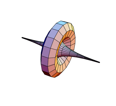
Figure 1: Surface swept-out by the moving space curve ${\bf r}_{1}(s,u)$ (Eq. (S0.Ex2)) for $\nu=1$ and $0\leq u\leq 6.3$.

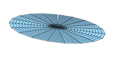
Figure 2: Surface swept-out by the moving space curve ${\bf r}_{2}(s,u)$ (Eq. (24)) for $\nu=0.5$ and $0\leq u\leq 25$.

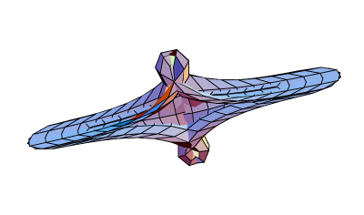
Figure 3: Surface swept-out by the moving space curve ${\bf r}_{3}(s,u)$ (Eq. (S0.Ex3)) for $\nu=0.5$ and $0\leq u\leq 25$.

References

- [1] See, for instance, M.J. Ablowitz and H. Segur, Solitons and the Inverse Scattering Transform, ( SIAM, Philadelphia,1981).
- [2] G.L. Lamb, J. Math. Phys. 18, 1654 (1977) .
- [3] S. Murugesh and Radha Balakrishnan, Phys. Lett. A 290, 81 (2001); nlin. PS/0104066.
- [4] See, for instance, D.J.Struik, Lectures on Classical Differential Geometry (Addison-Wesley, Reading, MA 1961).
- [5] A.Sym, Lett. Nuovo Cimento 22, 420 (1978) ;
- [6] D. Levi, A. Sym and S. Wojciechowski, Phys. Lett. A 94, 408 (1983).
- [7] L.D. Landau and E. M. Lifshitz, Phys. Z Sowjet 8, 153 (1935).
- [8] M. Lakshmanan, Phys. Lett. A 61, 53 (1977).
- [9] Radha Balakrishnan, A. R. Bishop, R. Dandoloff, Phys. Rev. B 47, 3108 (1993); Phys. Rev. Lett. 64, 2107 (1990); Radha Balakrishnan and R. Blumenfeld, J. Math. Phys. 38, 5878 (1997).
- [10] H. Hasimoto, J. Fluid. Mech. 51, 477 (1972).
- [11] L. S. Da Rios, Rend. Circ. Mat. Palermo 22, 117 (1906); For history, see R. L. Ricca, Nature 352, 561 (1991).
- [12] These definitions for and , which are the complex conjugates of those used in our Ref. [3], prove to be more convenient for our purpose.
- [13] L.A. Takhtajan, Phys. Lett. A 64, 235 (1977).
- [14] V. E. Zakharov and L. A. Takhtajan, Theor. Math. Phys. 38, 26 (1979).
- [15] J. Tjon and J. Wright, Phys. Rev. B 15, 3470 (1977).
- [16] Radha Balakrishnan and S. Murugesh, Theor. Math. Phys. (submitted); nlin. SI/0111048