Sensitivity to perturbations in a quantum chaotic billiard

Abstract

The Loschmidt echo (LE) measures the ability of a system to return to the initial state after a forward quantum evolution followed by a backward perturbed one. It has been conjectured that the echo of a classically chaotic system decays exponentially, with a decay rate given by the minimum between the width $\Gamma$ of the local density of states and the Lyapunov exponent. As the perturbation strength is increased one obtains a cross-over between both regimes. These predictions are based on situations where the Fermi Golden Rule (FGR) is valid. By considering a paradigmatic fully chaotic system, the Bunimovich stadium billiard, with a perturbation in a regime for which the FGR manifestly does not work, we find a cross over from $\Gamma$ to Lyapunov decay. We find that, challenging the analytic interpretation, these conjetures are valid even beyond the expected range.

Hypersensitivity to initial conditions is the key ingredient of classical chaos. In quantum mechanics, its absence led to the study of other features that could be associated with the chaos of the corresponding classical system. Celebrated examples are the Gutzwiller trace formula for the quantum spectral density, the description of the spectral fluctuations by the random matrix theory and the relation of spectral correlations to transport [1, 2].

In an alternative point of view, Peres [3] suggested that quantum dynamics should distinguish regular and irregular classical dynamics if the time evolution of an initial state for slightly different Hamiltonians are compared. That is, the sensitivity of a quantum system should be searched not by changing the initial conditions but rather by perturbing the Hamiltonian. The natural quantity for this investigation is the ability of the system to return to the initial state $\left|\phi\right\rangle\,$ after being evolved with a Hamiltonian ${\cal H}_{0}$ for a period $t$ followed by an identical period of unitary evolution with $-{\cal H}_{1}=-({\cal H}_{0}+\Sigma).$ This defines the quantum Loschmidt echo (LE)

$$M(t)=|\left\langle\phi\right|\exp[{\rm i}{\cal H}_{1}t/\hbar]\exp[-{\rm i}{\cal H}_{0}t/\hbar]\left|\phi\right\rangle|^{2}.$$ (1)

The perturbation $\Sigma$ can represent the uncontrolled degrees of freedom of an environment. As in classical chaos, the LE is related to a ‘distance’ between a perturbed and an unperturbed evolution of the same initial state.

In recent years new hints were available due to the advances in Nuclear Magnetic Resonance. The LE was measured in a many-body system of interacting spins [4] in a range where it is known to have spectral signatures of chaos. A striking finding was that, when interaction with the environment and residual interactions are very weak, the decay of $M(t)$ becomes independent of the perturbation strength. In this situation, it depends on the dynamical scales of the systems, i.e. on ${\cal H}_{0}$. While the complexity of the experimental system did not allow for a derivation of the characteristic time for these specific system, Jalabert and Pastawski [5] studied the LE in a one-body classically chaotic Hamiltonian with a perturbation represented by a long range quenched disordered potential. They have showed analytically that $M(t)$ may decay exponentially with a rate given by the Lyapunov exponent of the classical system. As condition, the perturbation must be quantically strong to produce statistically unpredictable changes in the quantum phase but weak enough to leave the underlying classical dynamics undisturbed.

More recently, Jacquod, Silvestrov and Beenakker [6] predicted a cross-over from a perturbation dependent regime to the Lyapunov one. However, this prediction is based on the strong assumption that the perturbation lives in a FGR regime; i.e. the local density of states (LDOS) is a Breit-Wigner distribution whose width $\Gamma$ varies quadratically with the perturbation strength. In this situation, $M(t)$ for a wave packet and the survival probability of an unperturbed eigenstate have a decay rate given by $\Gamma.$ Both observables would describe the same physics if the correlation between states forming the wave packet could be neglected.

Our aim is to determine whether the perturbation independent Lyapunov regime and the cross-over from a $\Gamma$ decay are possible in a fully chaotic system with a clear semiclassical description where the presence of the perturbation is not described by the FGR. This occurs when there are strong correlations that could be related to classical structures which prevents a description in terms of a random matrix theory. This perturbation is then said to be non generic [7] and the LDOS can be very different from the Lorentzian analyzed in Ref. [6]. Our positive answer in such a case opens the question of a semiclassical interpretation for the weak perturbation regime.

We consider the paradigmatic disymmetrized Bunimovich stadium billiard [8]. It consists of a free particle inside a 2-dimensional planar region whose boundary ${\cal C}$ is shown in Fig.  1. The radius $r$ is taken equal to unity and the enclosed area is $1+\pi/4$. This system not only has a great experimental relevance [9, 10], but also it is fully chaotic one by oposition to the system considered in Ref.[6]. Besides, it can rule out the diffusive effect of disorder suspected to affect the behavior of $M(t)$ in a Lorentz gas[11]. The classical dynamics is completely defined once the boundary is given. On the other hand, to address the quantum mechanics, it is necessary to solve the Helmholtz equation, $\nabla^{2}\phi_{\mu}=k^{2}\phi_{\mu}$ with appropriate boundary conditions. $k_{\mu}$ is the wave number and by setting $\hbar=2m=1$, $k_{\mu}^{2}$ results the energy. The most commonly used boundary conditions are the Dirichlet (hard walls) and the Neumann (acoustics) conditions. However, we are interested in the possibility of perturbing the quantum system without breaking the orthogonal symmetry and leaving the classical motion undisturbed [2]. This is possible using more generalized boundary conditions:

$$\phi(q)\;+\;\xi\;g(q)\frac{\partial\phi}{\partial{\bf n}}(q)=0,$$ (2)

where $q$ is a coordinate along the boundary of the billiard (see Fig.  1), and ${\bf n}$ is the unit vector normal to the boundary. $g(q)$ is a real function and $\xi$ the parameter controlling the strength of the perturbation. Dirichlet boundary conditions are recovered when $\xi=0$ while Neumann conditions are satisfied in the limit $\xi\rightarrow\infty$. The eigenfunctions and eigenenergies for the case $\xi=0$ are readily obtained by using the scaling method[12].

In order to compute the LE in this system, a relation between the eigenvalues and eigenfunctions for different values of the parameter $\xi$ is needed. Based on a recently developed Hamiltonian expansion for deformed billiards [13], it is easy to show that the eigenvalues and eigenfunctions for different values of the parameter $\xi$ can be obtained from the Hamiltonian ${\cal H}_{0}+\Sigma(\xi)$ which is expressed in the basis of eigenstates at $\xi=0$ (from now on we will call $\phi_{\mu}$ to these eigenstates),

$$\Sigma_{\mu\nu}=\xi\times{\rm\Phi}_{\mu\nu}\;\oint_{{\cal C}}g(q)\;\frac{\partial\phi_{\mu}}{\partial{\bf n}}\frac{\partial\phi_{\nu}}{\partial{\bf n}}{\rm d}q.$$ (3)

The function $g(q)$ measures the strength of the change in the boundary condition along the contour. Within a perturbation theory it would represent the direction and strength of a distortion of the stadium [13]. Here we use

$\displaystyle g(q)=\left\{\begin{array}[]{ccc}\alpha&&0\leq q\leq 1,\\ (1+\alpha)\sin(q-1)+\alpha&&1<q\leq 1+\pi/2\end{array}\right.$

with $\alpha=-1/(2+\pi/2)$ that could be assimilated to a dilation along the horizontal axis and a contraction along the perpendicular one.  Notice that the integral above could be viewed as an inner product among the wave functions $\frac{\partial\phi_{\mu}}{\partial{\bf n}}$ defined over ${\cal C}$. This relation defines an effective Hilbert space in a window $\Delta k\approx$ Perimeter/Area [13]. The cut-off function ${\rm\Phi}_{\mu\nu}=\exp\left[-2\;(k_{\mu}^{2}-k_{\nu}^{2})^{2}/(k_{0}\Delta k)^{2}\right]$ restricts the effect of the perturbation to states in this energy shell of width $B\simeq k_{0}\Delta k$. It allows to deal with a basis of finite dimension with wave numbers around the mean value $k_{0}$ and restricting to a particular region $\Delta k$  of interest.

Figure  1 shows  the dependence of the energy levels on the perturbation. They exhibit many avoided crossings as $\xi$ is varied. While the energy levels show the typical behavior of a general system without constants of motion, we also recognize that some small avoided crossings are situated along parallel tilted lines. These energies correspond to the well known “bouncing ball” states which are highly localized in momentum. The selected perturbation does not modify substantially those states.

Since the LE is a classically motivated quantity, a Gaussian wave packet (with a mean value of momentum $k_{0}$ and velocity $v_{0}$) is a proper semiclassical selection for an initial condition. By evaluating its evolution in a system without perturbation ($\xi=0$) and other with perturbation strength $\xi$, we compute the LE (Eq. 1) as a function of time. At this point one must recognize that the choice of a semiclassical initial condition is very relevant in order to observe the ’Lyapunov’ regime [14, 6].

While a global exponential decay of $M(t)$ can be clearly identified in almost any individual initial condition, the fluctuations for a system with $k_{0}$ not too large can introduce error in the estimation of the rate. Hence, we have taken an average over $30$ initial states. Fig. (2) (a) and (b) show typical sets of curves of $M(t)$ for $k_{0}=50$ and $k_{0}=100$ respectively. It can be seen that after a transient, $M(t)$ decays exponentially, $\sim\exp[-t/\tau_{\phi}]$. For $\xi>\xi_{c}\simeq 4.5/k$   the decay rate $\tau_{\phi}$ becomes independent of the perturbation and $1/\tau_{\phi}\approx\lambda$ with $\lambda$ the Lyapunov exponent of the classical system [16] in accordance with the conjecture.   On the other hand, for large times $M(t)$ saturates to a finite value $M_{\infty}\approx 1/N$ with $N$ the effective dimension of the Hilbert space [3].  

According to Ref. [5] the chaos controlled decay appears provided that $\lambda>1/\widetilde{\tau}$ where $\widetilde{\ell}=v_{o}\widetilde{\tau}$ is the length over which the perturbation changes the quantum phase (mean free path) which, for a plane wave with wave number $k$ and velocity $v_{o}$. For a quenched disorder perturbation is evaluated from the FGR [5]

$$\frac{1}{\widetilde{\tau}_{k}}=\frac{2\pi}{\hbar}\lim_{\eta\rightarrow 0^{+}}\sum_{k^{\prime}}\left|\Sigma_{k^{\prime}k}\right|^{2}{\textstyle{\frac{1}{\pi}}}\frac{\eta/2}{(E_{k^{\prime}}-E_{k})^{2}+(\eta/2)^{2}}.$$ (4)

Ref. [6] realized that in the opposite regime of $\lambda<1/\widetilde{\tau},$   the LE  of an eigenstates $\phi_{\mu}$ of ${\cal H}_{0}$ is just a survival probability an must decay exponentially under the action of the perturbation,

$$|\left\langle\phi_{\mu}\right|\exp[{\rm i}\left({\cal H}_{0}{\cal+}\Sigma\right)t/\hbar]\left|\phi_{\mu}\right\rangle|^{2}\sim\exp[-t/\widetilde{\tau}_{\mu}],$$ (5)

given by Eq. 4 for$\,\,\,\hbar/B<t<\hbar/\Delta$ ($\Delta$ the mean level spacing) [17]. The appearance of this FGR behavior requires that a typical matrix element $U\simeq\left\langle\left|\Sigma_{\mu\nu}\left(\xi\right)\right|\right\rangle_{{\rm typ.}}$of the perturbation to be $U>\Delta.$ The Fourier transform of Eq. 5 is the LDOS which, although being discrete, would present a Lorentzian envelope [18] of width $\Gamma=1/\widetilde{\tau}$. In Ref. [6] it is conjectured that this decay can determine the LE decay with more general initial states. This is the regime controlled by the non-diagonal terms in the semiclassical expansion [5]. Once the non-diagonal terms have decayed, one expects the chaos controlled decay of the diagonal ones will survive. This gives a cross-over criterion for the decay rate of the LE of $1/\tau_{\phi}=\min[\Gamma,\lambda]$ as the perturbative parameter $\xi$ changes.

The LDOS is shown in Fig.  3 for three different perturbation strengths. In contrast to the case of Ref. [6] our distribution is not Lorentzian. This is related to the fact that the used perturbation (the function $g(q)$) does not connect all different regions of phase space; for instance, the bouncing ball states are practically undisturbed by $\Sigma$ determining the non-generic nature of the perturbation. In particular, we have evaluated the width $\Gamma,$ showing the spreading of the unperturbed eigenstates when expressed in terms of the new ones. The results show a linear dependence of $\Gamma$ on $\xi\,$ shown in Fig. 3; that is, we obtain $\Gamma\simeq 0.36\xi k^{2}$.  Moreover, taking into account that $\lambda\simeq 0.86k$, the critical value $\xi_{c}$ for the crossover from the $\Gamma$ regime to the Lyapunov one is expected at $\xi_{c}=2.4/k$ (remember that from Fig.  2 it results $\xi_{c}\approx 4.5/k$). Then, for our system, the criterium works with a $\Gamma$ given by the half width of the LDOS. This is shown in Fig.  4 where for perturbation strengths $\xi<4.5k^{-1}$, the LE. decays as $M(t)=\exp\left[-t/\tau_{\phi}\right]\,\,\,1/\tau_{\phi}=\Gamma/2$ for $\lambda>\Gamma/2$.

These results contrast with the FGR dependence of $1/\tau_{\phi}\propto\xi^{2}$ observed for weak perturbations. These are the Lorentz gas with a perturbed effective mass [11],  the kicked top perturbed by a perpendicular delayed kick[6] and general chaotic system perturbed by a quenched disorder[5] where random matrix theory describes[19] the $\Gamma$ decay. In this context, the linear dependence of $1/\widetilde{\tau}$ on $\xi$ may be considered as a further indicative that the physics of the LE decay can be very different from that described by Eq. 5 and that the result of Ref. [6] has more general validity than expected. In the non-perturbative regime, before the Lyapunov exponent takes over,the LE decays exponentially with a rate given by the perturbation dependent width of the LDOS. Another important feature is that $\xi_{c}\simeq 4.5/k\,\rightarrow 0$ when $k\rightarrow\infty.$ This confirms that in the classical limit Eq. (1) would decay with the Lyapunov regime regardless of the magnitude of $\Sigma$, recovering the chaotic hypersensitivity to perturbations.

In summary, by studying one of the most important models in quantum chaos, a fully chaotic billiard system, we have shown that, for a wide range of parameters, the Loschmidt echo decays exponentially with rate given by the Lyapunov exponent of the classical system. Moreover, we have discussed the onset of this Lyapunov regime requires that $\lambda>\Gamma/2.$ In the opposite situation, the presence of an exponential controlled by $\Gamma$ even in absence of a generic perturbation described by the FGR, demands further studies to fully interpret the detailed mechanism controlling this regime. We finally remark that the $M(t)$ would behave much differently for intrisically quantum initial conditions. For an eigenstate of ${\cal H}$ one finds a decay described by a FGR and it does not show a crossover into the Lyapunov decay [14]. In the other quantum extreme, an initial state generated from the long time evolution of a semiclassical wave packet[20], we find a perturbation dependent Gaussian decay [21]. These issues have begun to receive much attention [22] due to its strong connection with quantum computing stability, decoherence in waves, and quantum-classical transition. Furthermore, the dephasing time observed in transport experiments in mesoscopic devices shows a perturbation independent rate [9]. So far, there is no consensus about the physical phenomenon causing it. Since the time scale $\tau_{\phi}$ measured by the LE is a decoherence time and our methodology can obviously be adapted to treat the transport problem [2], our results open a rich field for exploration: the connection of both time scales.

We thank D. Cohen, R. Jalabert and M. Saraceno for very useful discussions and the support from SeCyT-UNC, CONICET, ANPCyT, ECOS-SeTCIP and Antorchas-Vitae. DAW received support from CONICET (Argentina) and AECI (Spain).

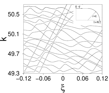
FIG. 1.: Spectrum of the desymmetrized stadium billiard with mixed boundary conditions controled by the parameter $\xi$ [Eq. (3)]. The wave numbers $k_{\mu}(\xi)$ run between 49.3 and 50.7. Inset: Schematic figure of the system. In solid line we show the boundary of the stadium billiard where the mixed boundary conditions are applied [Eq. (2)]. The coordinate $q$ on the boundary is also shown. Dashed lines correspond to the symmetries axis with Dirichlet boundary conditions.

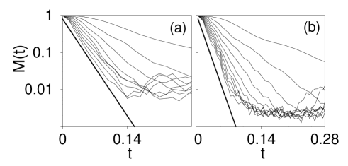
FIG. 2.: $M(t)$ for the desymmetrized stadium billiard perturbed by a change in the boundary conditions. The calculations is shown in two different energy regions. (a) Corresponds to the region around $k_{0}=50$. The value of $\xi$ is, from the top curve to bottom: 0.019, 0.038, 0.057, 0.075, 0.094, 0.11, 0.13, 0.15 and 0.17. (b) Corresponds to the region around $k_{0}=100$. The value of $\xi$ is, from the top curve to bottom: 0.0066, 0.0131, 0.020, 0.0262, 0.0327, 0.0393, 0.0458, 0.0524, 0.0589, 0.066, and 0.072. The thick lines corresponds to an exponential decay with decay rate $\tau_{\phi}=1/\lambda$.

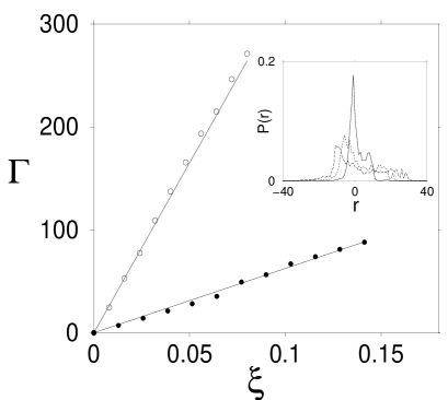
FIG. 3.: Width $\Gamma$ of the local density of states as a function of the perturbation strenght $\xi$ for $k_{0}=50$ (filled circles) and $k_{0}=100$ (circles). The solid lines are the best linear fit. Inset: Local density of states $P(r)$ for diferent perturbations in $k_{0}=50$ (r is measured in mean level spacing units).

FIG. 4.: $M(t)$ as a function of the rescaled time $\xi t$ for $k_{0}=50$ and $\xi=$ 0.019, 0.038, 0.057 and 0.075. The dotted line gives the decay $M(t)=\exp(-\Gamma t/2)$.

REFERENCES

- [1] H.–J. Stöckmann, Quantum Chaos: An Introduction (Cambridge U. Press, Cambridge, 1999).
- [2] A. Szafer and B. Altshuler, Phys. Rev. Lett. 70, 587 (1993).
- [3] A. Peres, Phys. Rev. A 304, 1610 (1984).
- [4] H. M. Pastawski, G. Usaj and P. R. Levstein, Chem. Phys. Lett. 261, 329 (1996); H. M. Pastawski, P. R. Levstein, G. Usaj, J. Raya and J. Hirschinger, Physica A 283, 166 (2000).
- [5] R. Jalabert and H. M. Pastawski , Phys. Rev. Lett. 86, 2490 (2001).
- [6] Ph. Jacquod, P. G. Silvestrov, C. W. J. Beenakker, Phys. Rev. E 64, 055203 (2001)
- [7] D. Cohen, A. Barnett and E.J. Heller, Phys. Rev. E 63, 46207 (2001).
- [8] L. A. Bunimovich, Funct. Anal. Appl. 8, 254 (1974).
- [9] A. G Huibers et al. Phys. Rev. Lett. 83, 5090 (1999)
- [10] M. Switkes, C. M. Marcus, K. Campman and A. C. Gossard, Science 283, 1905 (1999).
- [11] F. M. Cucchietti, H. M. Pastawski and D. A. Wisniacki, Phys. Rev. E in press, cond-mat/0102135.
- [12] E. Vergini and M. Saraceno, Phys. Rev. E 52, 2204 (1995).
- [13] D. A. Wisniacki and E. Vergini, Phys. Rev. E 59, 6579 (1999).
- [14] D. A. Wisniacki and D. Cohen, quant-ph/0111125.
- [15] D. Cohen and E.J. Heller, Phys. Rev. Lett 84, 2841 (2000).
- [16] Ch. Dellago and H. A. Posch, Phys. Rev. E 53, 2401 (1995).
- [17] F. M. Cucchietti, H. M. Pastawski, E. Medina and G Usaj, Anales AFA 10, 224 (1998).
- [18] Ph. Jacquod and D. L. Shepelyansky, Phys. Rev. Lett. 75, 3501 (1995)
- [19] F. M.Cucchietti et al., nlin.CD/0112015.
- [20] Z. P. Karkuszewski, C. Jarzynski, W. H. Zurek. quant-ph/0111002
- [21] F. M. Cucchietti, et al. (unpublished)
- [22] P. G. Silvestrov, H. Schömerus, and C. W. J. Beenakker, Phys. Rev. Lett. 86 5192 (2001); T. Prosen and M. Znidaric. nlin.CD/0111014; N. R. Cerruti and S. Tomsovic. Phys. Rev. Lett. 88 054103 (2002); T. Gorin and T. H. Seligman, quant-ph/0112030.