The role of diffusion in the chaotic advection of a passive scalar with finite lifetime

Abstract

We study the influence of diffusion on the scaling properties of the first order structure function, $S_{1}$, of a two-dimensional chaotically advected passive scalar with finite lifetime, i.e., with a decaying term in its evolution equation. We obtain an analytical expression for $S_{1}$ where the dependence on the diffusivity, the decaying coefficient and the stirring due to the chaotic flow is explicitly stated. We show that the presence of diffusion introduces a crossover length-scale, the diffusion scale ($L_{d}$), such that the scaling behaviour for the structure function is analytical for length-scales shorter than $L_{d}$, and shows a scaling exponent that depends on the decaying term and the mixing of the flow for larger scales. Therefore, the scaling exponents for scales larger than $L_{d}$ are not modified with respect to those calculated in the zero diffusion limit. Moreover, $L_{d}$ turns out to be independent of the decaying coeficient, being its value the same as for the passive scalar with infinite lifetime. Numerical results support our theoretical findings. Our analytical and numerical calculations rest upon the Feynmann-Kac representation of the advection-reaction-diffusion partial differential equation.

I Introduction

The subject of advection of (chemically or biologically) reacting substances is of major importance in fields ranging from combustion to water quality control (see for example [1]). One of the simplest models of reaction occurring in a flow is the decrease at a constant rate in the concentration of a substance. Radioactive or photochemical decay belong to this class of reactions. The spatial structure of the decaying chemical under chaotic fluid stirring has been described in recent works [2, 3] with emphasis on the microstructure formation by the stretching properties of the flow, at scales at which molecular diffusion can be neglected. The interpretation of real data, specially in laboratory experiments in which the diffusion scale may be explicitely resolved, requires however the consideration of diffusive processes which tend to homogeneize the structure at the smallest scales.

In this paper we investigate the role of the molecular diffusion in the scaling properties of the first order structure function, defined below (3) when $q=1$, for a passive scalar advected by a two-dimensional flow yielding Lagrangian chaos, and with finite lifetime. Thus, the passive scalar field (passive in the sense that there is no back influence on the hydrodynamics) $\phi({\bf x},t)$ evolves according to

$$\frac{\partial\phi({\bf r},t)}{\partial t}+{\bf v}({\bf r},t)\cdot\nabla\phi({\bf r},t)=\nu\nabla^{2}\phi({\bf r},t)-b\phi({\bf r},t)+S({\bf r}),$$ (1)

where $\nu$ is the diffusivity, $-b\phi$ represents the decaying and indicates that the passive scalar field decays with time at rate $b>0$, $S({\bf r})$ is a steady source of the passive scalar, and finally, ${\bf v}({\bf x},t)$ is the velocity of the flow. Here we assume that the velocity field is two-dimensional, incompressible, smooth, and nonturbulent. Chaotic advection in two dimensions is obtained generically if a time dependence (periodic, for e.g.) is included in ${\bf v}({\bf x},t)$ [4].

Eq. (1) can be considered as an approximation to more complex biological or chemical phenomena, like the dynamics of plankton populations in ocean currents [5, 6] and the advection of pollutants or chemical substances in the atmosphere [7], or as a description of simple procceses, like the relaxation of the sea surface temperature [8]. Moreover, in [9] it is argued that, in a determined scale range, the vorticity of a turbulent flow may evolve passively according to Eq. (1), indicating the high relevance of this equation in the studies of two-dimensional turbulence.

In the different case of a turbulent velocity field, the spatial propiertes, neglecting intermittency corrections, of a scalar field evolving through Eq. (1) were first written down by Corrsin [10]. The analytical expression for the power spectrum was obtained, among other situations, in the Batchelor’s regime, that is, between the smallest typical length scale of the velocity field and the characteristic length scale of diffusion ($L_{d}$), and from this, the scaling exponents and the diffusion length scale, $L_{d}$, were derived. The calculated form of the power spectrum $\Gamma(k)$ is

$$\Gamma(k)=Nk^{(2b/\lambda)-1}exp(-2\nu k^{2}/\lambda),$$ (2)

where $N$ is a constant and $\lambda$ is the absolute value of the most negative of the average stretching rates. However, no numerical test of this result, checking the influence of molecular diffusion on the crossover, has been reported. Moreover, the criticisms made by Kraichnan [11] to the crossover of the power spectrum calculated by Batchelor [12] for a passive scalar with infinite lifetime, $b=0$, as being too sensible to the intermittency, can also be applied here.

In this paper we study the case of a smooth (nonturbulent) chaotic flow, and instead of the power spectrum we calculate the first order structure function. In the absence of diffusion, the scaling exponents for the structure functions were calculated neglecting intermittency corrections [2], or including them for smooth chaotic flows [3, 13], and in [14] for the Kraichnan flow in the spatially smooth limit. The structure functions are important quantities than can yield information about the typical variation of the concentration field over a small distance $\delta x$. Thus, a structure function of order $q$ is defined as

$$S_{q}(\delta x)=<|\delta\phi|^{q}>=<|\phi({\bf x}+\delta x{\bf n})-\phi({\bf x})|^{q}>,$$ (3)

where $<>$ denotes spatial average, ${\bf n}$ is a unit vector in the chosen direction, and $q$ is a positive real number. In general, for small $\delta x$ the structure functions are expected to exhibit a power-law dependence $S_{q}(\delta x)\sim\delta x^{\zeta_{q}}$ characterized by the set of scaling exponents $\zeta_{q}$. Neglecting intermittency corrections implies that the scaling exponent $\zeta_{q}$ varies linearly with $q$. In this work we neglect intermittency, and therefore, we can limit ourselves to study only the first order structure function, $S_{1}(\delta x)$. It is important to note that working with the first order structure function will minimize the effect of the intermittency [15] when comparing our analytical results with numerical (as it is performed here) or real data. In this sense, we improve the calculations performed by Corrsin because the intermittency corrections are more important for the power spectrum than for the first order structure function.

Summing up, in this work we study the spatial properties of a scalar field evolving with Eq. (1) when the velocity field is smooth and chaotic. We calculate the first order structure function and check the influence of the diffusion on its scaling exponent and crossover. We also perform numerical calculations to check our analytical results. Numerically we show that effectively the calculations performed with the first order structure function improve (2). Finally, we mention that we base all our analytical and numerical calculations in the Feynman-Kac representation of Eq. (1) [16, 17]. In other words, we try to obtain information about the spatial properties of an Eulerian field $\phi({\bf x},t)$ in the long-time limit, through calculations following individual fluid trajectories, i.e., using a Lagrangian formulation [17]. Our numerical code is explicitly stated in the numerical results section.

II Analytical calculations of the first order structure function

The solution of Eq.  (1), with initial condition $\phi({\bf x},0)=\phi_{0}({\bf x})$ can be written in terms of the so-called Feynmann-Kac representation, [16]

$$\phi({\bf x},t)=\left<\phi_{0}[{\bf r}(0)]e^{-bt}+\int_{0}^{t}dse^{-b(t-s)}S[{\bf r}(s)]\right>_{\mbox{\boldmath$\eta$}}$$ (4)

where ${\bf r}(t)$ is the solution of the Langevin equation

$$\frac{d{\bf r}}{dt}={\bf v}({\bf r},t)+\sqrt{2\nu}\mbox{\boldmath$\eta$}(t)$$ (5)

which satisfies the final condition ${\bf r}(t)={\bf x}$. It is worth to mention that (4) considers the backwards-in-time dynamics and the problem is well-posed by fixing the final conditions instead of the inital ones. $\mbox{\boldmath$\eta$}(t)$ is a normalized vector-valued white noise term with zero mean, i.e. $<\mbox{\boldmath$\eta$}(t)>=0$ and $<\mbox{\boldmath$\eta$}(t)\mbox{\boldmath$\eta$}(t^{\prime})>={\bf I}\delta(t-t^{\prime})$, with ${\bf I}$ the identity matrix. The average $\left<\cdot\right>_{\mbox{\boldmath$\eta$}}$ is taken over the different stochastic trajectories ${\bf r}(t)$ ending at the stated final point ${\bf x}$. Note that $\eta$ is a dummy variable in (4), which disappears after the averaging. In consequence, in expressions containing several $\phi$’s, for example at different space points or times, a different noise variable, each one statistically independent from all the others, should be introduced for every appearance of $\phi$.

It is important to note that in the long-time limit the $\phi$ field does not approach a steady distribution but one with the same time-dependence of the flow. Thus, for time-periodic flows the $\phi({\bf x},t\to\infty)$ field is also time-periodic. However, its singular characteristics do not change in time, that is, it is a statistically steady field [2, 3]. In the following we focus in the situation in which the initial concentration is $\phi_{0}=0$, so that all the structure arises from the source. Our analytical calculations follow closely along the steps of [2, 3, 6], thus we submit the reader to these references for further details. We proceed by calculating the difference at time $t$ for the values of the chemical field at two different points ${\bf x}+\delta{\bf x}/2$, and ${\bf x}-\delta{\bf x}/2$ separated by a small distance $\delta{\bf x}$. The expression for the difference $\delta\phi({\bf x},t;\delta{\bf x})\equiv\phi({\bf x}+\delta{\bf x}/2,t)-\phi({\bf x}-\delta{\bf x}/2,t)$ is

$$\delta\phi({\bf x},t;\delta{\bf x})=\left<\int_{0}^{t}dse^{-b(t-s)}\delta S[{\bf r}_{1}(s),{\bf r}_{2}(s)]\right>_{\mbox{\boldmath$\eta$}_{1},\mbox{\boldmath$\eta$}_{2}}\ ,$$ (6)

where

$$\delta S[{\bf r}_{1}(s),{\bf r}_{2}(s)]\equiv S[{\bf r}_{1}(s)]-S[{\bf r}_{2}(s)]\ .$$ (7)

Here ${\bf r}_{1}(s)$ and ${\bf r}_{2}(s)$, with $0<s<t$, are the solutions of Eq. (5) with driving noise terms $\mbox{\boldmath$\eta$}_{1}$ and $\mbox{\boldmath$\eta$}_{2}$, respectively, and final values ${\bf r}_{1}(t)={\bf x}+\delta{\bf x}/2$, and ${\bf r}_{2}(t)={\bf x}-\delta{\bf x}/2$. Two independent noise processes $\mbox{\boldmath$\eta$}_{1}$ and $\mbox{\boldmath$\eta$}_{2}$ have been introduced since two concentration values are used in Eq. (6). We are interested in the asymptotic ($t\rightarrow\infty$) scaling of Eq. (6) for $\delta{\bf x}$ finite but small. The contributions in the integral (6) split into very different behaviors: there is a time $t_{s}$ such that if $t_{s}<s<t$, the backwards trajectories ${\bf r}_{1}(s)$ and ${\bf r}_{2}(s)$ exponentially increase its initial distance $\delta{\bf x}$, since they are advected by a chaotic flow. In this regime, the difference $\delta S$ will also grow. At $t_{s}$ the trajectory separation is of the order of the system size, or of some coherence length of the advection velocity, $L$, and thus can not continue to grow. Thus, for $s<t_{s}$, $\delta S$ will stop its systematic growing and $S[{\bf r}_{1}(s)]$ and $S[{\bf r}_{1}(s)]$ will fluctuate between the range of values taken by $S$ in the system, in a manner independent on the initial separation $\delta{\bf x}$. Since there is no longer difference in the statistical properties of $\int_{0}^{t_{s}}dse^{-b(t-s)}S[{\bf r}_{i}(s)]$ for $i=1,2$, the average value of the difference of both quantities, which is the contribution to (6) from the interval $(0,t_{s})$ will vanish.

To further analyze the behavior of the nonvanishing contribution, from $(t_{s},t)$, we introduce a third trajectory ${\bf r}(s)$ satisfying again the Langevin equation (5) with noise $\eta$ (independent of $\mbox{\boldmath$\eta$}_{1}$ and $\mbox{\boldmath$\eta$}_{2}$) and endpoint ${\bf r}(t)={\bf x}$, and consider the time-dependent differences $\delta{\bf r}_{i}(s)\equiv{\bf r}_{i}(s)-{\bf r}(s)$, for $i=1,2$ (for $0<s<t$). They satisfy the stochastic equations :

$$\frac{d}{ds}\delta{\bf r}_{i}(s)={\bf v}({\bf r}_{i}(s),s)-{\bf v}({\bf r}(s),s)+2\sqrt{\nu}\mbox{\boldmath$\xi_{i}$}(s)\ .$$ (8)

The final values are $\delta{\bf r}_{1}(t)=\delta{\bf x}/2$ and $\delta{\bf r}_{2}(t)=-\delta{\bf x}/2$, and the new stochastic processes $\mbox{\boldmath$\xi_{i}$}(s)\equiv(\mbox{\boldmath$\eta$}_{i}(s)-\mbox{\boldmath$\eta$}(s))/\sqrt{2}$ turn out also to be white noise terms with zero average and correlation matrix $<\mbox{\boldmath$\xi_{i}$}(s)\mbox{\boldmath$\xi_{j}$}(s^{\prime})>=\delta_{ij}{\bf I}\delta(s-s^{\prime})$.

As far as the diferences $\delta{\bf r}$ remain small, the difference in velocity fields in (8) may be linearized so that

$$\frac{d}{ds}\delta{\bf r}_{i}(s)={\bf J}({\bf r}(s))\cdot\delta{\bf r}_{i}(s)+2\sqrt{\nu}\mbox{\boldmath$\xi_{i}$}(s)\ .$$ (9)

${\bf J}$ is the Jacobian matrix of the velocity field ${\bf v}$. Equation (9) can be formally integrated in terms of the fundamental matrix ${\bf M}(s,t)$, $s\leq t$, which is the solution of

$$\frac{d}{ds}{\bf M}(s,t)={\bf J}({\bf r}(s))\cdot{\bf M}(s,t)$$ (10)

with final condition ${\bf M}(t,t)={\bf I}$. The result is:

$${\bf r}_{i}(s)={\bf r}(s)+\delta{\bf r}_{i}(s)={\bf r}(s)\pm{\bf M}(s,t)\cdot\frac{\delta{\bf x}}{2}+{\bf G}_{i}(s,t)\ ,$$ (11)

The positive sign applies to $i=1$, the negative to $i=2$, and

$${\bf G}_{i}(s,t)\equiv 2\sqrt{\nu}\int_{t}^{s}ds^{\prime}{\bf M}(s,s^{\prime})\cdot\mbox{\boldmath$\xi_{i}$}(s^{\prime})\ .$$ (12)

${\bf G}_{i}$ is independent of $\delta{\bf x}$. If the flow ${\bf v}({\bf x},t)$ is chaotic, the matrix ${\bf M}$ will in general produce exponential growth of the second term in (11) and of the variance of ${\bf G}_{i}$. Thus the linearization leading to (9) will only be justified for $|s-t|$ small enough. This may be used to define $t_{s}$ as the smallest value of $s$ for which linearization is still valid. From the assumed smallness of $\delta{\bf x}$, and if $t_{s}<s$, the second term in the r.h.s. of (11) will be small, so that one can write

$$S[{\bf r}_{i}(s)] \approx S[{\bf r}(s)+{\bf G}_{i}(s,t)]$$ (13)

$$\pm \nabla S\left[{\bf r}(s)+{\bf G}_{i}(s,t)\right]\cdot{\bf M}(s,t)\cdot\frac{\delta{\bf x}}{2}+{\cal O}(\delta{\bf x}^{2})$$ (14)

where again the two signs refer to the two values of $i$. We are now in conditions to estimate the contribution to (6) arising from $(t_{s},t)$:

$$\left<\int_{t_{s}}^{t}dse^{-b(t-s)}\delta S[{\bf r}_{1}(s),{\bf r}_{2}(s)]\right>_{\mbox{\boldmath$\eta$}_{1},\mbox{\boldmath$\eta$}_{2}}\approx$$ (15)

$$\left<\int_{t_{s}}^{t}dse^{-b(t-s)}S[{\bf r}(s)+{\bf G}_{1}(s,t)]\right>_{\mbox{\boldmath$\eta$}_{1}}$$ (16)

$$-\left<\int_{t_{s}}^{t}dse^{-b(t-s)}S[{\bf r}(s)+{\bf G}_{2}(s,t)]\right>_{\mbox{\boldmath$\eta$}_{2}}$$ (17)

$$+\left<\int_{t_{s}}^{t}dse^{-b(t-s)}\nabla S[{\bf r}(s)+{\bf G}_{1}(s,t)]\cdot{\bf M}(s,t)\cdot\frac{\delta{\bf x}}{2}\right>_{\mbox{\boldmath$\eta$}_{1}}$$ (18)

$$+\left<\int_{t_{s}}^{t}dse^{-b(t-s)}\nabla S[{\bf r}(s)+{\bf G}_{2}(s,t)]\cdot{\bf M}(s,t)\cdot\frac{\delta{\bf x}}{2}\right>_{\mbox{\boldmath$\eta$}_{2}} \ .$$ (19)

Since $\mbox{\boldmath$\eta$}_{1}$ and $\mbox{\boldmath$\eta$}_{2}$ have exactly the same statistical properties, the first two averages in the r.h.s. are identical, and cancel out. The next two averages are also identical and add up, so that (6), which only receives contributions from $(t_{s},t)$, can be written

$$\delta\phi({\bf x},t;\delta{\bf x})=$$ (20)

$$\left<\int_{t_{s}}^{t}dse^{-b(t-s)}\nabla S[{\bf r}(s)+{\bf G}_{1}(s,t)]\cdot{\bf M}(s,t)\cdot\delta{\bf x}\right>_{\mbox{\boldmath$\eta$}_{1}}\ .$$ (21)

The matrix ${\bf M}(s,t)$ contains the quantitative details on the exponential separation of trajectories. In the deterministic dynamics, for which $\delta{\bf r}(s)\equiv{\bf M}(s,t)\cdot\delta{\bf x}$, the time scale of exponential separation is given by the largest Lyapunov exponent $\lambda$, so that $\delta{\bf x}(s)$ becomes aligned with the unit vector along the local unstable direction ${\bf c}[{\bf r}(s)]$ in a time of order $\lambda^{-1}$, so that

$$\delta{\bf r}(s)\approx{\bf c}[{\bf r}(s)]e^{-\lambda(s-t)}{\bf c^{\dagger}}({\bf x})\cdot\delta{\bf x}$$ (22)

if $|s-t|>\lambda^{-1}$. ${\bf c^{\dagger}}({\bf x})$ is the unit vector dual to ${\bf c}({\bf x})$. Both vectors are time dependent for time-dependent flows, but we do not indicate such dependence for notational simplicity. In this backward dynamics, the relevant Lyapunov exponent is the most negative one. But in twodimensional incompressible flow, it is equal in absolute value to the largest positive one in the forward dynamics. In (22) we take $\lambda>0$ and the sign is explicitly written. Analogously, the local expanding direction in the backwards dynamics is the contracting one in the forward dynamics. Expression (22) will be introduced in (21). It should be said however that the integral in (21) contains contributions also for $|t-s|<\lambda^{-1}$. The slow convergence of the Lyapunov exponent to its asymptotic value [18] may introduce corrections, specially if $b$ is large. In accordance with our aim of neglecting any intermittency corrections, we approximate the action of ${\bf M}$ by (22) in all the range of integration.

We now use the mean value theorem to take out of the integral the temporal average of $\nabla S\cdot{\bf c}({\bf r}(s))$, which we call $\overline{\Delta S}$. We introduce in (21) the change of variables $u=e^{\lambda(t-s)}$and write $t_{s}=t-\tau$ ($\tau>0$). On physical grounds $\tau\rightarrow\infty$ if $\delta{\bf x}$ and $\nu\rightarrow 0$, and it is large but finite for small $\delta{\bf x}$ and $\nu$. Taking the limit $t\rightarrow\infty$ and regarding that, in the large time limit, the statistical properties of the concentration field are steady:

$$\delta\phi({\bf x},\infty;\delta{\bf x})\approx{\bf c}({\bf x})^{\dagger}\cdot\delta{\bf x}\left<\frac{\overline{\Delta S}}{\lambda}\int_{1}^{e^{\lambda\tau}}duu^{-\frac{b}{\lambda}}\right>_{\mbox{\boldmath$\eta$}_{1}}$$ (23)

Since $\overline{\Delta S}$ is independent of $\delta{\bf x}$, the scaling with this last quantity is determined by

$$\delta\phi({\bf x},\infty;\delta{\bf x})=A{\bf c}({\bf x})^{\dagger}\cdot\delta{\bf x}\left(\left<e^{\tau(\lambda-b)}\right>_{\tau}-1\right)$$ (24)

The only stochastic quantity in (24) is $\tau=t-t_{s}$, so that the problem has been reduced to the calculation of the statistics of this quantity. In terms of the characteristic function of $\tau$, defined as $W(z)\equiv\left<\exp{(-z\tau)}\right>_{\tau}$, Eq. (24) reads

$$\delta\phi({\bf x},\infty;\delta{\bf x})=B\left[W(b-\lambda)-1\right]\delta x$$ (25)

where $B=A\cos(\alpha)$, with $\alpha$ the angle of $\delta{\bf x}$ with the local expanding direction, and $\delta x=|\delta{\bf x}|$. Since $t_{s}$ can be estimated from (11) as $|\delta{\bf r}_{1,2}(t_{s})|\approx L$, the calculation of the statistics of $\tau$ is a classical first passage-time problem, in which one looks for the time it takes a stochastic process to reach a given level. There is a vast literature on such problem for stochastic processes of the form (11) in which ${\bf M}$ is a constant matrix or a constant number [19].

In the same spirit as before, we use Eq. (22) to approximate (11) by

$$\delta{\bf r}_{i}(s)\approx e^{-\lambda(s-t)}{\bf c}[{\bf r}(s)]\left(\pm{\bf c}({\bf x})^{\dagger}\cdot\frac{\delta{\bf x}}{2}+2\sqrt{\nu}F(s,t)\right)$$ (26)

with

$$F(s,t)\equiv\int_{t}^{s}ds^{\prime}{\bf c}[{\bf r}(s^{\prime})]\cdot\mbox{\boldmath$\xi_{i}$}(s^{\prime})e^{-\lambda(t-s^{\prime})}$$ (27)

where we have used (22) inside the integral in (12).

If $|t-s|\gg\lambda^{-1}$, $F$ becomes a constant random number, $F_{\infty}$. From its definition, it is a Gaussian random number, of zero average and variance $<(F_{\infty})^{2}>=1/(2\lambda)$. Thus from (26) we can write the equation defining $\tau$: $|\delta{\bf r}_{i}(t_{s})|\approx L$, with $t_{s}=t-\tau$:

$$L\approx e^{\lambda\tau}\left|{\bf c}({\bf x})^{\dagger}\cdot\frac{\delta{\bf x}}{2}+\sqrt{\frac{2\nu}{\lambda}}g\right|$$ (28)

where $g$ is a random Gaussian number of zero average and unit variance, from which

$$\tau=\frac{1}{\lambda}\ln{2L\over\left|\gamma\delta x+2\sqrt{\frac{2\nu}{\lambda}}g\right|}$$ (29)

We have introduced $\gamma=\cos(\alpha)$. In the following we denote $L_{d}=2\sqrt{\frac{2\nu}{\lambda}}$, which introduces, as will be be seen below, the diffusive length scale. The statistics of $\tau$ may be thus obtained from a change of variables from the Gaussian statistics of $g$. The characteristic function $W(z)$ can be now written in terms of (29) and the Gaussian distribution of $g$:

$$W(z)=\left<e^{-z\tau}\right>=\frac{(2L)^{-z/\lambda}}{\sqrt{2\pi}}\int_{-\infty}^{\infty}dge^{-\frac{g^{2}}{2}}\left|\gamma\delta x+L_{d}g\right|^{\frac{z}{\lambda}}$$ (30)

At this point we mention that expression (25) with $W$ given by (30) constitutes the main result of this work.

More explicit expressions can be obtained in the important cases. If $L_{d}\ll\delta x$, then $W(z)\approx(\gamma\delta x/L)^{z/\lambda}$. In this case, (25) scales as $\delta x^{H}$, with $H=\min(1,b/\lambda)$, in agreement with previous results [2, 3]. On the contrary, for small scales, that is, if $\delta x\ll L_{d}$, then $W(z)=\pi^{-1/2}(4\nu/L^{2}\lambda)^{z/\lambda}\Gamma(\frac{z+\lambda}{2\lambda})$, and $H=1$, thus $\delta\phi$ is smooth below a diffusive scale given by $L_{d}\equiv 2\sqrt{\frac{2\nu}{\lambda}}$. Therefore, we realise of the existence of a crossover length-scale, the diffusive scale, given by $L_{d}$ which separates a diffusion-controled smooth behaviour of $\delta\phi$ from an advection-controled with scaling exponent given by $\min(1,b/\lambda)$. This last is non-smooth when $b<\lambda$.

We can obtain an approximate expression simpler than (30) by realizing that the fluctuations in $\tau$ are much smaller than the average value if $\delta x$ and $\nu$ are small, so that $<e^{-z\tau}>\approx e^{-z<\tau>}$, and then substitute the average value $<\tau>$ by an estimation of it, $\overline{\tau}$, obtained for example by the condition that the second moment of the trajectory separation reaches the system size:

$$L^{2}=\left<\delta{\bf r}_{i}(\overline{\tau})^{2}\right> \approx \frac{e^{2\lambda\overline{\tau}}}{4}\left<\left(\gamma\delta x+L_{d}g\right)^{2}\right>$$ (31)

$$= \frac{e^{2\lambda\overline{\tau}}}{4}\left(\gamma^{2}\delta x^{2}+L_{d}^{2}\right)$$ (32)

from which

$$\overline{\tau}=\frac{1}{\lambda}\ln{2L\over\sqrt{\gamma^{2}\delta x^{2}+L_{d}^{2}}}$$ (33)

which is an approximation to the mean first passage time $<\tau>$ if $\delta x$ and $\nu/\lambda$ are small. Thus

$$W(z)\approx\left({\sqrt{\gamma^{2}\delta x^{2}+L_{d}^{2}}\over 2L}\right)^{\frac{z}{\lambda}}$$ (34)

and

$$\delta\phi({\bf x},\infty;\delta{\bf x})\approx C\cos(\alpha)\left[\left(\gamma^{2}\l^{2}+l_{d}^{2}\right)^{\frac{b-\lambda}{2\lambda}}-2^{\frac{b-\lambda}{\lambda}}\right]l\ .$$ (35)

We have introduced $l\equiv\delta x/L$ and $l_{d}\equiv L_{d}/L$, and $C$ is a constant equals to $AL/2^{\frac{b-\lambda}{\lambda}}$.

The first order structure function, $S_{1}$, can be obtained by averaging (35) over the different spatial points ${\bf x}$. Here we realise that the point spatial dependence of (35) is only through the angle $\alpha$ between $\delta{\bf x}$ and the local expanding direction. Assuming that these directions are isotropically distributed, $S_{1}$ is calculated as:

$$S_{1}(l)=<|\delta\phi({\bf x},\infty;\delta{\bf x})|>$$ (36)

$$=\frac{C}{2\pi}\int_{0}^{2\ \pi}d\alpha\left|\cos(\alpha)\left[\left(\cos(\alpha)^{2}\l^{2}+l_{d}^{2}\right)^{\frac{b-\lambda}{2\lambda}}-2^{\frac{b-\lambda}{\lambda}}\right]l\right|.$$ (37)

The integral can be performed and we obtain:

$$S_{1}(l)=\frac{2\ C}{\pi}l\Bigg{(}\left(l^{2}+l_{d}^{2}\right)^{\frac{b-\lambda}{2\lambda}} F\left(\frac{1}{2},\frac{\lambda-b}{2\lambda},\frac{3}{2};\frac{l^{2}}{l^{2}+l_{d}^{2}}\right)$$ (38)

$$+2^{\frac{b-\lambda}{\lambda}}\Bigg{)},$$ (39)

being $F(a,b,c;x)$ the confluent hypergeometric function [20]. The important thing to be noted in (39) is that $S_{1}(l)$ shows the same scaling behaviour as $\delta\phi$, with a crossover length-scale given by $l_{d}=2\sqrt{\frac{2\nu}{\lambda}}/L$. That is, $S_{1}(l)\sim l$ for $l<<l_{d}$ and $S_{1}(l)\sim l^{\frac{b}{\lambda}}$ when $l>>l_{d}$ and $b<\lambda$. Remarkably, the diffusive scale, $l_{d}$, is independent of the decaying coeficient, $b$, and therefore its value is the same to the one obtained for the passive scalar with infinite lifetime, i.e., with $b=0$.

Next section is devoted to check numerically some of the above analytical results.

III Numerical results

In this section we will check the two regimes found for the scaling of the structure function, and also the expression Eq. (39).

Numerically, we proceed by integrating backwards in time Eq. (5) with initial conditions on a one-dimensional transect of the scalar field. Many different trajectories are obtained in this way for different realizations of the noise. Then we integrate Eq. (4) forward in time for each one of these trajectories ($\phi_{0}=0$), and finally, we average over the different trajectories. With this procedure we obtain the field $\phi({\bf x},t)$, at a fixed time $t$ large enough, on a one-dimensional transect without having to calculate the whole two-dimensional field. Obviously, this allows us to reach a high resolution for the structure functions which are then only calculated on a $1d$ transect. For the flow, ${\bf v}=(v_{x},v_{y})$, we take a simple time-periodic velocity field defined, in the unit square, $L=1$, and with periodic boundary conditions, by

$$v_{x}(x,y,t) = -\frac{2U}{T}\Theta\Bigl{(}\frac{T}{2}-t\bmod T\Bigr{)}\cos({2\pi y})$$ (40)

$$v_{y}(x,y,t) = -\frac{2U}{T}\Theta\Bigl{(}t\bmod T-\frac{T}{2}\Bigr{)}\cos({2\pi x})$$ (41)

where $\Theta(x)$ is the Heavyside step function, and $T$ is the periodicity of the flow. In our simulations $U=1.0$, which produces a flow with a single connected chaotic region in the advection dynamics. The value of the numerically obtained Lyapunov exponent is $\lambda\approx 2.35/T$. The source term used is $S(x,y)=0.2\sin(2\pi x)\sin(2\pi y)$. We perform our calculations until a final typical time of $t_{f}\sim 15T$ where we realise that a final statistical stationary concentration field is reached.

In Fig. (1) we show (in logarithmic scale) the structure functions against the length-scale in units of the $l_{d}$. We plot the curves obtained for different values of the decaying coefficient $b=0.5,0.9,1.2$, and for a fixed value of the diffusivity $\nu=5\times 10^{-7}$, and $T=1$. For any of the different plots we observe three different regimes. First, for small scales and up to the diffusion length scale $l_{d}$ ($\ln(l/l_{d})=0$) the slope of the curve is $1$, showing that the structure function is smooth in this length-scale interval. Then, for scales larger than $l_{d}$ and up to typical scales comparable to the system size $L=1$, appears the other scaling regime. A straight line with slope $\frac{b}{\lambda}$ is observed here. In the figure, we also plot the straight lines showing this behaviour, and with the number above indicating their slope.

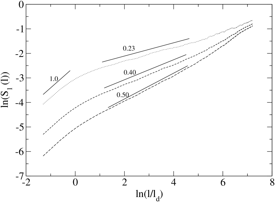
FIG. 1.: This figure plots $\ln(S_{1}(l))$ against $\ln(l/l_{d})$. Always $T=1$ and $\nu=5\times 10^{-7}$. Here $b=1.2$ for the dotted line, $b=0.9$ for the dashed line, and $b=0.5$ for the long-dashed line. The straight line above each curve shows the scaling behaviour, and the number over the line indicates its slope. The two regimes are observed: a) smooth (slope $1$ for $\ln(l/l_{d})<0$, b) scaling behaviour with slope $b/\lambda$ for $\ln(1)<\ln(l/l_{d})<<\ln(L/L_{d})=\ln(1/l_{d})$.

Next, we proceed to check numerically the validity of Eq.(39). First, we realize that, on dimensional grounds, the adimensional ratio $\overline{S}_{1}\equiv S_{1}(l)/S_{1}(l=l_{d})$ should be a function just of the adimensional parameters $l$, $l_{d}$, and $b/\lambda$. Expression (39) fully satisfies this requirement. This can be used to compare numerically-obtained values of $S_{1}$ as a function of $l$ (or $l/l_{d}$ as in the plot) for a variety of values of $\lambda$, $b$, and $\nu$ with the theoretical prediction. This last function would be a single curve as long as the combinations $l_{d}=2\sqrt{2\nu/\lambda}/L$ and $b/\lambda$ do not change. Figure (2) shows (for two different values of $(\nu/\lambda,b/\lambda)$) that the numerical data indeed scale as expected from the theory, and that the data collapse into the analytic curves is very good, confirming the accuracy of expression (39).

Finally, in Fig. (3) we perform an analogous plot (in logarithmic scale) to Fig. (2a) but for the power spectrum (also normalised to the diffusion length scale) analytically calculated by Corrsin (2), and the ones obtained numerically for the same values of $b$, $\lambda$ and $\nu$. Just a visual inspection confirms our expectation that, due to the effect of intermittency, it is more reliable to compare with numerical or real data the approximations to the first order structure function than the approximations to the power spectrum. Also, it is worth to mention that to calculate the power spectrum much more data are needed to obtain a nice statistics than in the case of the first order structure function.

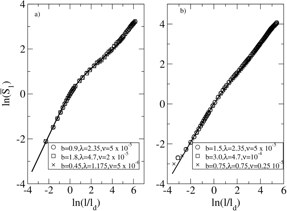
FIG. 2.: Plot of the adimensional structure function, $\overline{S}_{1}$, as a function of $l/l_{d}\equiv\delta x/L_{d}$. With solid line we plot the theoretical result (Eq.(39)), and with different symbols the different values obtained numerically. a) is for the fixed values $b/\lambda=0.382$ and $\nu/\lambda=4.2\times 10^{-6}$. b) the same for $b/\lambda=0.639$ and $\nu/\lambda=2.1\times 10^{-5}$. The symbols in the legends indicate the values of $b$, $\lambda$ and $\nu$ used to obtain the numerical data.

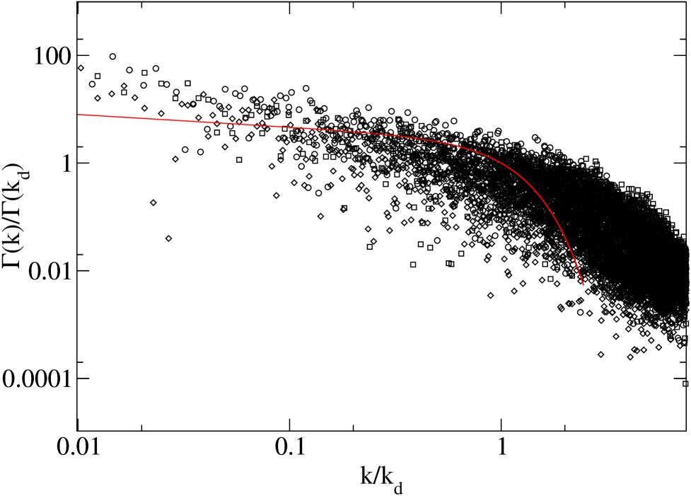
FIG. 3.: Comparison of the power spectrum (solid line) obtained by Corrsin (2) and numerical data as in Fig. (2a).

IV SUMMARY

To summarize, in this paper we have investigated the role of diffusion in the scaling properties of the first order structure function of a passive scalar chaotically advected. Based on the Feynman-Kac representation of the advection-reaction-diffusion equation, we have obtained an analytical expression for the the shape of the first order structure function for all scales smaller than the typical system size, and observed the existence of a crossover between a smooth regime and a scaling regime with slope depending on the rate of the decaying coefficient and the maximum Lyapunov exponent of the flow. The length-scale for the crossover is the typical dissipative length scale, given by $L_{d}=2\ \sqrt{\frac{2\nu}{\lambda}}$, which is independent of the decaying coeficient and, therefore, is the same as for the passive scalar with infinite lifetime. Moreover, our results confirm that the scaling exponent of $S_{1}$ are not modified by the molecular diffusion. We have shown that our approximation for the first order structure function is more reliable than the one for the power spectrum obtained under the same disregard of intermittency corrections. This could be relevant when explaining or modeling numerical or experimental data. We have also provided numerical support to our analytical findings. These are in excellent agreement. Our numerical algorithm uses the Feynman-Kac representation, and allows for a very fine scale resolution, as we just need to calculate the scalar field in one-dimensional sections of the whole surface. We believe that this numerical algorithm can be very useful for other kind of advection-reaction-diffusion problems.

V Acknowledgments

We acknowledge Zoltán Neufeld for his contributions to an early version of the Paper, and Angelo Vulpiani for suggesting us the use of the Feynmann-Kac formula. C.L. acknowledges financial support from the Spanish MECD. E.H-G acknowledges support from MCyT (Spain) projects BFM2000-1108 (CONOCE) and REN2001-0802-C02-01/MAR (IMAGEN).

REFERENCES

- [1] G. Károlyi, A. Péntek, I. Scheuring, T. Tél, and Z. Toroczkai, PNAS 97, 13661 (2000); S. Edouard, B. Legras, F. Lefèvre and R. Eymard, Nature, 384, 444 (1996); N. Peters, Turbulent combustion, Cambridge University Press (2000).
- [2] Z. Neufeld, C. López and P.H. Haynes, Phys. Rev. Lett. 82, 2606 (1999).
- [3] Z. Neufeld, C. López, E. Hernández-García and T. Tél, Phys. Rev. E 61, 3857 (2000).
- [4] H. Aref, J. Fluid Mech. 143, 1 (1984); A. Crisanti, M. Falcioni, G. Paladin and A. Vulpiani, Riv. Nuov. Cim. 14, 1 (1991).
- [5] E. Abraham, Nature 391, 577 (1998).
- [6] C. López, Z. Neufeld, E. Hernández-García and P.H. Haynes, Phys. Chem. Earth 26, 313 (2001); E. Hernández-García, C. López and Z. Neufeld, Chaos 12, 470 (2002).
- [7] P. H. Haynes, Transport, stirring and mixing in the atmosphere in Mixing: Chaos and Turbulence, H. Chaté and E. Villermaux (eds.), Kluwer, Dordretch (1999).
- [8] E. Abraham, A note on the wavenumber spectra of sea-surface temperature and chlorophyll, unpublished (1999).
- [9] K. Nam, E. Ott, T. M. Antonsen, Jr, and P. N. Guzdar, Phys. Rev. Lett. 84, 5134 (2000); G. Boffetta, A. Celani, S. Musacchio and M. Vergassola (unpublished), in nlin.CD/0111066.
- [10] S. Corrsin, J. Fluid Mech. 11, 407 (1961).
- [11] R.H. Kraichnan, Phys. Fluids 11, 945 (1968).
- [12] G. K. Batchelor, J. Fluid Mech. 5, 113 (1959).
- [13] K. Nam, T. M. Antonsen, Jr., P.N. Guzdar and E. Ott, Phys. Rev. Lett. 83, 3426 (1999).
- [14] M. Chertkov, Phys. Fluids 10, 3017 (1998); M. Chertkov, Phys. Fluids 11, 2257 (1999).
- [15] T. Bohr, M. Jensen, G. Paladin and A. Vulpiani, Dynamical Systems Approach to Turbulence, Cambridge Univ. Press, Cambridge, 1998.
- [16] M. Freidlin, Markov Processes and Differential Equations, Birkhauser, Boston (1996).
- [17] G. Falkovich, K. Gawedzki and M. Vergassola, Rev. Mod. Phys. 73, 913 (2001).
- [18] Goldhirsch et al. Physica D 27, 311 (1987).
- [19] M. San Miguel, E. Hernández-García, P. Colet, M.O. Caceres, F. De Pasquale, in Instabilities and Nonequilibrium Structures III, Eds. E. Tirapegui and W. Zeller, Kluwer (1991), and references therein.
- [20] M. Abramowitz and I.A. Stegun, Handbook of Mathematical Functions, Applied Mathematics Series, vol.55, Dover Publications, New York, 1964.