Starting with the general description of a moving curve, we have recently presented a unified formalism to show that three distinct space curve evolutions can be identified with a given integrable equation. Applying this to the nonlinear Schrödinger equation (NLS), we find three sets of coupled equations for the evolution of the curvature and the torsion, one set for each moving curve. The first set is given by the usual Da Rios-Betchov equations. The velocity at each point of the curve that corresponds to this set is well known to be a local expression in the curve variables. In contrast, the velocities of the other two curves are shown to be nonlocal expressions. Each of the three curves is endowed with a corresponding infinite set of geometric constraints. These moving space curves are found by using their connection with the integrable Landau- Lifshitz equation. The three evolving curves corresponding to the envelope soliton solution of the NLS are presented and their behaviors compared.

 

${}^{1}~{}{\small\rm The~{}~{}Institute~{}~{}of~{}~{}Mathematical~{}~{}sciences,~{}~{}Chennai~{}~{}600~{}113,~{}~{}India.}$

1 Introduction

The study of possible links between intrinsic kinematics of space curves [1] and integrable soliton bearing equations[2] deserves attention because of a wide variety of applications of moving curves such as vortex filament motion in fluids [3], dynamics of continuum spin chains [4], scroll waves in chemical reactions [5], superfluids [6], interface dynamics [7], etc. The pioneering work by Hasimoto [3] on the motion of a vortex filament in a fluid was the first to suggest such a link. In classical differential geometry, a space curve embedded in three dimensions is described using the following Frenet-Serret equations [1] for the orthonormal triad of unit vectors made up of its tangent ${\bf t}$, normal ${\bf n}$ and the binormal ${\bf b}$:

$${\bf t}_{s}\ =\ K{\bf n}\ ;\ {\bf n}_{s}\ =\ -K{\bf t}\ +\ \tau{\bf b}\ ;\ {\bf b}_{s}\ =\ -\tau{\bf n}.$$ (1.1)

Here, $s$ denotes the arclength. The parameters $K$ and $\tau$ represent the curvature and torsion of the space curve. For a moving curve, these will be functions of both $s$ and time $u$. The subscript $s$ denotes partial derivative.

Using the so-called local induction approximation, Da Rios [8] showed that the curve velocity ${\bf v}(s,u)$ at each point $s$ of a vortex filament (regarded as a moving space curve) is given by the local induction equation :

$${\bf v}={\bf r}_{u}=~{}~{}K~{}{\bf b}$$ (1.2)

For non-stretching curves, using compatibility conditions ${\bf r}_{us}={\bf r}_{su}={\bf t}_{u}=K_{s}{\bf b}-K\tau{\bf n}$, along with similar compatibility conditions for ${\bf t}$ and ${\bf n}$ leads to [8]

$$K_{u}=-(K\tau)_{s}-K_{s}\tau;~{}~{}\tau_{u}=[(K_{ss}/K)-\tau^{2}]_{s}-KK_{s}.$$ (1.3)

Subsequently, the above coupled equations for $K$ and $\tau$ were also derived independently by Betchov [9], and hence Eq. (1.3) is referred to as Da Rios-Betchov (DB) equations. Connection between these curve equations and solitons was unravelled by Hasimoto [3], whose analysis essentially showed that by using the following ‘Hasimoto function’

$$\psi=~{}~{}K~{}~{}\exp[i\int~{}\tau~{}~{}ds],$$ (1.4)

the two equations in (1.3) can in fact be combined to give the integrable, soliton-bearing nonlinear Schrödinger equation (NLS)

$$iq_{u}+q_{ss}+\frac{1}{2}~{}|q|^{2}~{}q=0,$$ (1.5)

with $q=\psi$. Motivated by this result, Lamb [10] gave a general procedure which helps identify a certain space curve evolution with a given integrable equation. Examples such as the NLS, the sine-Gordon equation and the modified KdV equation were considered. Recently, we presented [11] a unified analysis to show that in general, two more distinct curve evolutions can also be so identified. In this paper, after outlining this analysis, we specialize to the NLS, and focus on the intrinsic kinematics of the three moving curves associated with it. We obtain coupled evolution equations for the curvature and torsion of each of the two new curves. These are certain analogs of the DB equations (1.3). Each of the three moving curves is shown to be endowed with an infinite set of geometric invariants. Their natural connection with the integrable Landau-Lifshitz equation is pointed out, and a procedure to use its solution to construct the position vectors generating the three curves associated with the NLS is given. As an example, the moving curves for an envelope soliton solution of the NLS are found, and their behaviors compared. Interestingly, the velocities (at every point) of the two new moving curves underlying the general NLS evolution turn out to be certain nonlocal functions of the curve variables, quite in contrast to the local expression (Eq. (1.2)) for the velocity of the usual moving curve that has thus far been associated with the NLS. Possible application of these results to vortex filament motion in fluids is suggested.

2 Identification of three curve evolutions with a given integrable equation

To describe a moving curve, we find it convenient to introduce [12] the following time evolution equations for the Frenet triad $({\bf t},{\bf n},{\bf b})$:

$${\bf{t}}_{u}\,=g{\bf{n}}+h{\bf{b}}\ ;\ {\bf{n}}_{u}\,=-g{\bf{t}}+\tau_{0}{\bf{b}}\ ;\ {\bf{b}}_{u}\,=\,-h{\bf{t}}-\tau_{0}{\bf{n}}.$$ (2.1)

The parameters $g,h$ and $\tau_{0}$ are, at this stage, general parameters which determine the time evolution of the curve. They are functions of both $s$ and $u$. The subscript $u$ stands for partial derivative. On imposing the compatibility conditions

$${\bf t}_{su}\ =\ {\bf t}_{us}\ ;\ {\bf n}_{su}\ =\ {\bf n}_{us}\quad;\quad{\bf b}_{su}\ =\ {\bf b}_{us},$$ (2.2)

and using Eqs. (1.1) and (2.1), we obtain

$$K_{u}=(g_{s}-\tau h);~{}~{}\tau_{u}=(\tau_{0})_{s}+Kh;~{}~{}h_{s}=(K\tau_{0}-\tau g).$$ (2.3)

Lamb’s procedure [10] will be referred to as ”formulation (I)”, to distinguish it from two other additional formulations that are possible [11]. We shall use the subscripts $1,2$ and $3$ on the various curve parameters appearing in the three formulations, for ready reference.
Formulation I: Here, one combines the second and third of Eqs. (1.1), which immediately suggests the definition of a complex vector ${\bf N}=({\bf n}+i{\bf b})~{}~{}{\rm exp}[i\int\tau~{}ds]$, along with the complex function $\psi$ given in Eq. (1.4). By writing ${\bf N}_{s},{\bf t}_{s},{\bf N}_{u}$ and ${\bf t_{u}}$ in terms of ${\bf t}$ and ${\bf N}$, imposing the compatibility condition ${\bf N}_{su}\ =\ {\bf N}_{us}$, and equating the coefficients of t and N in it, one obtains

$$\psi_{u}+\gamma_{1s}+(1/2)[\int~{}(\gamma_{1}\psi^{*}-\gamma_{1}^{*}\psi)~{}~{}ds]~{}\psi=0.$$ (2.4)

where

$$\gamma_{1}=-(g+ih)~{}~{}{\rm exp}[i\int\tau~{}ds].$$ (2.5)

Thus for an appropriate choice of $\gamma_{1}$ as a function of $\psi$ and its derivatives, a known integrable equation for $\psi$ can be obtained from (2.4). Then, by comparing a known solution of this equation with the Hasimoto function (1.4), the curvature $K$ and torsion $\tau$ of the corresponding moving space curve can be found. Next, using the above mentioned specific choice of $\gamma_{1}$ in Eq. (2.5), the curve evolution parameters $g$ and $h$ can be determined as some specific functions of $K$ ,$\tau$ and their derivatives. Armed with these, $\tau_{0}$ can also be found from the third equation in (2.3). Thus a set of curve parameters $K$, $\tau$, $g$, $h$ and $\tau_{0}$ has been found explicitly. In other words, a certain moving curve described by these parameters has thus been identified with a given solution of the integrable equation for $\psi$.

As already mentioned, we have recently shown [11] that in addition to the above, there are two other distinct curves that can be identified with a given integrable equation. The procedures leading to these curves will be called formulations (II) and (III), respectively.
Formulation (II): Combining the first two equations in (1.1) appropriately, we see that a complex vector ${\bf M}=({\bf n}-i{\bf t})~{}{\rm exp}[i\int K~{}ds]$ and a complex function

$$\Phi(s,u)=\tau\exp{[i\int K~{}ds]},$$ (2.6)

appear. Proceeding in a fashion analogous to (I) above, and imposing ${\bf M}_{su}={\bf M}_{us}$, we get

$$\Phi_{u}+\gamma_{2s}+(1/2)[\int~{}(\gamma_{2}\Phi^{*}-\gamma_{2}^{*}\Phi)~{}~{}ds]~{}\Phi=0.$$ (2.7)

where

$$\gamma_{2}=-(\tau_{0}-ih)~{}~{}{\rm exp}[i\int K~{}ds].$$ (2.8)

Formulation (III): Here, we combine the first and third equations of (1.1), leading to the appearance of a complex vector ${\bf P}=({\bf t}-i{\bf b})$, and a complex function $\chi$ given by

$$\chi(s,u)=(K+i\tau).$$ (2.9)

On requiring ${\bf P}_{su}={\bf P}_{us}$, we get

$$\chi_{u}+\gamma_{3s}+(1/2)[\int~{}(\gamma_{3}\chi^{*}-\gamma_{3}^{*}\chi)~{}~{}ds]~{}\chi=0.$$ (2.10)

where

$$\gamma_{3}=-(g+i\tau_{0}).$$ (2.11)

Now, Eqs. (2.7) and (2.10) have the same form as Lamb’s equation (2.4). The discussion in the paragraph following Eq. (2.5) makes it clear that for an appropriate choice of $\gamma_{2}$ as a function of $\Phi$ and its derivatives, and of $\gamma_{3}$ as a function of $\chi$ and its derivatives, known integrable equations for $\Phi$ and $\chi$ can be obtained from these equations.

It is important to note from Eqs. (1.4), (2.6) and (2.9) that the complex functions $\psi$, $\Phi$ and $\chi$ that satisfy the (same) integrable equation in the three formulations are different functions of $K$ and $\tau$. Further, we see that the complex quantities $\gamma_{1}$, $\gamma_{2}$ and $\gamma_{3}$ (Eqs. (2.5), (2.8) and (2.11)) that arise in the three formulations respectively, also involve different combinations of the curve evolution parameters $g,h$ and $\tau_{0}$. Thus it is clear that the three formulations yield different sets of curve parameters, and hence describe three distinct moving space curves that can be associated with a given solution of an integrable equation. (We remark that it should be possible to extend our analysis to include partially integrable equations as well.) In the next section, we apply these results to the NLS, to demonstrate this clearly.

3 The NLS : Two analogs of Da Rios-Betchov equations

From the three formulations discussed in the last section, it can be easily verified that the respective choices

$$\gamma_{1}=-i\psi_{s};~{}~{}\gamma_{2}=-i\Phi_{s};~{}~{}\gamma_{3}=-i\chi_{s},$$ (3.1)

when used in Eqs. (2.4), (2.7) and (2.10) lead to the NLS given in (1.5), with $q$ identified with the three complex functions $\psi,\Phi$ and $\chi$, respectively. Since the NLS is a completely integrable equation [2], it possesses an infinite set of conserved quantities $I_{k},~{}k=1,2....\infty$, which are in involution pairwise. The first three of these invariants are given by [13]

$$I_{1}=\int~{}~{}|q|_{s}^{2}~{}~{}ds;~{}I_{2}=~{}~{}(1/2i)\int~{}~{}(q_{s}q^{*}~{}-~{}q_{s}q^{*})~{}~{}ds;~{}I_{3}=\int~{}[|q_{s}|^{2}~{}-~{}\frac{1}{4}|q|^{2}]~{}ds;....$$ (3.2)

Let us consider the implications of this in the three formulations:
(I) Setting $q=\psi$ in (1.5) and equating real and imaginary parts leads to DB equations (1.3). Therefore these also possess an infinite number of conserved quantities, obtained by setting $q=\psi$ in Eq. (3.2). The invariants now appear as geometric constraints [14]:

$$I_{1}=\int~{}K^{2}~{}~{}ds;~{}I_{2}=\int~{}K^{2}~{}\tau~{}~{}ds;~{}I_{3}=\int~{}[K_{s}^{2}+K^{2}\tau^{2}-~{}\frac{1}{4}K^{4}]~{}~{}ds;....$$ (3.3)

Further, an inspection of Eqs. (1.3) shows that the total torsion $I_{0}=\int~{}\tau~{}ds$ is also conserved. This additional geometric constraint has no counterpart among the NLS invariants given in (3.2).
(II) Here, we set $q=\Phi$ in (1.5) to yield the coupled equations

$$K_{u}=[(\tau_{ss}/\tau)-K^{2}]_{s}-\tau\tau_{s};~{}~{}\tau_{u}=-(K\tau)_{s}-\tau_{s}K.$$ (3.4)

This is the first analog of the DB equations (1.3). As is obvious from comparing $\psi$ in (1.4) and $\Phi$ in Eq.(2.6), this analog may be found by simply interchanging $K$ and $\tau$ in (1.3). Thus the associated infinite number of geometric constraints can also be found using this interchange in Eq. (3.3):

$$I_{1}=\int~{}\tau^{2}~{}~{}ds;~{}I_{2}=\int~{}\tau^{2}~{}K~{}~{}ds;~{}I_{3}=\int~{}[\tau_{s}^{2}+\tau^{2}K^{2}-~{}\frac{1}{4}\tau^{4}]~{}~{}ds;....$$ (3.5)

Here, the total curvature $I_{0}=\int~{}K~{}ds$ is also conserved. This has no counterpart among the conserved densities (3.2) of the NLS equation.
(III) Finally, setting $q=\chi$ in (1.5) yields the following second analog of the DB equations:

$$K_{u}=-\tau_{ss}-\frac{1}{2}(K^{2}+\tau^{2})\tau;~{}~{}\tau_{u}=K_{ss}+\frac{1}{2}(K^{2}+\tau^{2})K.$$ (3.6)

Next, setting $q=\chi$ in Eq. (3.2), we get the third set of infinite geometric constraints:

$$I_{1}=\int(K^{2}~{}+\tau^{2})~{}ds;~{}I_{2}=\int(K_{s}\tau~{}-K\tau_{s})~{}ds;~{}I_{3}=\int[K_{s}^{2}+\tau_{s}^{2}-\frac{1}{4}(K^{2}+\tau^{2})]~{}ds;....$$ (3.7)

We end this section with the remark that the total length of the curve, $L~{}=~{}\int~{}ds$ is also conserved in all three formulations, since the curves are non-stretching.

4 Construction of the three curves using
the Landau-Lifshitz equation

A general solution of the NLS (Eq. (1.5)) is of the form $q=\rho\exp[i\theta]$. Equating this with the three complex functions defined in Eqs.(1.4), (2.6) and (2.9) will yield the curvature and the torsion of the three space curves to be ${\bf(I)}~{}\kappa_{1}=\rho,~{}~{}\tau_{1}={\theta}_{s},~{}~{}{\bf(II)}~{}\kappa_{2}={\theta}_{s},~{}~{}\tau_{2}=\rho$ and ${\bf(III)}~{}\kappa_{3}=\rho\cos\theta,~{}~{}\tau_{3}=\rho\sin\theta$. These are clearly, three distinct space curves, each with a known curvature and torsion. However, solving the Frenet-Serret equations (1.1) explicitly for ${\bf t}$ by using these, to subsequently construct the position vector ${\bf r}(s,u)=\int{\bf t}~{}~{}ds$ of the (evolving) space curve, is a nontrivial task in practice. In the present context, we shall show that there is a certain link between the three curve evolutions and the integrable Landau Lifshitz (LL) equation [17], which provides us with an alternative procedure to construct the three moving curves.

We proceed by first equating the expressions for $\gamma_{1}$, $\gamma_{2}$ and $\gamma_{3}$ given in Eq. (3.1) with those given in Eqs. (2.5), (2.8) and (2.11). This yields the following curve evolution parameters $g,h$ and $\tau_{0}$ in the three cases:

$${\bf(I)}~{}~{}g_{1}=-\kappa_{1}\tau_{1};~{}~{}h_{1}=\kappa_{1s};~{}~{}\tau_{01}=(\kappa_{1ss}/\kappa_{1})-\tau_{1}^{2},$$ (4.1)

$${\bf(II)}~{}~{}g_{2}=(\tau_{2ss}/\tau_{2})-\kappa_{2}^{2};~{}~{}h_{2}=-\tau_{2s};~{}~{}\tau_{02}=-\kappa_{2}\tau_{2},$$ (4.2)

$${\bf(III)}~{}~{}g_{3}=-\tau_{3s};~{}~{}~{}h_{3}=(1/2)(\kappa_{3}^{2}+\tau_{3}^{2});~{}~{}\tau_{03}=\kappa_{3s}.$$ (4.3)

Substituting these expressions for each of the formulations appropriately in Eqs. (2.1), and using Eq. (1.1), a short calculation [11] shows that the completely integrable LL equation [17]

$${\bf S}_{u}={\bf S}\times{\bf S}_{ss};~{}~{}~{}{\bf S}^{2}=1$$ (4.4)

is obtained in every case, i.e., Eq. (4.4) is satisfied by the tangent ${\bf t}_{1}$ of the moving space curve in the first formulation, by the binormal ${\bf b}_{2}$ in the second, and the normal ${\bf n}_{3}$ in the third [18]. Of the above, the first may be regarded as the converse of Lakshmanan’s mapping [4] where, starting with the LL equation, and identifying ${\bf S}$ with the tangent to a moving curve, one obtained the DB equations, and from them, the NLS for $\psi$. The converses of the other two will yield the two analogs of the DB equations obtained in Section 3, and clearly lead to new geometries connected with the NLS.

The LL equation (4.4) has been shown to be completely integrable [19] and gauge equivalent[20] to the NLS. Its exact solutions can be found [19, 21]. We now outline [22] how ${\bf r}_{1}$, ${\bf r}_{2}$ and ${\bf r}_{3}$, the position vectors generating the three moving curves underlying the NLS, can be found in terms of an exact solution ${\bf S}$ of Eq. (4.4). Let $({\bf t}_{i},{\bf n}_{i},{\bf b}_{i})$, $i=1,2$ and $3$, respectively, denote the Frenet triads of the three moving curves satisfying Eqs. (1.1), with the corresponding parameters $\kappa_{i}$ and $\tau_{i}$.
(I) Here, ${\bf t}_{1}={\bf r}_{1s}$ is the tangent to a certain moving curve created by a position vector ${\bf r}_{1}(s,u)$. Here, we set ${\bf t}_{1}={\bf S}$, a known solution of Eq. (4.4).Thus

$$\kappa_{1}=|{\bf t}_{1s}|=|{\bf S}_{s}|;~{}~{}\tau_{1}=\frac{{\bf t}_{1}.({\bf t}_{1s}\times{\bf t}_{1ss})}{{\bf t}^{2}_{1s}}=\frac{{\bf S}.({\bf S}_{s}\times{\bf S}_{ss})}{{\bf S}^{2}_{s}}$$ (4.5)

Thus the underlying moving curve ${\bf r}_{1}(s,u)$ is given by

$${\bf r}_{1}(s,u)=\int{{\bf t}_{1}~{}ds}=\int{{\bf S}(s,u)~{}ds}$$ (4.6)

The above expression for ${\bf r}_{1}$ coincides with the surface that one would obtain using Sym’s [16] soliton-surface method.
(II) Here, ${\bf b}_{2}$ is the binormal of some moving curve ${\bf r}_{2}(s,u)$. We set ${\bf b}_{2}={\bf S}$. We have, ${\bf t}_{2}={\bf r}_{2s}$. The curvature $\kappa_{2}=\tau_{1}$ and torsion $\tau_{2}=\kappa_{1}$ (See Eq.(4.5)). The position vector ${\bf r}_{2}(s,u)$ generating the moving curve can be shown to be [22]

$${\bf r}_{2}(s,u)=\int{{\bf t}_{2}~{}ds}=\int{{\bf S}_{s}\times\frac{{\bf S}}{\kappa_{1}}~{}~{}ds}$$ (4.7)

(III) Here, ${\bf n}_{3}$ the normal of some other moving curve ${\bf r}_{3}(s,u)$. Thus we set ${\bf n}_{3}={\bf S}$. Further, ${\bf t}_{3}={\bf r}_{3s}$. Next, from the Frenet-Serret equations (1.1) for this triad,

$$(\kappa_{3}^{2}+\tau_{3}^{2}){\bf t}_{3}=\tau_{3}({\bf n}_{3}\times{\bf n}_{3s})-\kappa_{3}{\bf n}_{3s}$$ (4.8)

A short calculation shows [22] that $\kappa_{3}=\kappa_{1}\cos\eta_{1}$ and $\tau_{3}=\kappa_{1}~{}~{}\sin\eta_{1}$, where $\eta_{1}=[\int\tau_{1}~{}~{}ds~{}~{}+~{}~{}c_{1}(u)]$. Here, $c_{1}(u)$ is a function of time $u$, which can be determined in terms of $\kappa_{1}$ and $\tau_{1}$, after a short calculation, by using the equations for $\kappa_{3u}$ and $\tau_{3u}$ obtainable from Eqs. (2.3). Then, substituting the values for $\kappa_{3}$ and $\tau_{3}$ into Eq. (4.8), and setting ${\bf n}_{3}={\bf S}$, the position vector ${\bf r}_{3}(s,u)$ creating the third moving space curve can be found to be [22]

$${\bf r}_{3}(s,u)=\int{\bf t}_{3}~{}ds=\int\frac{[({\bf S}\times{\bf S}_{s})\sin\eta_{1}-{\bf S}_{s}~{}~{}\cos\eta_{1}])}{\kappa_{1}}~{}ds$$ (4.9)

5 Moving space curves associated with the NLS soliton.

As seen in the last section, the expressions for the three moving curves associated with the NLS are given in (4.6), (4.7) and (4.9) respectively, in terms of a known solution ${\bf S}$ of the LL equation (4.6). By defining three orthogonal unit vectors ${\bf\hat{e}}_{1}=\Big{\{}1,0,0\Big{\}},~{}{\bf\hat{e}}_{2}=\Big{\{}0,\cos\eta,\sin\eta\Big{\}},~{}{\bf\hat{e}}_{3}=\Big{\{}0,-\sin\eta,\cos\eta\Big{\}}$, a soliton solution [21] of (4.6) can be written in the form

$${\bf S}(s,u)=(1-\mu\nu{\rm sech}^{2}(\nu\xi)){\bf\hat{e}}_{1}+\mu\nu{\rm sech}(\nu\xi)\tanh(\nu\xi){\bf\hat{e}}_{2}-\mu\lambda{\rm sech}(\nu\xi){\bf\hat{e}}_{3},$$ (5.1)

where, $\xi=(s-2\lambda u),~{}\eta=(\lambda s+(\nu^{2}-\lambda^{2})u)$ and $\mu=2\nu/(\nu^{2}+\lambda^{2})$. Here, $\nu$ and $\lambda$ denote arbitrary constants. As is clear from our discussion in Section 4, the three curves that result from this solution are associated with the soliton solution $q=2\nu{\rm sech}(\nu\xi)~{}\exp{(i\eta)}$ of the NLS (Eq. (1.5)). They are found as follows:
(I)  Substituting Eq. (5.1) in Eq. (4.5), we get $\kappa_{1}=2\nu{\rm sech}(\nu\xi)$ and $\tau_{1}=\lambda.$ Next, substituting Eq. (5.1) in Eq. (4.6) yields

$${\bf r}_{1}=\Big{(}s-\mu\tanh(\nu\xi),-\mu{\rm sech}(\nu\xi)\cos\eta,-\mu{\rm sech}(\nu\xi)\sin\eta\Big{)}$$ (5.2)

This is seen to agree with the result obtained in [15] using Sym’s [16] procedure. In Fig. (1), we have presented a stroboscopic plot of the moving curve (5.2) at different instants of time. This describes the propagation of the well known Hasimoto ”loop” soliton. In between the times at which we have plotted the curve, the loop changes its size and also rotates about the asymptotic direction which the curve takes on at $s\rightarrow\pm~{}\infty$. In the figure, we have not plotted these intermediate times for the sake of clarity. The loop regains its form at subsequent times, as we see from the figure.
(II)  Here, we get $\kappa_{2}=\lambda$ and $\tau_{2}=2\nu{\rm sech}(\nu\xi)$. Substituting Eq. (5.1) in Eq. (4.7), the moving curve is found to be

$${\bf r}_{2}=\int[\mu\lambda{\rm sech}(\nu\xi){\bf\hat{e}}_{1}-\mu\lambda\tanh(\nu\xi){\bf\hat{e}}_{2}+\frac{(\lambda^{2}-\nu^{2})}{(\lambda^{2}+\nu^{2})}{\bf\hat{e}}_{3}]~{}ds$$ (5.3)

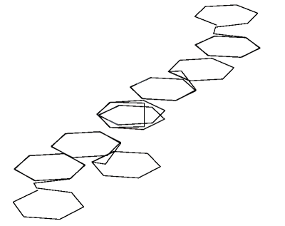
Figure 2: A stroboscopic plot of the evolving space curve ${\bf r}_{2}(s,u)$ (Eq. (5.3)) for $\nu=0.3$ and $\lambda=0.1$.

In this case, since the curvature is constant and the torsion vanishes as $s\rightarrow\pm\infty$, for all finite times, the curve is bounded by two planar circles at both ends. The maximum non-planarity of the curve occurs at $s=2\lambda u$. A stroboscopic plot of Eq. (5.3) given in Fig. (2). This curve is clearly seen to rotate and propagate as time progresses.
(III)  Here, $\kappa_{3}=2\nu{\rm sech}(\nu\xi)\cos\eta$ and $\tau_{3}=2\nu{\rm sech}(\nu\xi)\sin\eta$. When Eq. (5.1) is substituted in Eq. (4.9), with $\eta_{1}=\eta$, a long but straightforward calculation yields

$${\bf r}_{3}=\int[\mu{\rm sech}(\nu\xi)(\lambda\sin\eta-\nu\tanh(\nu\xi)\cos\eta){\bf\hat{e}}_{1}{}$$ (5.4)

$${}-(\mu\lambda\tanh(\nu\xi)\sin\eta+(1-\mu\nu\tanh^{2}(\nu\xi))\cos\eta){\bf\hat{e}}_{2}{}$$

$${}+(\frac{(\lambda^{2}-\nu^{2})}{(\lambda^{2}+\nu^{2})}\sin\eta-\mu\lambda\tanh(\nu\xi)\cos\eta){\bf\hat{e}}_{3}]~{}ds$$

A stroboscopic plot of the moving curve (5.4) at different instants of time is given in Fig. (3). This depicts the propagation of a ”loop” soliton distinct from the Hasimoto soliton in the sense that it also oscillates with time, as is clear from the figure. Furthermore, at intermediate times, the loop rotates about the asymptotic direction, decreasing its loop size, and almost straightens out periodically, after which it starts looping again. These intermediate plots have not been presented in the figure.

6 Three curve velocities associated with NLS evolution

Returning to our general results of Section 4, the three position vectors ${\bf r}_{i}$, $i=1,2$ and $3$, which are associated with the NLS evolution, can be found from Eqs. (4.6), (4.7) and (4.9), respectively, using an exact solution${\bf S}$ of the LL equation (4.4). The corresponding curve velocities ${\bf v}_{i}(s,u)={\bf r}_{iu}$ at each point $s$, can therefore be found from these equations by direct differentiation with respect to time, $u$. However, to compare and contrast the intrinsic geometries of the three space curves, it is instructive to express these velocities in terms of the vectors of the corresponding Frenet triads, as well as the curve parameters, as follows. Since the curves are non-stretching, we have ${\bf v}_{is}={\bf r}_{ius}={\bf r}_{isu}={\bf t}_{iu}$. On the other hand, from the first equation of Eqs. (2.1), we have, ${\bf t}_{iu}=g_{i}{\bf n}_{i}+h_{i}{\bf b}_{i}$. Here, the quantities $g_{i}$ and $h_{i}$ for the three curves of the NLS are given in Eqs. (4.1), (4.2) and (4.3), respectively. Using these in ${\bf v}_{i}(s,u)=~{}\int~{}{\bf t}_{iu}~{}~{}ds$, we get

$${\bf(I)}~{}~{}{\bf v}_{1}=~{}\int(-\kappa_{1}\tau_{1}{\bf n}_{1}+\kappa_{1s}{\bf b}_{1})~{}ds=~{}\kappa_{1}~{}{\bf b}_{1}.$$ (6.1)

$${\bf(II)}~{}~{}{\bf v}_{2}=~{}\int~{}[(\tau_{2ss}/\tau_{2}-~{}\kappa_{2}^{2}){\bf n}_{2}-\kappa_{2s}{\bf b}_{2}]~{}ds.$$ (6.2)

$${\bf(III)}~{}~{}{\bf v}_{3}=~{}\int~{}[-\tau_{3s}{\bf n}_{3}+~{}\frac{1}{2}(\kappa_{3}^{2}+\tau_{3}^{2}){\bf b}_{3}]~{}ds.$$ (6.3)

As expected, ${\bf v}_{1}$ coincides with the vortex filament velocity Eq. (1.2) derived by Da Rios in fluid mechanics. It is a local expression in the curve variables: The velocity ${\bf v}_{1}$ at a point $s$ depends on the curvature and binormal at that point only. In contrast, ${\bf v}_{2}$ and ${\bf v}_{3}$ are seen to be nonlocal in the curve variables: If we partially integrate the right hand sides of Eqs. (6.2) and (6.3), and use the Frenet-Serret equations (Eqs. (1.1)) repeatedly in the resulting expressions, both these velocities take on the form ${\bf v}_{i}=A_{i}~{}{\bf t}_{i}+~{}B_{i}~{}{\bf n}_{i}+~{}C_{i}~{}{\bf b}_{i}$, $i=2,3$, where the components $A_{i},B_{i}$ and $C_{i}$ can be written in terms of integrals of certain functions involving the curvature, the torsion , their higher derivatives, and their various products. It is indeed interesting that in spite of such a complicated behaviour of these velocities, their corresponding curve evolutions are also endowed with an infinite number of constants of motion. This essentially stems from their connection with the NLS. More specifically, this is because, as we have shown in Section 3, the binormal ${\bf b}_{2}$ of the second curve and the normal ${\bf n}_{3}$ of the third, satisfy the integrable LL equation.

We conclude with the following remarks: In a fluid, as is well known, the induced velocity ${\bf v}$ at a point is determined as a volume integral involving the vorticity ${\bf\Omega}$, by using the Biot-Savart formula. First, it is to be noted that in this formula, if one expresses ${\bf\Omega}$ in terms of the vectors of the Frenet triad of the filament, then, in any realistic model of a fluid, ${\bf v}$ is nonlocal in the curve variables, and becomes local only under certain approximations. Secondly, it is worth noting that in an interesting experiment with a fluid in a rotating tank, Hopfinger and Browand [23] had observed compact distortions which twist and propagate along a vortex core like a soliton. These two features suggest that our new results which link the velocities ${\bf v}_{2}$ and ${\bf v}_{3}$ with the NLS and its soliton, may be of some relevance in actual fluids. In view of this, appropriate theoretical modeling of the vorticity, as well as possible experimental studies of the detailed geometric structure of moving vortex filaments, to look for any similarities with Figures (1) to (3) (which depict propagation of compact distortions) would indeed be of interest.

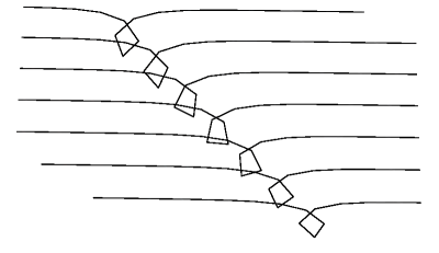
Figure 1: A stroboscopic plot of the evolving space curve ${\bf r}_{1}(s,u)$ (Eq. (5.2)) for $\nu=1$ and $\lambda=0.1$.

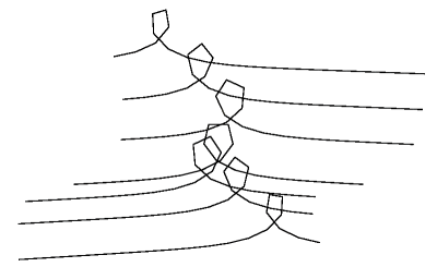
Figure 3: A stroboscopic plot of the evolving space curve ${\bf r}_{3}(s,u)$ (Eq. (5.4)) for $\nu=1$ and $\lambda=0.3$.

References

- [1] See, for instance, D. J. Struik, Lectures on Classical Differential Geometry (Addison-Wesley, Reading, MA 1961).
- [2] See, for instance, M. J. Ablowitz and H. Segur, Solitons and the Inverse Scattering Transform, ( SIAM, Philadelphia,1981).
- [3] H. Hasimoto, J. Fluid. Mech. 51, 477 (1972).
- [4] M. Lakshmanan, Phys. Lett. A 61, 53 (1977); Radha Balakrishnan, J. Phys. C 15, L1305 (1982).
- [5] J. P. Keener, Physica D 31, 269 (1998) and references therein.
- [6] K. W. Schwarz, Phys. Rev. B 38, 2398 (1998).
- [7] R. E. Goldstein and D. M. Petrich, Phys. Rev Lett. 67, 3203 (1991).
- [8] L. S. Da Rios, Rend. Circ. Mat. Palermo 22, 117 (1906).
- [9] R. Betchov, J. Fluid Mech. 22, 471 (1965); For history, see R. L. Ricca, Nature 352, 561 (1991).
- [10] G.L. Lamb, J. Math. Phys. 18, 1654 (1977) .
- [11] S. Murugesh and Radha Balakrishnan, Phys. Lett. A 290, 81 (2001); nlin. PS/0104066.
- [12] Radha Balakrishnan, A. R. Bishop, R. Dandoloff, Phys. Rev. B 47, 3108 (1993); Phys. Rev. Lett. 64, 2107 (1990); Radha Balakrishnan and R. Blumenfeld, J. Math. Phys. 38, 5878 (1997).
- [13] Here, is the Hamiltonian which gives rise to (1.5), on using the Poisson brackets .
- [14] J. Langer and R. Perline, J. Math. Phys. 35, 1732 (1993).
- [15] D. Levi, A. Sym and S. Wojciechowski, Phys. Lett. A 94, 408 (1983).
- [16] A.Sym, Lett. Nuovo Cimento 22, 420 (1978) .
- [17] L.D. Landau and E. M. Lifshitz, Phys. Z Sowjet 8, 153 (1935).
- [18] The Hamiltonians for these three evolutions are just the respective invariants given in Eqs. (3.3), (3.5) and (3.7). These can be written in the form , with the spin vector identified with and , respectively. Thus the components of each of these three vectors satisfy the usual angular momentum Poisson brackets.
- [19] L.A. Takhtajan, Phys. Lett. A 64, 235 (1977).
- [20] V. E. Zakharov and L. A. Takhtajan, Theor. Math. Phys. 38, 26 (1979).
- [21] J. Tjon and J. Wright, Phys. Rev. B 15, 3470 (1977).
- [22] S. Murugesh and Radha Balakrishnan, Euro. Phys. Jour. B (submitted).
- [23] E. J. Hopfinger and F. K. Browand, Nature 295, 393 (1982).