Abstract

We use the Riemann-Hilbert problem to study the interaction of the soliton with radiation in the parametrically driven, damped nonlinear Schrödinger equation. The analysis is reduced to the study of a finite-dimensional dynamical system for the amplitude and phase of the soliton and the complex amplitude of the long-wavelength radiation. In contrast to previously utilised Inverse Scattering-based perturbation techniques, our approach is valid for arbitrarily large driving strengths and damping coefficients. We show that, contrary to suggestions made in literature, the complexity observed in the soliton’s dynamics cannot be accounted for just by its coupling to the long-wavelength radiation.

1 Introduction

A variety of nonlinear wave phenomena in one dimension can be modelled by the perturbed nonlinear Schrödinger (NLS) equation:

$$iq_{t}+q_{xx}+2|q|^{2}q={\cal R}(t,x,q,q^{*},q_{x},q^{*}_{x},...).$$ (1)

(Here and below the asterisk denotes complex conjugation.) The present paper deals with the parametrically driven, damped NLS, for which

$${\cal R}=he^{2i\Omega_{0}t}q^{*}-i\gamma q;\quad h,\;\Omega_{0},\;\gamma>0.$$ (2)

This equation describes nonlinear Faraday resonance in a vertically oscillating water trough [1, 2, 3, 4, 5, 6, 7, 8, 9, 10, 11, 12]; an easy-plane ferromagnet with a combination of a stationary and a high-frequency magnetic field in the easy plane [13]; and the effect of phase-sensitive amplifiers on solitons propagating in optical fibres [14, 15, 16].

The equation (1)-(2) has two stationary soliton solutions, one of which is unstable for all $h$ and $\gamma$ and hence usually disregarded [13]. (The frequency $\Omega_{0}$ can always be scaled to unity leaving $h$ and $\gamma$ as the only two control parameters.) The other stationary soliton is stable for small values of $h$ but looses its stability to a periodically oscillating soliton as $h$ is increased above a certain critical value $h=h_{c}(\gamma)$, for the fixed $\gamma$ [13]. The chart of attractors arising as $h$ is increased further, was compiled in [17] and can be summarised as follows. If $\gamma$ is small, the oscillating soliton undergoes a sequence of bifurcations which culminate in a soliton whose amplitude, width and phase are changing chaotically in time. For an even greater $h$ (and the same, fixed, $\gamma$) the soliton breaks up and decays to zero whereas increasing the driver’s strength still further, a spatio-temporal chaotic state sets in. On the other hand, if $\gamma$ is large, the bifurcations of the soliton’s period and its breakup are not observed; instead, as $h$ is increased for this $\gamma$, the periodically oscillating soliton yields directly to the spatio-temporal chaos.

Some insight into the mechanism controlling the soliton’s transformations was gained in Ref.[18] where a reduced amplitude equation was derived for the perturbation of the stationary soliton. Its analysis demonstrated that the emission of radiation waves plays a major role in the soliton’s dynamics. In particular, the soliton-radiation interaction accounts for the stable periodic oscillations of the damped soliton ($\gamma\neq 0$) and for the absence of the periodicity in the undamped situation, $\gamma=0$. However, the analysis of [18] was confined to a neighbourhood of the instability threshold $h=h_{c}(\gamma)$ and hence the reduced amplitude equation could not reproduce the entire complexity in the soliton’s dynamics which is observed in numerical simulations with larger $h$ [17].

In the present work we study the soliton-radiation interaction from a different perspective. Our decomposition of the phase space into soliton and radiation modes will be based not on the linearisation about the stationary soliton in the “$q$-space” (which was the approach of Ref. [18]), but on the analysis of the spectral data of the Riemann-Hilbert problem associated with the unperturbed NLS equation. This will allow us to examine the role of the soliton-radiation coupling for arbitrary $h$ and $\gamma$, and not just in the neighbourhood of the instability onset.

There is a number of perturbation schemes available in literature which exploit the proximity of the perturbed NLS (1) to the completely integrable case of the “pure” NLS, eq.(1) with ${\cal R}=0$. (See [24, 25, 26, 27, 28, 29, 30, 31] and a review [32]). Solutions of equation (1) have their images in the space of spectral data for any ${\cal R}$, of course, but this is of little use in the general case. The difficulty here is that the evolution equations for the spectral data involve the associated eigenfunctions (or, equivalently, solutions of the Riemann-Hilbert problem). In order to obtain a closed system of equations for the spectral data, one assumes that ${\cal R}$ is small in some sense and expands the spectral data and eigenfunctions in powers of the small parameter [24, 25]. In the adiabatic approximation, for example, one first derives equations of the (slow) evolution of the soliton’s parameters (ignoring the radiation completely) and then calculates the spectral density of the radiation emitted by this soliton [25, 26, 32]. The back-reaction of the radiation on the soliton is not taken into account in this approach, therefore. The adiabatic approximation is capable of capturing some basic essentials of the soliton’s dynamics, such as the phase-locking of the soliton to the periodic driver (see e.g. [26]) or stability against perturbations of its parameters [25], and is usually sufficient for very small right-hand sides in (1). (See [32] for details.) However, it becomes inadequate for somewhat larger ${\cal R}$, where the back-reaction of the emitted radiation on the soliton cannot be disregarded [28, 29, 33]. (For example, the adiabatic approximation does not capture the oscillatory instability of the parametrically driven soliton which sets in for $\gamma=0$ and $h$ as small as 0.064 [13].)

An attempt to go beyond the adiabatic approximation and consider the radiation degrees of freedom on equal footing with those of the soliton was made by the authors of Ref. [33] whose finite-dimensional reduction included the complex amplitude of the $k=0$-radiation. However, their derivation was not entirely self-consistent; in particular, their approach produced an equation for the radiation part of the spectral data which did not contain a damping term. To reconcile conclusions of their finite-dimensional analysis with direct numerical simulations of the full partial differential equation, the authors had to add the damping in an ad hoc way. The amplitude of the radiation wave also remained undefined and had to be chosen so as to match the numerics [33].

Similarly to Ref. [33], the purpose of the present work is to study the effect of the soliton-radiation coupling on the internal dynamics of the damped-driven soliton. However, unlike the analysis of Ref. [33] and perturbation schemes appeared elsewhere, our approach is not using the assumption of the smallness of ${\cal R}$. Instead, we will exploit the fact that the stationary soliton of equation (1)-(2) with ${\cal R}\neq 0$ coincides — up to a simple phase transformation — with the soliton solution of equation (1) with ${\cal R}=0$. Consequently, the stationary soliton of the parametrically driven damped NLS with arbitrarily large $h$ and $\gamma$ can be associated with a stationary zero of the Riemann-Hilbert problem underlying the “pure”, integrable, NLS equation. This observation allows to choose a different small parameter; instead of the smallness of $h$ and $\gamma$ we will be utilising the proximity of the solution in question to the stationary soliton of the perturbed equation. (Another assumption that we are going to make, following [33], is that the radiation is linear, i.e. it couples to the nonlinearly evolving soliton but does not interact with itself.) Using this small parameter we will be able to obtain a closed system of equations describing, approximately, the evolution of the spectral data.

Some analytical insights can be gained already from the linearisation of this system (about the zero of the Riemann-Hilbert problem corresponding to a single soliton). We will show that the linearisation explains the origin of the oscillatory instability which serves as a starting point of the sequence of secondary bifurcations and leads to the emergence of the increasing complexity in the soliton’s dynamics. (So far, the oscillatory instability and related Hopf bifurcation remained just facts of numerical analysis [13],[18].) It also indicates that the soliton interacts most intensively with radiation waves near the lower boundary of their spectrum (where $k=0$). This seems to be in agreement with earlier suggestions — made for a closely related externally driven NLS — that keeping just the $k=0$ mode is sufficient to capture the basic features of the partial differential equation [33, 34, 35]. Accordingly, we focus our subsequent efforts on the verification of this hypothesis. Namely, we explore the effect of the coupling to the $k=0$ radiation on the nonlinear dynamics of the soliton. Keeping only infinitely long waves allows to obtain a four-dimensional system for the soliton phase and the complex amplitude of the radiation. Results of the analysis of this system are then compared to the phenomenology of the parametrically driven soliton reported in literature. We will show that taking the $k=0$ radiation into account can explain some dynamical effects, most notably the occurrence of the soliton’s breakup and decay to zero. We will also identify aspects of the behaviour that cannot be attributed just to the coupling of the soliton to the long-wavelength radiation and therefore require invoking other degrees of freedom. These aspects will include, in particular, the shape of the instability domain on the $(h,\gamma)$-plane and the route to the (temporal) chaos.

The paper is organised as follows. The next section contains a brief summary of the Riemann-Hilbert problem and the perturbation theory based upon it. Section 3 discusses the adiabatic approximation and its shortcomings. In section 4 we linearise the evolution equations for the spectral data, while the nonlinear four-dimensional system for the soliton’s parameters and the complex amplitude of the $k=0$ radiation is derived in section 5. Numerical simulations of this system are reported in section 6. The last section (section 7) contains conclusions of our analysis.

2 Inverse Spectral Transfrom for the “pure” and perturbed NLS equation

In this section we review the main points of the modern version of the Inverse Scattering Transform, known as the method of the Riemann-Hilbert problem, for the NLS equation. After that we outline the basic principles of the Inverse Scattering-based perturbation theory, in its particular Riemann-Hilbert formulation.

2.1 The Riemann-Hilbert problem

The applicability of the Inverse Scattering Transform to the unperturbed NLS equation (eq. (1) with ${\cal R}=0$) is due to the fact that the NLS serves as the compatibility condition for the following system of two linear equations for the matrix-valued function $\Psi(x,t;\zeta)$:

$$\partial_{x}\Psi=i\zeta[\sigma_{3},\Psi]+iQ\Psi,$$ (3)

$$\partial_{t}\Psi=-2i\zeta^{2}[\sigma_{3},\Psi]-\left(2i\zeta Q+\sigma_{3}Q_{x}-iQ^{2}\sigma_{3}\right)\Psi,$$ (4)

where the potential matrix

$$Q=\left(\begin{array}[]{cc}0&q\\ q^{*}&0\end{array}\right);$$

$q=q(x,t)$ is a solution of the unperturbed NLS and $\sigma_{3}$ is the Pauli matrix [19]. Knowing $\Psi$, the potential $Q$ can be recovered from the asymptotic expansion of $\Psi(\zeta)$ as $\zeta\to\infty$:

$$\Psi({\zeta})={I}+\Psi^{(1)}{\zeta}^{-1}+\ldots,\quad Q=[\Psi^{(1)},\sigma_{3}],$$ (5)

whereas $\Psi$ is found via the analytic factorisation in the complex $\zeta$-plane. The factorisation problem is known as the matrix Riemann-Hilbert problem; the interested reader may consult Refs. [20, 21, 22, 23] for the full account of this technique while here we only give a brief summary.

First one defines the Jost solutions of equation (3) by their asymptotic behaviour as $x\to\pm\infty$: $J_{\pm}\to I$. Then the matrix-valued function

$$\Psi_{+}({\zeta})=\left(\!\begin{array}[]{cc}(J_{+})_{\cdot 1}({\zeta})&(J_{-})_{\cdot 2}({\zeta})\end{array}\!\right)$$ (6)

is a solution to (3)-(4) holomorphic in the upper half of the complex ${\zeta}$-plane (Im${\zeta}\geq 0$). In (6), $(J_{\pm})_{\cdot l}$ stands for the $l$-th column of $J_{\pm}$. Noting that the linear problem (3)-(4) admits an involution $\Psi^{\dagger}({\zeta})=\Psi^{-1}(\zeta^{*})$, we introduce a matrix function holomorphic in the lower half-plane:

$$\Psi_{-}^{-1}({\zeta})=\Psi_{+}^{\dagger}(\zeta^{*})=\left(\!\begin{array}[]{cc}(J_{+}^{-1})_{1\cdot}({\zeta}),&(J_{-}^{-1})_{2\cdot}({\zeta})\end{array}\!\right)^{T},$$ (7)

where $({J_{\pm}}^{-1})_{l\cdot}$ denotes the $l$-th row of the matrix ${J_{\pm}}^{-1}$ and $T$ indicates transposition. The functions $\Psi_{+}(\zeta)$ and $\Psi_{-}(\zeta)$, solutions to equation (3), can be expressed through the Jost solutions and the elements of the scattering matrix, defined as

$$S=e^{-i{\zeta}x\sigma_{3}}J^{-1}_{+}J_{-}e^{i{\zeta}x\sigma_{3}}.$$ (8)

Introducing the upper and lower-triangular matrices $S_{\pm}$, satisfying the equation $S_{+}=SS_{-}$, by

$$S_{+}=\left(\begin{array}[]{cc}1&S_{12}\\ 0&S_{22}\end{array}\right),\quad S_{-}=\left(\begin{array}[]{cc}(S^{-1})_{11}&0\\ (S^{-1})_{21}&1\end{array}\right),$$ (9)

we have

$$\Psi_{+}=J_{+}e^{i{\zeta}x\sigma_{3}}S_{+}e^{-i{\zeta}x\sigma_{3}},\quad\Psi^{-1}_{-}=e^{i{\zeta}x\sigma_{3}}S_{+}^{\dagger}e^{-i{\zeta}x\sigma_{3}}J_{+}^{-1}.$$ (10)

This leads to the Riemann-Hilbert problem of finding the matrix-valued functions $\Psi_{+}(\zeta)$ and $\Psi_{-}^{-1}(\zeta)$, holomorphic in the upper and lower half-plane of $\zeta$, respectively, and satisfying

$$\Psi_{-}^{-1}\,\Psi_{+}=e^{i{\zeta}x\sigma_{3}}Ge^{-i{\zeta}x\sigma_{3}},$$ (11)

on the real line [21]. Here $\Psi_{\pm}\rightarrow{I}$ as ${\zeta}\rightarrow\infty$ and

$$G=\left(\begin{array}[]{cc}1&g\\ g^{*}&1\end{array}\right),$$

with $g(\zeta)=S_{12}({\zeta})$. The $t$-dependence of $g$ follows from equations (11) and (4). We have $G_{t}=-2i{\zeta}^{2}[\sigma_{3},G]$, hence $g_{t}=-4i\zeta^{2}g$.

If the $\det\Psi_{+}({\zeta})$ has zeros in its analyticity domain, the Riemann-Hilbert problem is said to be singular (or with zeros). Owing to the involution, zeros of $\det\Psi^{-1}_{-}({\zeta})$ are complex conjugates of those of $\det\Psi_{+}({\zeta})$. The solution to the Riemann-Hilbert problem with zeros can be written as

$$\Psi_{\pm}({\zeta})={\Psi_{0}}_{\pm}({\zeta})\Gamma({\zeta}),$$ (12)

where $\det{\Psi_{0}}_{\pm}({\zeta})\neq 0$ and the rational matrix function $\Gamma({\zeta})$ (the “dressing matrix”) has zeros of $\det\Psi_{+}(\zeta)$ and poles at the zeros of $\det\Psi^{-1}_{-}(\zeta)$. In the case of $N$ simple zeros ${\zeta}_{j}$, $j=1,\ldots,N$ (i.e. $\det\Psi_{+}({\zeta})={\cal O}({\zeta}-{\zeta}_{j})$ as ${\zeta}\rightarrow{\zeta}_{j}$), the dressing matrix has the following structure (see also [21]):

$$\Gamma({\zeta})={I}-\sum_{j,l=1}^{N}\frac{\mid{p_{j}}\rangle(D^{-1})_{jl}\langle{p_{l}}\mid}{{\zeta}-\zeta^{*}_{l}},$$ (13)

where $D_{ln}=({\zeta}_{n}-\zeta^{*}_{l})^{-1}\langle{p_{l}}\mid p_{n}\rangle$ and $\langle{p_{l}}\mid{p_{n}}\rangle=(p^{*}_{l})_{1}(p_{n})_{1}+(p^{*}_{l})_{2}(p_{n})_{2}$. The vector-columns $\mid{p_{j}}\rangle$ and vector-rows $\langle{p_{j}}\mid$ are defined by

$$\Psi_{+}({\zeta}_{j})\mid{p_{j}}\rangle=0,\quad\langle{p_{j}}\mid\Psi_{-}^{-1}(\zeta^{*}_{j})=0.$$ (14)

The involution property gives $\langle{p_{j}}\mid=\mid{p_{j}}\rangle^{\dagger}$ and $\Gamma^{-1}({\zeta})=\Gamma^{\dagger}(\zeta^{*})$.

The matrix functions ${\Psi_{0}}_{\pm}({\zeta})$ (12) solve the following regular Riemann-Hilbert problem:

$${\Psi_{0}}_{-}^{-1}{\Psi_{0}}_{+}=\Gamma e^{i{\zeta}x\sigma_{3}}Ge^{-i{\zeta}x\sigma_{3}}\Gamma^{-1},\quad{\rm Im}{\zeta}=0,$$ (15)

where $\Psi_{0\pm}\rightarrow{I}$ as ${\zeta}\rightarrow\infty$. The solution to the regular Riemann-Hilbert problem is unique due to the normalisation condition at infinity.

The spectral data defining a unique solution to the Riemann-Hilbert problem consists of two parts: the discrete set of $\zeta_{j}$ and $|p_{j}\rangle$ ($j=1,...,N$) and the continuous data $g(\zeta)=G_{12}(\zeta)$. The pure soliton solutions arise from the Riemann-Hilbert problem with zeros provided $g({\zeta})=0$, i.e., ${\Psi_{0}}_{\pm}({\zeta})={I}$.

To derive the coordinate dependence of the discrete data we note that $\det\Psi_{\pm}(\zeta)$ is $t$-independent, hence $(\zeta_{j})_{t}=0$. The coordinate dependence of $\mid p_{j}\rangle$ is obtained by the differentiation of the first relation in (14) and using equations (3), (4) and (14):

$$\mid p_{j}\rangle_{x}=i{\zeta}_{j}\sigma_{3}\mid p_{j}\rangle,\quad\mid p_{j}\rangle_{t}=-2i{\zeta}^{2}_{j}\sigma_{3}\mid p_{j}\rangle.$$ (16)

Hence

$$\mid p_{j}\rangle=\exp(f_{j}\sigma_{3})\mid p^{(0)}_{j}\rangle=\left(\begin{array}[]{c}\exp(a_{j}+i{\theta}_{j}+f_{j})\\[3.0pt] e^{-f_{j}}\end{array}\right),$$ (17)

where $f_{j}=i{\zeta}_{j}x-2i{\zeta}^{2}_{j}t$ and we have defined $\exp(a_{j}+i{\theta}_{j})=(p^{(0)}_{j})_{1}/(p^{(0)}_{j})_{2}$, with $a_{j}$ and ${\theta}_{j}$ real constants.

In what follows we will need the one-soliton dressing matrix. For $N=1$ equations (13) and (17) yield

$$\Gamma({\zeta})=\frac{{\rm sech}z}{2({\zeta}-\zeta^{*}_{1})}\left(\begin{array}[]{cc}({\zeta}-{\zeta}_{1})e^{z}+({\zeta}-\zeta^{*}_{1})e^{-z}&-2i\eta e^{i{{\varphi}}}\\[3.0pt] -2i\eta e^{-i{{\varphi}}}&({\zeta}-\zeta^{*}_{1})e^{z}+({\zeta}-{\zeta}_{1})e^{-z}\end{array}\right),$$ (18)

where we have defined

$$z=a+2{\rm Re}f_{1}\equiv-2\eta(x-x_{0}),$$

(19)

$${{\varphi}}={\theta}+2{\rm Im}f_{1}\equiv-\frac{\xi}{\eta}z+\varphi_{0};$$

decomposed ${\zeta}_{1}=\xi+i\eta$, and denoted $a_{1}\equiv a$ and ${\theta}_{1}\equiv{\theta}$. In (19) we have introduced the position $x_{0}$ and the core phase $\varphi_{0}$ of the soliton, via

$$x_{0}\equiv\frac{1}{2\eta}z\biggr{|}_{x=0}=\frac{1}{2\eta}\left(a+8\eta\xi t\right),\quad\varphi_{0}\equiv\varphi\biggr{|}_{x=x_{0}}={\theta}+2\xi x_{0}+4(\eta^{2}-\xi^{2})t.$$ (20)

Finally, the one-soliton solution to the (unperturbed) NLS equation parametrised by the Riemann-Hilbert data reads

$$q_{s}(x,t)=-2\lim_{\;{\zeta}\rightarrow\infty}{\zeta}\Gamma_{12}({\zeta})=2i\eta e^{i{{\varphi}}}{\rm sech}z.$$ (21)

Here $2\eta$, $4\xi$ and $a$ give, respectively, the amplitude, velocity and initial position of the soliton. $\theta$ is the initial phase at the point $x=0$: $\theta=\varphi\bigr{|}_{x=t=0}$.

2.2 Evolution of the spectral data in the perturbed NLS equation

When ${\cal R}\neq 0$ in equation (1), the evolution of the associated spectral data becomes nonlinear and complicated. Here our analysis follows the lines of Refs. [24, 25, 26, 27, 28, 29, 31]. To distinguish between the integrable and perturbation-induced $t$-dependence, we use the “variational derivative” notation. For instance, the perturbation (2) can be written as

$${\cal R}=he^{2i\Omega_{0}t}{q^{*}}-i\gamma q\equiv i\frac{\delta q}{\delta t}.$$

Introducing an off-diagonal matrix

$$R=\left(\begin{array}[]{cc}0&{\cal R}\\ -{\cal R}^{*}&0\end{array}\right)$$ (22)

and the linear functional of the perturbation

$$\Upsilon(\pm\infty,x;{\zeta})=\int\limits_{\pm\infty}^{x}\,{\rm d}xe^{-i{\zeta}x\sigma_{3}}\Psi_{+}^{-1}(x,{\zeta})R(x)\Psi_{+}(x,{\zeta})e^{i{\zeta}x\sigma_{3}},$$ (23)

we can write the variational derivative of $\Psi_{+}$ in the following form (see [31] for details):

$$\frac{\delta\Psi_{+}(x,{\zeta})}{\delta t}=\Psi_{+}(x,{\zeta})e^{i{\zeta}x\sigma_{3}}\Pi(x,{\zeta})e^{-i{\zeta}x\sigma_{3}},$$ (24)

where

$$\Pi(x,{\zeta})=\left(\begin{array}[]{cc}-\Upsilon_{11}(x,\infty;{\zeta})&\Upsilon_{12}(-\infty,x;{\zeta})\\ -\Upsilon_{21}(x,\infty;{\zeta})&\Upsilon_{22}(-\infty,x;{\zeta})\end{array}\right).$$

(In (23), (24) and below we are omitting the explicit $t$-dependence for notational convenience.) The evolution functional $\Pi(x,{\zeta})$ is meromorphic in the upper half-plane of ${\zeta}$ and has simple poles at zeros of $\det\Psi_{+}({\zeta})$ (which are assumed to be simple). The r.h.s. of (24) describes the perturbation-induced evolution of $\Psi_{+}$ and should be added to the r.h.s. of (4). In view of the involution $\Psi^{\dagger}({\zeta})=\Psi^{-1}(\zeta^{*})$, the evolution of $\Psi^{-1}_{-}$ is given by the Hermitian conjugate of equation (24):

$$\frac{\delta\Psi_{-}^{-1}(x,{\zeta})}{\delta t}=e^{i{\zeta}x\sigma_{3}}\Pi^{\dagger}(x,\zeta^{*})e^{-i{\zeta}x\sigma_{3}}\Psi_{-}^{-1}(x,{\zeta}).$$ (25)

Relations (24)-(25) yield equations for the perturbation-induced evolution of the complete set of the spectral data $\{g({\zeta});{\zeta}_{j},a_{j},{\theta}_{j}(j=1,\ldots,N)\}$:

$$\frac{{\rm d}{\zeta}_{j}}{{\rm d}t}=-{\rm res}\Upsilon_{22}({\zeta}_{j}),$$ (26)

$$\frac{{\rm d}}{{\rm d}t}(a_{j}+i{\theta}_{j})=\Upsilon^{\rm(reg)}_{22}({\zeta}_{j})-\exp\left(4i\int\limits^{t}_{0}\,{\rm d}t{\zeta}_{j}^{2}-a_{j}-i{\theta}_{j}\right)\Upsilon^{\rm(reg)}_{12}({\zeta}_{j}),$$ (27)

$$\frac{{\rm d}g({\zeta})}{{\rm d}t}=-4i{\zeta}^{2}g({\zeta})+\Upsilon_{12}({\zeta})+\Upsilon_{22}({\zeta})g({\zeta}),$$ (28)

where $\Upsilon({\zeta})=\Upsilon(-\infty,\infty;{\zeta})$ and

$$\Upsilon^{\rm(reg)}({\zeta_{j}})=\lim_{\zeta\to\zeta_{j}}\left\{\Upsilon({\zeta})-({\zeta}-{\zeta}_{j})^{-1}{\rm res}\Upsilon({\zeta}_{j})\right\}$$

is the regular part of $\Upsilon({\zeta})$ at the pole ${\zeta}={\zeta}_{j}$. In the derivation of (26)-(28) we used equations (11), (14), (17) and the identities

$${\rm res}\,\Pi(x,{\zeta}_{j})\mid{\tilde{p}_{j}}\rangle=-\frac{{\rm d}{\zeta}_{j}}{{\rm d}t}\mid{\tilde{p}_{j}}\rangle,\quad\Psi_{+}(x,{\zeta}_{j})e^{i{\zeta}_{j}x\sigma_{3}}{\rm res}\,\Pi(x,{\zeta}_{j})=0,$$ (29)

where ${\rm res}\,\Pi({\zeta}_{j})$ denotes the residue of $\Pi({\zeta})$ at ${\zeta}_{j}$ and $\mid{\tilde{p}_{j}}\rangle=\exp(-i{\zeta}_{j}x\sigma_{3})\mid{p_{j}}(x)\rangle$.

Equations (26)-(28) are highly nonlinear since the right-hand sides are dependent on the function $\Psi_{+}(\zeta)$ which is itself to be constructed from the spectral data. However, these equations can be simplified by expanding in powers of a suitably chosen small parameter. In section 4 we will make a choice of the small parameter that will allow us to develop a rigorous approach to the soliton-radiation interaction. For completeness of the presentation, however, we consider the standard adiabatic approximation first.

3 Adiabatic approximation

In this section we summarise the main points of the adiabatic approach and establish their connection to some facts about the parametrically driven, damped NLS equation, available in literature. Consider equation (1) with ${\cal R}$ as in (2), and assume that $h$ and $\gamma$ are small. In the adiabatic approximation the soliton solution is assumed to be given simply by the unperturbed NLS soliton (21) with the parameters $\xi$, $\eta$, $a$, and $\theta$ being slowly changing functions of time. We now derive and discuss the adiabatic equations for the soliton parameters.

The matrix $\Upsilon({\zeta})\equiv\Upsilon(-\infty,\infty;{\zeta})$, the key element of the perturbation theory defined in (23), can be easily computed for the NLS soliton with the $t$-dependent parameters. In this case $\Psi_{0+}=I$ and $\Psi_{+}({\zeta})\equiv\Gamma({\zeta})$. Using (18) we get

$$\Upsilon_{22}({\zeta})=\frac{i}{4}\int\limits_{-\infty}^{\infty}{\rm d}z\,{\rm sech}^{2}z\left(\frac{e^{z}}{{\zeta}-{\zeta}_{1}}+\frac{e^{-z}}{{\zeta}-\zeta^{*}_{1}}\right)\Bigl{[}{\cal R}_{0}(z)+{\cal R}^{*}_{0}(-z)\Bigr{]}$$ (30)

and

$$\Upsilon_{12}({\zeta})=\frac{i}{4}\int\limits_{-\infty}^{\infty}{\rm d}z\exp(-2i{\zeta}x+i{{\varphi}}){\rm sech}^{2}z\Biggl{\{}\left[\frac{({\zeta}-\zeta^{*}_{1})e^{2z}}{2i\eta({\zeta}-{\zeta}_{1})}+\frac{({\zeta}-{\zeta}_{1})e^{-2z}}{2i\eta({\zeta}-\zeta^{*}_{1})}+\frac{1}{i\eta}\right]{\cal R}_{0}(z)$$

$$+\frac{2i\eta{\cal R}^{*}_{0}(z)}{({\zeta}-{\zeta}_{1})({\zeta}-\zeta^{*}_{1})}\Biggr{\}}.$$ (31)

In equations (30) and (31) we have omitted, for notational convenience, the explicit $t$-dependence and defined

$${\cal R}_{0}=e^{-i{{\varphi}}}{\cal R}.$$ (32)

The variables $z$ and $\varphi$ are defined as in (19) where this time, we need to take into account the $t$-dependence of the zero $\zeta_{1}=\xi+i\eta$. In this case the integration of (16) gives equation (17) with

$$f_{1}=i{\zeta}_{1}x-2i\int^{t}_{0}{\rm d}t\,{\zeta}^{2}_{1},$$ (33)

whence the core phase and position of the soliton are found to be

$$\varphi_{0}=\theta+2\xi x_{0}+4\int\limits^{t}_{0}{\rm d}t\left(\eta^{2}-\xi^{2}\right),\quad x_{0}=\frac{1}{2\eta}\left(a+8\int\limits^{t}_{0}{\rm d}t\xi\eta\right).$$ (34)

Inserting (30) and (31) into (26) and (27) (with $j=1$), gives

$$\frac{{\rm d}}{{\rm d}t}(\xi+i\eta)=-\frac{i}{4}\int\limits_{-\infty}^{\infty}{\rm d}ze^{z}{\rm sech}^{2}z\Bigl{[}{\cal R}_{0}(z)+{\cal R}^{*}_{0}(-z)\Bigr{]}$$ (35)

and

$$\frac{{\rm d}}{{\rm d}t}(a+i{\theta})=-\frac{i}{\eta}\Biggl{(}a+8\int\limits^{t}_{0}{\rm d}t\,\xi\eta\Biggr{)}\frac{{\rm d}{\zeta}_{1}}{{\rm d}t}-\frac{1}{4\eta}\int\limits_{-\infty}^{\infty}{\rm d}z\,{\rm sech}^{2}z\Bigl{(}\cosh z-ze^{z}\Bigr{)}\Bigl{[}{\cal R}_{0}(z)-{\cal R}^{*}_{0}(-z)\Bigr{]},$$ (36)

where, as in the previous section, ${\zeta}_{1}=\xi+i\eta$, and we have used the identity

$$-2i{\zeta}_{1}x+i{{\varphi}}=i{\theta}+a-z-4i\int^{t}_{0}{\rm d}t\,{\zeta}_{1}^{2}.$$

(This follows from (19) and (33).)

Let ${\cal R}_{0s}$ stand for the value of the quantity ${\cal R}_{0}$ calculated on the soliton, i.e., with the phase and position parameters given by (34). Equations (35) and (36) with ${\cal R}_{0}={\cal R}_{0s}$ constitute the set of the adiabatic equations for the soliton parameters. These equations are equivalent to those derived by Karpman and Maslov [25].

For the parametrically driven, damped NLS equation (1)-(2) the quantity ${\cal R}_{0s}$ equals

$${{\cal R}_{0}}_{s}(z)=e^{-i{{\varphi}}}\Bigl{(}he^{2i\Omega_{0}t}q^{*}_{s}-i\gamma q_{s}\Bigr{)}=2\eta\left\{\gamma-ih\exp\Bigl{[}2i(\Omega_{0}t-{{\varphi}})\Bigr{]}\right\}{\rm sech}z.$$ (37)

Substituting this into (35) and (36) we obtain, after some algebra:

$$\frac{{\rm d}\eta}{{\rm d}t}=-\frac{2\pi{h}\xi}{\sinh(\pi\xi/\eta)}\sin(2\Omega_{0}t-2\varphi_{0})-2\gamma\eta,$$ (38)

$$\frac{{\rm d}\xi}{{\rm d}t}=\frac{2\pi{h}\xi^{2}/\eta}{\sinh({\pi\xi}/{\eta})}\sin(2\Omega_{0}t-2\varphi_{0}),$$ (39)

$$\frac{{\rm d}}{{\rm d}t}(a+i{\theta})=\frac{\pi{i}h\xi/\eta}{\sinh({\pi\xi}/{\eta})}\Biggl{\{}\cos(2\Omega_{0}t-2\varphi_{0})\left[\frac{i\eta}{\xi}-\pi\coth\biggl{(}\frac{\pi\xi}{\eta}\biggr{)}\biggl{(}i-\frac{\xi}{\eta}\biggr{)}\right]\Biggr{\}}$$

$$+2x_{0}\frac{{\rm d}}{{\rm d}t}(\eta-i\xi).$$ (40)

Equations (38) and (39) imply ${\rm d}(\eta\xi)/{\rm d}t=-2\gamma\eta\xi$, i.e the quantity $\eta\xi$, proportional to the momentum of the soliton [21], has to decay to zero as $t\to\infty$. Taking this into account we will restrict ourselves to the nonpropagating soliton: $\xi=0$. We can also choose $a=0$ so that the soliton is placed at the origin: $x_{0}=0$, see equation (34). Thus, sending in (38) and (40) $\xi\to 0$ and making use of the identity

$$\lim_{\xi\rightarrow 0}\frac{\pi\xi/\eta}{\sinh\Bigl{(}{\pi\xi}/{\eta}\Bigr{)}}\left[\frac{i\eta}{\xi}-\pi\coth\biggl{(}\frac{\pi\xi}{\eta}\biggr{)}\biggl{(}i-\frac{\xi}{\eta}\biggr{)}\right]=1,$$

we arrive at a closed system of equations for the soliton’s amplitude and phase. This can be presented in the following convenient form:

$${\dot{\eta}}=-2\eta(\gamma+h\sin\Phi),$$ (41)

$${\dot{\Phi}}=2\Omega_{0}-8\eta^{2}-2h\cos\Phi,$$ (42)

where

$$\Phi/2=\Omega_{0}t-\varphi_{0}$$ (43)

is the difference between the phase of the driver and the core phase of the soliton.

These equations were first derived in [36] and [37] (within a different approach, though). The two first-order equations (41)-(42) can be rewritten as a single second-order equation for $\Phi$:

$${\ddot{\Phi}}+2\Bigl{(}2\gamma+h\sin{\Phi}\Bigr{)}{\dot{\Phi}}-8\Bigl{(}\Omega_{0}-h\cos{\Phi}\Bigr{)}\Bigl{(}\gamma+h\sin{\Phi}\Bigr{)}=0,$$ (44)

which in some situations is more amenable for analysis. Equations (41)-(42) have two fixed points $(\eta_{\pm}$, $\Phi_{\pm})$ which correspond to stationary soliton solutions (21) with $\eta=\eta_{\pm}$ and $\Phi=\Phi_{\pm}$. Here

$$2\eta_{\pm}=\sqrt{\Omega_{0}\pm H},\quad{\Phi_{+}}=-\pi+\arcsin\left(\frac{\gamma}{h}\right),\quad{\Phi_{-}}=-\arcsin\left(\frac{\gamma}{h}\right)$$ (45)

and

$$H=\sqrt{h^{2}-\gamma^{2}}.$$

Although obtained in the adiabatic approximation, these two solitons turn out to be exact solutions of the parametrically driven damped NLS [1, 13].

Linearising equation (44) in the small perturbation $\phi=\Phi-\Phi_{\pm}$, and making use of relations

$$h\sin(\Phi_{\pm}+\phi)=-\gamma\mp H{\phi}+{\cal O}(\phi^{2}),\quad h\cos(\Phi_{\pm}+\phi)=\mp H+\gamma{\phi}+{\cal O}(\phi^{2}),$$ (46)

yields the equation of damped linear oscillator:

$${\ddot{\phi}}+2\gamma{\dot{\phi}}\pm 8H\Bigl{(}\Omega_{0}+H\Bigr{)}\phi=0.$$

From here one readily concludes [36, 37] that the $q_{+}$-soliton (i.e. the soliton (21) with $\eta=\eta_{+}$ and $\Phi=\Phi_{+}$) is adiabatically stable and, when excited, exhibits decaying oscillations at the bare frequency $\Omega_{s}=\sqrt{8H(\Omega_{0}+H)}$. The $q_{-}$-soliton (for which $\eta=\eta_{-}$ and $\Phi=\Phi_{-}$) is adiabatically unstable, and this of course implies that it is unstable within the full partial differential equation. (This is corroborated by the stability analysis of the full equation, see [13].) For this reason we disregard the $q_{-}$ soliton in what follows and focus entirely on the $q_{+}$; from now on the “parametrically driven damped soliton” will always mean the soliton $q_{+}$.

It is interesting to note that the adiabatic equations (41)-(42) have another solution that admits a simple interpretation. It is given by $\eta=0$ and ${\dot{\Phi}}=2(\Omega_{0}-h\cos\Phi)$ and corresponds to the flat solution $q=0$ of the full damped-driven NLS. It will reappear in our analysis of the soliton-radiation interaction below.

The main shortcoming of the adiabatic approximation is in that it ignores the soliton-radiation interaction. As a result, it is unable to reproduce many features of soliton’s dynamics even for fairly small perturbations. In particular, the adiabatic approach does not capture the oscillatory instability of the $q_{+}$ soliton which sets in as the driving strength exceeds a certain — rather low — threshold [13]. (For example, for $\gamma=0$ this threshold is at $h=h_{c}(0)=0.064$.) Neither is it capable of reproducing secondary bifurcations and chaotic dynamics of the soliton. In what follows we go beyond the adiabatic approximation and take the soliton-radiation coupling into account.

4 Evolution of the spectral data

4.1 The essence of our approach

As we mentioned in section 2, the soliton of the unperturbed, “pure”, NLS corresponds to a single zero of the Riemann-Hilbert problem associated with this equation. Our approach to the parametricaly driven, damped NLS (1)-(2) is based on the fact that it can be cast in the form

$$iu_{t}+u_{xx}+2|{u}|^{2}{u}=he^{2i\Omega t}u^{*}-(H+i\gamma){u},$$ (47)

where

$$u(x,t)=e^{iHt}q(x,t),$$ (48)

and $\Omega=\Omega_{0}+H$. The key property of the new formulation is that both the left and the right-hand side of equation (47) are equal to zero for $u$ equal to

$$u_{+}(x,t)=2i\eta_{+}\frac{\exp\left\{4i\eta_{+}^{2}t-(i/2)\Phi_{+}\right\}}{\cosh\left(2\eta_{+}x\right)},$$ (49)

where $\Phi_{+}$ and $\eta_{+}$ are as in (45). (In particular, $2\eta_{+}=\sqrt{\Omega}$.) Hence $u_{+}$ coincides — exactly — with the soliton of the unperturbed NLS equation with a particular amplitude and phase (selected by the parameters of the perturbation). Therefore, this solution of the perturbed equation is also associated with a single zero of the Riemann-Hilbert problem underlying the unperturbed, integrable, NLS. It is important to emphasise that this correspondence is valid for arbitrarily large values of $h$ and $\gamma$ (where $h$ only has to be greater than $\gamma$ so that the soliton (49), (45) exists).

Rescaling $t,x,q,h$ and $\gamma$ we can always arrange that $\Omega_{0}=1$ in equation (2). Next, we have already seen that the motionless soliton is a solution of the adiabatic equations. It is not difficult to realise that, in our case, even when the radiations are taken into account, an initially quiescent soliton will remain nonpropagating at all times. This follows from the evolution equations for the spectral data $\{\eta,\xi,x_{0},\varphi_{0};g(\zeta)\}$ for the damped-driven NLS (1)-(2). These evolution equations, linearised in $\varphi_{0}$ and $g(\zeta)$, can be easily shown to be compatible with the constraint

$$x_{0}=0,\quad\xi=0,\quad g(-\zeta)=g(\zeta).$$ (50)

Consequently, in this paper we confine ourselves to the internal dynamics of the nonpropagating soliton (placed at the origin for convenience) and its radiation. The corresponding solution of equation (47) is given by an even function of $x$:

$$u(x,t)=u_{s}(x,t)+u_{r}(x,t),$$ (51)

where $u_{s}(x,t)$ has the form of the motionless soliton of the “pure” NLS, located at the origin, with the time-dependent amplitude and phase:

$$u_{s}(x,t)=2i\eta e^{i\varphi_{0}}{\rm sech}z.$$ (52)

Here $\eta=\eta(t)$, $z=-2\eta(t)x$, and $\varphi_{0}$ is given by equation (34) where we only need to set $\xi=0$:

$$\varphi_{0}(t)=\theta(t)+4\int\limits_{0}^{t}\eta^{2}{\rm d}t.$$

Equivalently, the soliton can be written in the form

$$u_{s}(x,t)=2i\eta\frac{\exp\left\{i\Omega t-i\Phi/2\right\}}{\cosh z},$$

where the variable $\Phi$ is defined by

$$\Phi/2=\Omega t-\varphi_{0}.$$ (53)

The definition (53) is equivalent to (43); in both cases $\Phi/2$ is the difference between the phase of the driver and the core phase of the soliton. (Here we should alert the reader to the fact that, since $q$ and $u$ are different by the factor (48), the core phases $\varphi_{0}(t)$ in (53) and in (43) are different by $Ht$.)

The second term in (51) accounts for the radiation waves. As in Ref. [33], in our derivation of the evolution equations for the spectral data we will retain only terms linear in radiation. Hence it is sufficient to solve the linearised version of the regular Riemann-Hilbert problem (15) to obtain the radiation part of the solution (51). The linearisation of the Riemann-Hilbert problem produces the Plemelj jump problem:

$${\Psi_{0}}_{+}-{\Psi_{0}}_{-}=\Gamma e^{i{\zeta}x\sigma_{3}}Ge^{-i{\zeta}x\sigma_{3}}\Gamma^{-1},\quad{\rm Im\/}\zeta=0.$$ (54)

Taking into account the normalisation condition $\Psi_{0}\to I$ as $\zeta\to\infty$, we obtain from (54):

$${\Psi_{0}}_{\pm}({\zeta})={I}+\frac{1}{2\pi i}\int\limits^{\infty}_{-\infty}\frac{{\rm d}l}{l-{\zeta}}\Gamma(l)\left(\begin{array}[]{cc}0&e^{2ilx}g(l)\\ e^{-2ilx}g^{*}(l)&0\end{array}\right)\Gamma^{-1}(l).$$ (55)

(Here the sign $+$ respectively $-$ indicates that $\zeta$ lies in the upper respectively lower half-plane.) The radiation part of the solution (51) is now given by equation (5):

$${u}_{r}=-2\lim_{{\zeta}\rightarrow\infty}{\zeta}({\Psi_{0}}_{+})_{12}=\frac{1}{\pi i}\int\limits_{-\infty}^{\infty}{\rm d}{\zeta}\left[\Gamma_{11}(\Gamma^{-1}){}_{22}\,e^{2i{\zeta}x}g+\Gamma_{12}(\Gamma^{-1}){}_{12}\,e^{-2i{\zeta}x}{g^{*}}\right].$$ (56)

Finally, substituting the one-soliton dressing matrix (18) into equation (56), introducing the notation

$$k=\frac{{\zeta}}{\eta}$$ (57)

and defining the radiation amplitude $b(k)$ by

$$b(k)=\exp(-i\varphi_{0})g(\eta k),$$ (58)

we arrive at the formula for the linear radiation:

$${u}_{r}(x,t)=\frac{\eta e^{i{{\varphi_{0}}}}}{\pi i}\int\limits^{\infty}_{-\infty}\frac{{\rm d}k}{k^{2}+1}\left[\left(k-i\tanh\!z\right)^{2}e^{-ikz}b(k)+{\rm sech}^{2}ze^{ikz}b^{*}(k)\right]$$ (59)

— in exact agreement with the corresponding result in Ref. [25].

4.2 A closed system for the evolution of the spectral data

Since the r.h.s. of the perturbed NLS (47) is linear in $u$, the decomposition of the solution into the soliton and radiation parts, equation (51), induces the corresponding decomposition of the perturbation:

$${\cal R}={\cal R}(u_{s})+{\cal R}(u_{r})\equiv{\cal R}_{s}+{\cal R}_{r}.$$

The perturbation matrix (22) splits accordingly: $R=R_{s}+R_{r}$. Substituting for $u_{s}$ and $u_{r}$ from (52) and (59), we get

$${\cal R}_{s}=(R_{s})_{12}=he^{2i{\Omega t}}u^{*}_{s}-({H}+i\gamma)u_{s}=\left(-i{H}+\gamma-ihe^{i{\Phi}}\right)2\eta e^{i{{\varphi_{0}}}}{{\rm sech}}z$$

and

$${\cal R}_{r}=(R_{r})_{12}=he^{2i{\Omega t}}u^{*}_{r}-({H}+i\gamma)u_{r},$$

respectively. Discarding terms higher than linear in $b$ in the expansion of the functional (23) yields

$$\Upsilon(k)=\int\limits_{-\infty}^{\infty}\,{\rm d}x\exp(-ik\eta x\sigma_{3})\Gamma^{-1}(k\eta)\Bigl{\{}R_{s}+R_{r}+[R_{s},{\Psi}_{0+}(k\eta)]\Bigr{\}}\Gamma(k\eta)\exp(ik\eta x\sigma_{3}),$$ (60)

where $\Gamma(\zeta)$ is the one-soliton dressing matrix (18) and ${\Psi}_{0+}(\zeta)$ is given by equation (55).

In order to obtain the evolution equations for the spectral data one has to evaluate the integrals in the expression (60); substitute the resulting matrix $\Upsilon$ in equations (26)-(28) and use the simplifying conditions (50) for the nonpropagating soliton. (As we already mentioned, these conditions are compatible with the evolution equations for the spectral data.) It is convenient to present the final result in terms of $\Phi$; $w=8\eta^{2}$; and the real and imaginary parts of the radiation amplitude $b(k)=b_{R}+ib_{I}$. After tedious but otherwise straightforward calculations one arrives at the following system:

$${\dot{\Phi}}=2(1-h\cos{\Phi})-w,$$ (61)

$${\dot{w}}=-\Biggl{\{}(\gamma+h\sin{\Phi})\left[4-\int\limits^{\infty}_{-\infty}{\rm d}k{\rm sech}\left(\frac{\pi k}{2}\right)b_{R}(k)\right]-2h\cos{\Phi}\int\limits^{\infty}_{-\infty}{\rm d}k{\rm sech}\left(\frac{\pi k}{2}\right)b_{I}(k)\Biggr{\}}w,$$ (62)

$$\frac{\partial b_{R}}{\partial t}=\left[\frac{w}{2}(1+k^{2})+2h\cos{\Phi}(I+\hat{\cal K})\right]b_{I}-(\gamma+h\sin{\Phi})\left[b_{R}+2k\frac{\partial b_{R}}{\partial k}+\left(\hat{\cal M}_{+}-\hat{\cal M}_{-}\right)b_{R}\right]$$

$$-(\gamma+h\sin{\Phi})\pi{\rm sech}\left(\frac{\pi k}{2}\right),$$ (63)

$$\frac{\partial b_{I}}{\partial t}=-\frac{w}{2}(1+k^{2})b_{R}-2\gamma b_{I}+(\gamma+h\sin{\Phi})\left[b_{I}-2k\frac{\partial b_{I}}{\partial k}-\left(\hat{\cal M}_{+}+\hat{\cal M}_{-}\right)b_{I}\right].$$ (64)

Here the operators $\hat{\cal K}$ and $\hat{\cal M}_{\pm}$ are defined on even functions:

$$\hat{\cal K}f(k)=\int\limits^{\infty}_{-\infty}{\rm d}l\frac{(l-k)}{\sinh[\pi(l-k)/2]}\frac{(1-lk)}{(1+k^{2})(1+l^{2})}f(l),$$

$$\hat{\cal M}_{\pm}f(k)=\frac{1}{2}\int\limits^{\infty}_{-\infty}{\rm d}l\frac{(l\pm k)}{\sinh[\pi(l-k)/2]}\frac{(l^{2}+k^{2}+2)}{(1+k^{2})(1+l^{2})}f(l),$$

where the singular integral in the expression for $\hat{\cal M}_{+}$ should be understood in the sense of the Cauchy principal value.

In equations (63) and (64), the notation $\partial b/\partial t$ is meant to indicate that the derivatives are taken for fixed $k$. (On the contrary, writing ${\dot{b}}$ would mean $\partial b/\partial t+{\dot{k}}\partial b/\partial k$ with $k(t)$ as in (57), $k=\zeta/\eta(t)$.) We are using partials here for later computational convenience.

It is worth re-emphasising that equations (61)-(64) are valid for arbitrarily large $h$ and $\gamma$. The only approximation we made in their derivation, was to drop terms of order higher than linear in $b$.

Letting $b_{R}=b_{I}=0$ reduces equations (61)-(62) to the adiabatic equations (41)-(42). Like the adiabatic equations, the system (61)-(64) has a fixed point $w=2\Omega=2(1+H)$, $\Phi=\Phi_{+}\equiv-\pi+\arcsin(\gamma/h)$, $b_{R}=b_{I}=0$, which corresponds to the soliton (49) of equation (47). Another meaningful solution arises by setting $w=0$ and solving (61) for $\Phi(t)$; the $b_{R}$ and $b_{I}$ are then recovered from the nonhomogeneous linear system (63)-(64). We will return to (a descendant of) this solution in section 5.

4.3 Linearised evolution of the spectral data

Linearising the system (61)-(64) about the above fixed point, one obtains four first-order linear equations which are equivalent to a pair of second-order equations for $\phi\equiv\Phi-\Phi_{+}$ and $\beta(k)$, where

$$\beta(k)\equiv\frac{2}{\sqrt{\pi}}\frac{b_{I}(k)}{\sqrt{1+k^{2}}}.$$ (65)

The second-order system has the form:

$${\ddot{\phi}}+2\gamma{\dot{\phi}}+8H\Omega{\phi}=2\sqrt{\pi}H\Omega\int\limits_{-\infty}^{\infty}{\rm d}{k}\,\sqrt{1+{k}^{2}}\,{\rm sech\/}\left(\frac{\pi{k}}{2}\right)\beta({k}),$$

(66)

$${\ddot{\beta}}+2\gamma{\dot{\beta}}+{\hat{\cal G}}\beta=-2\sqrt{\pi}H\Omega\sqrt{1+{k}^{2}}\,{\rm sech\/}\left(\frac{\pi{k}}{2}\right)\phi.$$

Here we have made use of relations (46) and introduced a real symmetric operator ${{\hat{\cal G}}}$:

$${\hat{\cal G}}=(1+\Omega{k}^{2})^{2}-{H}^{2}+2H\Omega{\hat{\cal B}},$$ (67)

where

$${{\hat{\cal B}}}f({{k}})\equiv\int\limits_{-\infty}^{\infty}{{\rm d}}{l}\frac{({{k}}-{l})({l}{{k}}-1)}{\sinh[\pi(k-l)/2]}\frac{f({l})}{\sqrt{(1+{{k}}^{2})(1+{l}^{2})}}.$$ (68)

It is worth noting here that since the equation for $\phi$ is not uncoupled from the equation for $\beta$, the $\phi$ and $\beta({k})$ do not represent the normal modes of the soliton-radiation system. This is of course a consequence of the nonintegrability of the perturbed nonlinear Schrödinger equation.

The system (66) is exactly equivalent to the NLS (47) linearised about the soliton (49). In particular, one can readily check that for $H\to 0$, the oscillation frequencies of (66) reproduce the asymptotic expansions obtained in [13]. Indeed, letting $\phi(t)=e^{(i\omega-\gamma)t}\chi$ and $\beta(k;t)=e^{(i\omega-\gamma)t}{\alpha}(k)$ transforms (66) to an eigenvalue problem

$$8H\Omega{\chi}-2\sqrt{\pi}H\Omega\int\limits_{-\infty}^{\infty}{\rm d}{k}\,\sqrt{1+{k}^{2}}\,{\rm sech\/}\left(\frac{\pi{k}}{2}\right){\alpha}({k})=\mu\chi,$$

(69)

$$2\sqrt{\pi}H\Omega\sqrt{1+{k}^{2}}\,{\rm sech\/}\left(\frac{\pi{k}}{2}\right)\chi+{\hat{\cal G}}{\alpha}(k)=\mu{\alpha}(k),$$

where $\mu=\omega^{2}+\gamma^{2}$. (Below, we normalise the eigenvector $\{\chi,{\alpha}(k)\}$ by setting $\chi=1$.)

A simple perturbation analysis shows that for small $H$ there is an eigenvalue $\mu=8H[1+(\pi^{2}/6-1)H]+O(H^{3})$. Another discrete eigenvalue detaches from the boundary of the continuous spectrum (which extends from $\mu=1-H^{2}$ to infinity): $\mu=1-9H^{2}+O(H^{3})$. Both eigenvalues coincide, to within terms ${\cal O}(H^{3})$, with the corresponding expressions for the eigenfrequencies in the space of fields $u(x,t)$ [13].

In fact the eigenvalue problem (69) is amenable to analytical study not only in the $H\to 0$ limit. (This is the principal advantage of the analysis in the space of scattering data over the linearisation in the $u(x,t)$-space where one has to resort to the help of computer.) The radiation can be diagonalised in the basis of eigenfunctions of the operator ${\hat{\cal G}}$:

$${\hat{\cal G}}\psi({k})=E\psi({k}).$$ (70)

This is equivalent to the following differential eigenvalue problem:

$$\left[\left(1-\Omega\frac{{\rm d}^{2}}{{\rm d}\xi^{2}}\right)^{2}-H^{2}-E\right]\left(1-\frac{{\rm d}^{2}}{{\rm d}\xi^{2}}\right)y=4H\Omega\left[\frac{{\rm d}}{{\rm d}\xi}\left({\rm sech}^{2}\xi\,\frac{{\rm d}y}{{\rm d}\xi}\right)+{\rm sech}^{2}\xi\,y\right].$$ (71)

Here $y=y(\xi)$ is the Fourier cosine transform of the function $(1+{k}^{2})^{-1/2}\psi({k})$:

$$y(\xi)=\int\limits_{-\infty}^{\infty}\frac{{{\rm d}}{{k}}}{\sqrt{2\pi}}\cos({{k}}\xi)\frac{\psi({k})}{\sqrt{1+{k}^{2}}}.$$ (72)

The continuous spectrum of the operator ${\hat{\cal G}}$ occupies the semiaxis $E\geq{1-H^{2}}$ while discrete eigenvalues satisfy $E_{n}<1-H^{2}$. A more accurate bound on discrete eigenvalues is established in the Appendix:

$$(1-H^{2})\left(1-\sqrt{\frac{5}{2}}\frac{H\Omega}{1-H^{2}}\right)<E_{n}<1-H^{2}.$$ (73)

Equation (73) implies that the operator ${\hat{\cal G}}$ cannot have any discrete eigenvalues for $H=0$. However, there is at least one discrete eigenvalue for any positive $H$ (see the Appendix.)

Expanding the radiation amplitudes ${\alpha}({{k}})$ over the orthonormalised basis of (even) eigenfunctions of ${\hat{\cal G}}$:

$${\alpha}({{k}})=\sum_{n}{c}_{n}\psi_{E_{n}}({{k}})+\int\limits_{1-H^{2}}^{\infty}{\rm d}E\,{c}(E)\psi_{E}({{k}}),$$

the eigenvalue problem (69) is cast in the form

$$(8H\Omega-\mu)=\sum_{n}{\kappa}(E_{n})c_{n}+\int\limits_{1-H^{2}}^{\infty}{\rm d}E\,{\kappa}(E)c(E),$$ (74)

$$(\mu-E_{n})c_{n}={\kappa}(E_{n}),$$ (75)

$$(\mu-E)c(E)={\kappa}(E),$$ (76)

where $\kappa$ measures the coupling of the soliton and radiation modes:

$$\kappa(E)=2\sqrt{\pi}H\Omega\int\limits_{-\infty}^{\infty}{\rm d}{{k}}\,\sqrt{1+{{k}}^{2}}\,{\rm sech}\left(\frac{\pi{{k}}}{2}\right)\,\psi_{E}({{k}})$$

$$=2\sqrt{2}H\Omega\int\limits_{-\infty}^{\infty}{\rm d}\xi\,{{\rm sech}}\,{\xi}\left(1-\frac{{\rm d}^{2}}{{\rm d}\xi^{2}}\right)y_{E}(\xi).$$ (77)

Here ${\hat{\cal G}}\psi_{E}({{k}})=E\psi_{E}({{k}})$; $\psi({k})$ and $y(\xi)$ are related by the Fourier transform (72).

Solving (75) and (76) for $c_{n}$ and $c(E)$, respectively, and substituting these into (74) we arrive at the characteristic equation of the form

$$\mu-8H\Omega={\mathfrak{g}}(\mu),$$ (78)

where the function

$${\mathfrak{g}}(\mu)={\mathfrak{g}}(\mu;H)=\sum_{n}\frac{\kappa^{2}(E_{n})}{E_{n}-\mu}+\int\limits_{1-H^{2}}^{\infty}{\rm d}E\frac{\kappa^{2}(E)}{E-\mu}$$ (79)

is defined for $\mu<1-H^{2}$. This is a monotonically growing function for all $\mu$ except points $\mu=E_{n}$ where it drops from plus to minus infinity. For $\mu<E_{1}$ the function ${\mathfrak{g}}(\mu)$ is strictly positive and decays to zero as $\mu\to-\infty$. (See Fig.1). Roots of equation (78) give discrete frequencies of the system (66), while the spectrum of continuous frequencies extends from $\mu=1-H^{2}=1+\gamma^{2}-h^{2}$, to infinity.

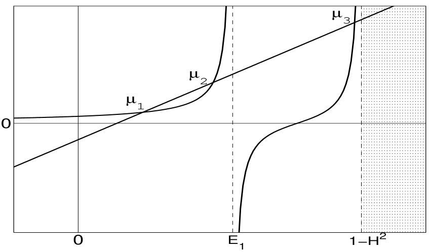
Figure 1: The graphical solution of the characteristic equation (78). The solid straight line depicts the function $y(\mu)=\mu-8H\Omega$ and the two solid curves intersecting it are branches of $y={\mathfrak{g}}(\mu)$.

Before discussing the roots, we would like to note that the characteristic equation (78) does not contain $\gamma$ explicitly. Having solved it for $\mu$ we can recover $\omega$ for any $\gamma$: $\omega=\sqrt{\mu-\gamma^{2}}$. This invariance of the eigenvalue problem in the space of scattering data is an exact equivalent of the invariance of the linearised eigenvalue problem in the space of solutions to the NLS equation [13].

The graph Fig.1 shows that the function $y={\mathfrak{g}}(\mu)$ and the straight line $y=\mu-8H\Omega$ have at least three intersections, $\mu_{1}$, $\mu_{2}$ and $\mu_{3}$ such that $\mu_{1}\leq\mu_{2}<E_{1}<\mu_{3}$. As $H$ grows, the straight line is shifted down and the function ${\mathfrak{g}}(\mu,H)$ also changes. In particular, for small $H$ the coefficients $\kappa^{2}$ increase in proportion to $H^{2}$ while the eigenvalue $E_{1}$ decreases and the edge of the continuous spectrum, $1-H^{2}$, also moves to the left. Hence for any fixed $\mu<E_{1}$ the corresponding ${\mathfrak{g}}(\mu)$ grows. As a result, the intersection points $\mu_{1}$ and $\mu_{2}$ approach each other, then merge for some critical value $H=H_{\rm cr}$ and emerge into the complex plane. As $H$ is increased past $H_{\rm cr}$, the imaginary parts of $\mu_{2}=\mu_{1}^{*}$ grow and eventually the positive imaginary part becomes equal to $\gamma$. This is the point of the Hopf bifurcation; for $H$ above this point the soliton (49) is unstable.

Conclusions of the above graphical analysis are in exact agreement with the behaviour of eigenvalues of the linearisation of equation (47) observed numerically [13]. A new feature is the appearance of another discrete eigenvalue, $\mu_{3}$, which was not detected in the numerical computations of [13, 18]. One reason for this omission could be that the separation of $\mu_{3}$ from the continuum remains exponentially small for small $H$. Indeed, for $H\to 0$ equation (77) infers that $\kappa(E_{1})=4\pi H^{3/2}+O(H^{5/2})$ and $\kappa(1-H^{2})=\sqrt{8\pi}H+O(H^{2})$. Assuming $\mu_{3}=1-H^{2}-\delta\mu$, where $\delta\mu/H^{2}\to 0$ as $H\to 0$, equation (79) gives ${\mathfrak{g}}(\mu,H)=-8\pi H^{2}\ln\delta\mu-2\pi^{2}H+O(H^{2})$. Substituting into (78), we obtain for the separation $\delta\mu$:

$$\delta\mu=\exp\left\{-\frac{1}{8\pi}\frac{1}{H^{2}}-\frac{2\pi^{2}-8}{8\pi}\frac{1}{H}+C\right\}\quad\mbox{as}\ H\to 0,$$ (80)

where $C=C(H)$ remains bounded as $H\to 0$. As $H$ grows, the frequency $\mu_{3}$ remains real and therefore does not give rise to any instabilities of the stationary solitons. However it may play a role in the resonance phenomena involving oscillating solitons.

We conclude this section with two remarks. First, our linearisation in the space of scattering data allows to explain the origin of the oscillatory instability of the soliton. When $H$ is very small, the soliton oscillations are virtually uncoupled from the radiation waves. The former have their frequency close to $\mu=0$ while the radiations have continuum of frequencies occupying the semiaxis $\mu\geq 1$. As $H$ is increased, the coupling grows, and as a result of that the soliton’s frequency is dragged closer to the continuum while another local mode is pulled out of the radiation spectrum. Finally, the two modes merge and the resonance occurs.

Second, we observe that as $k$ grows, the right-hand side of the bottom equation in (66) decreases rapidly. We also notice that only $\beta(k)$ with small $k$ contribute significantly to the right-hand side of the top equation. Consequently, only long radiation waves couple to the soliton. In the next section we study the effect of the $k=0$ radiation on the soliton’s nonlinear dynamics.

5 The long-wavelength limit

In order to study the soliton-radiation interaction at the long-wavelength limit, we write the spectral density $b(k)$ in the form $b({k})=b_{\epsilon}(k)=\epsilon^{-1}\tilde{b}({k}/\epsilon)$, where $\tilde{b}$ is an even function of its argument; integrate equations (63) and (64) over a small range of $k\in[-\delta k,\delta k]$ and then send $\epsilon\to 0$ in (61)-(64). This allows to derive a finite-dimensional system without any ad-hoc cut-off parameters (cf. [33, 38, 34]). The resulting four-dimensional system comprises equations for the amplitude and phase of the soliton, and the complex amplitude of the ${k}=0$ radiation:

$${\rho}+i{{\sigma}}=\lim_{\epsilon\to 0}\int\limits_{-\delta k}^{\delta k}{\rm d}{k}\,b_{\epsilon}({k}).$$

Skipping some lengthy but elementary calculations, we produce only the final result:

$$\dot{\Phi}=2(1-h\cos\Phi)-w,$$ (81)

$$\dot{w}=-\Bigl{\{}(\gamma+h\sin{\Phi})(4-\rho)-2{{\sigma}}h\cos{\Phi}\Bigr{\}}w,$$ (82)

$${\dot{\rho}}=\left\{\frac{w}{2}-{{\mathfrak{c}}}H+({{\mathfrak{c}}}+2)h\cos{\Phi}\right\}{{\sigma}}-(\gamma+h\sin{\Phi})(4-{\rho}),$$ (83)

$${\dot{\sigma}}=\left(-\frac{w}{2}+\frac{H}{3}+\frac{1}{3}h\cos{\Phi}\right){\rho}+(\gamma+3h\sin{\Phi}){{\sigma}}.$$ (84)

Here $w=8\eta^{2}$ and ${{\mathfrak{c}}}=4\ln 2-2\approx 0.77$.

Below we will compare conclusions based on the analysis of the four-dimensional system (81)-(84) with solutions of the full nonreduced NLS equation. To facilitate the comparison with results available in literature, we take the damped-driven NLS in autonomous form:

$$i\psi_{t}+\psi_{xx}+2|\psi|^{2}\psi=(1-i\gamma)\psi+h{\psi}^{*}.$$ (85)

Here $\psi$ is related to a solution of equation (47) by a simple phase transformation: $\psi(x,t)=-\exp(-i\Omega t)u(x,t)$. The value of the field (which is a sum of the soliton and radiation) at the centre of the soliton, i.e., at $x=0$, can be expressed through the variables of the reduced system. Using (51) and (59) we obtain in the limit $\epsilon\rightarrow 0$:

$$\left.\phantom{\frac{1}{1}}u(x,t)\right|_{x=0}=2i\eta\exp\left(i\Omega t-\frac{i}{2}\Phi\right)\left(1+\frac{i{{\sigma}}-{\rho}}{2\pi}\right),$$

and hence the value of the solution of the NLS (85) at the point $x=0$ is given by

$$\left.\phantom{\frac{1}{1}}\psi(x,t)\right|_{x=0}=\exp\left\{-i\left(\frac{\Phi+\pi}{2}\right)\right\}\sqrt{\frac{w}{2}}\left(1+\frac{i{{\sigma}}-{\rho}}{2\pi}\right)\equiv\psi_{0}(t).$$ (86)

The finite-dimensional system has two exact solutions. One of these,

$$\Phi=-\pi+\arcsin(\gamma/h),\quad w=2(1+H),\quad{\rho}={{\sigma}}=0,$$ (87)

corresponds to the pure-soliton solution of equation (85). The second solution arises by letting $w=0$, with $\Phi$ determined from the equation (81), and $\rho$ and $\sigma$ defined by the linear system (83) - (84). Choosing the constant of integration so that $\Phi(0)=0$, we obtain

$$\Phi(t)=2\arctan\left\{\left(\frac{1-h}{1+h}\right)^{\frac{1}{2}}\tan(\sqrt{1-h^{2}}\,t)\right\}\;{\rm mod\;}(2\pi).$$ (88)

Substituting this into equations (83) and (84), the system for ${\rho}$ and ${{\sigma}}$ becomes

$$\dot{\rho}=(\gamma+hd_{1})({\rho}-4)+(4\ln 2\,hd_{2}-{\mathfrak{c}}){{\sigma}},$$

(89)

$$\dot{\sigma}=(\gamma+3hd_{1}){{\sigma}}+\frac{1}{3}(H-hd_{2}){\rho},$$

where

$$d_{1}=\sin\Phi(t)=\frac{\sqrt{1-h^{2}}\sin(2\sqrt{1-h^{2}}t)}{1+h\cos(2\sqrt{1-h^{2}}t)},\quad d_{2}=\cos\Phi(t)=\frac{h+\cos(2\sqrt{1-h^{2}}t)}{1+h\cos(2\sqrt{1-h^{2}}t)}.$$

In view of equations (52) and (59), $w=0$ amounts to $\psi(x,t)=u(x,t)=0$ and hence the above $w=0$ solution corresponds to the flat zero solution of the full nonreduced NLS equation (85). This fact is quite remarkable. Indeed, although the system (81)-(84) was derived under the assumption of the proximity to the (damped driven) soliton, it does possess the flat solution which cannot be regarded as the soliton’s small perturbation. As in the full partial differential equation (85), where the unstable soliton can decay to the flat attractor, finite-dimensional trajectories starting near the unstable fixed point (87) can be attracted to the $w=0$ solution. An example of such evolution, obtained numerically, is presented in Fig. 2, for $t\in[0,250]$.

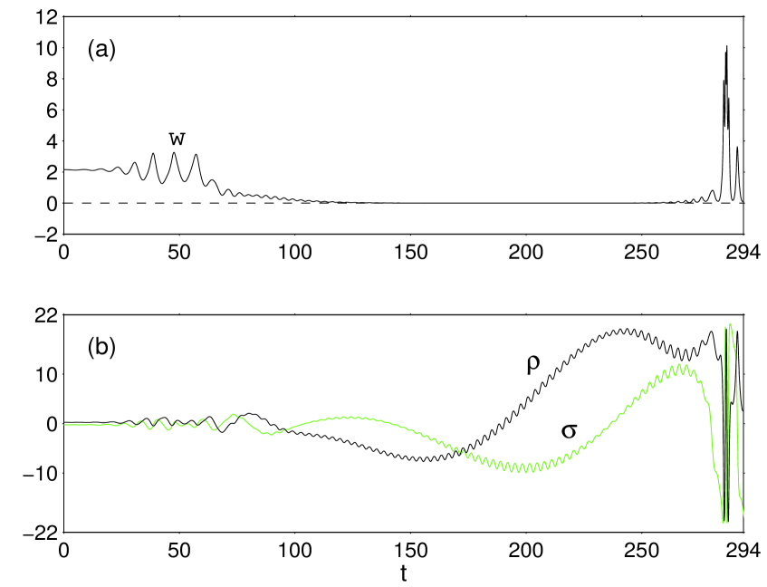
Figure 2: A numerical evolution of $w$, $\rho$, and $\sigma$: an attraction to the $w=0$ solution and an explosive instability of the latter due to the exponential growth of $\rho$ and $\sigma$.

It is important to note here that for $\gamma>0$, solutions to the linear system (89) are exponentially growing functions (see Fig. 2(b)). This is not in disagreement with the fact that the corresponding $\psi(x,t)$ is zero for all $x$ and $t$. Indeed, the total amplitude of the long-wavelength radiation includes a factor $\eta$ (see e.g. (59) or (86).) Therefore, if $w=\eta=0$, the total amplitude is zero no matter what ${\rho}$ and ${{\sigma}}$ are equal to.

The fact that $\rho$ and $\sigma$ are exponentially growing functions, gives rise to an instability of the $w=0$ solution of the system (81)-(84). Indeed, the multiplier

$${\mathfrak{r}}(t)=-\left\{(\gamma+h\sin\Phi)(4-\rho)-2\sigma h\cos\Phi\right\}$$

in the right-hand side of (82), may assume large positive values. (For example, each time $\sin\Phi$ goes through 1, ${\mathfrak{r}}(t)$ becomes equal to approximately $(\gamma+h)\rho$.) This means that for $w\,^{<}\!\!\,\!\!_{\sim}\,1$ we have two different time scales in the system: the variables $\Phi$, $\rho$ and $\sigma$ do not change appreciably on intervals $\Delta t\,^{<}\!\!\,\!\!_{\sim}\,1$ and can be considered constant, while $w$ grows with the exponential growth rate ${\mathfrak{r}}\gg 1$. Consequently, if $w$ is assigned a small but nonzero value at the moment of time when ${\mathfrak{r}}(t)$ is large, it will quickly (within $\Delta t\sim{\mathfrak{r}}^{-1}$) grow to values of order ${\mathfrak{r}}$. This is indeed observed in simulations, see Fig.2 for $t>250$. However, the instability of the $w=0$ solution is spurious — in the sense that it does not mirror any genuine instabilities of the zero solution in the full NLS equation.

6 Reduced finite-dimensional dynamics

6.1 Onset of instability

Linearising the system (81)-(84) about the fixed point (87) and using (46), we obtain

$${\ddot{\phi}}+2\gamma{\dot{\phi}}+8H(1+H){\phi}=4H(1+H){{\sigma}},$$ (90)

$${\ddot{\sigma}}+2\gamma{\dot{\sigma}}+(1+H)[1-(2{\mathfrak{c}}+1)H]{\sigma}=-4H(1+H){\phi}.$$ (91)

Here $\phi$ is the perturbation of the soliton’s phase, defined as $\phi=\Phi-\Phi_{+}$. Letting ${\phi}(t)=\chi e^{\lambda t}$ and ${{\sigma}}(t)={{\sigma}}_{0}e^{\lambda t}$, where $\lambda=-\gamma+i\omega$, we obtain the characteristic equation for complex $\omega$:

$${\omega}^{4}-(\Omega_{s}^{2}+\Omega_{r}^{2}-2\gamma^{2}){\omega}^{2}+(\Omega_{s}^{2}-\gamma^{2})(\Omega_{r}^{2}-\gamma^{2})+16H^{2}(1+H)^{2}=0.$$ (92)

Here

$$\Omega_{s}^{2}=8H(1+H),\quad\Omega_{r}^{2}=(1+H)[1-(2{{\mathfrak{c}}}+1)H].$$

Like the eigenvalue problem (74)-(76) for the full set of spectral data (and like the eigenvalue problem for the underlying partial differential equation [13]), the characteristic equation (92) can be conveniently reformulated in terms of the self-similar variable $\mu=\gamma^{2}+\omega^{2}$:

$${\mu}^{2}-p\mu+q=0,$$ (93)

where

$$p=p(H)=\Omega_{s}^{2}+\Omega_{r}^{2},\quad q=q(H)=\Omega_{s}^{2}\Omega_{r}^{2}+16H^{2}(1+H)^{2}.$$

The fact that the reduced system (81)-(84) inherits the self-similarity of the parent PDE, deserves to be specially emphasised. It implies that the reduction procedure based on the Riemann-Hilbert problem — unlike the variational reductions [42, 43] — preserves the structure of the infinite-dimensional phase space.

The fixed point is unstable when ${\rm Re\/}\lambda>0$. In terms of $\mu$, this condition translates into

$$\frac{[{\rm Im\/}\mu(H)]^{2}}{4{\rm Re\/}\mu(H)}\geq\gamma^{2}.$$ (94)

The discriminant of (93) is

$$D(H)=(H_{1}H_{2})^{-1}(1+H)^{2}(H-H_{1})(H-H_{2}),$$

where $H_{1}=(8\ln 2+13)^{-1}\approx 0.054$ and $H_{2}=(8\ln 2-3)^{-1}\approx 0.39$. Between $H_{1}$ and $H_{2}$ the quadratic (93) has a pair of complex-conjugate roots while outside this interval both roots are real and nonnegative (Fig. 3). Consequently, the inequality (94) can only hold for $H_{1}\leq H\leq H_{2}$. For $H$ within this interval the inequality (94) amounts to

$$8\gamma^{2}\leq-D(H)/p(H).$$ (95)

For small $\gamma$ the cubic equation $D(H)/p(H)=-8\gamma^{2}$ has one negative and two positive roots which we denote ${\cal H}_{1}(\gamma)$ and ${\cal H}_{2}(\gamma)$, $0<{\cal H}_{1}(\gamma)<{\cal H}_{2}(\gamma)$. (Note that ${\cal H}_{1}(0)=H_{1}$ and ${\cal H}_{2}(0)=H_{2}$; hence the notation.) Recalling that $H=\sqrt{h^{2}-\gamma^{2}}$, the instability inequality (95) can be rewritten as

$$\sqrt{{\cal H}_{1}^{2}(\gamma)+\gamma^{2}}\leq h\leq\sqrt{{\cal H}_{2}^{2}(\gamma)+\gamma^{2}}.$$ (96)

As $\gamma$ is increased, the positive roots ${\cal H}_{1}(\gamma)$ and ${\cal H}_{2}(\gamma)$ merge and become complex. For greater $\gamma$ the inequality (94)-(95) cannot be satisfied by any $h$.

Equation (96) gives an explicit form of the instability region on the $(h,\gamma)$-plane (Fig.4). As $h$ is increased past the value $h=\sqrt{{\cal H}_{1}^{2}+\gamma^{2}}$ (or decreased below $h=\sqrt{{\cal H}_{2}^{2}+\gamma^{2}}$), the fixed point becomes unstable via a Hopf bifurcation.

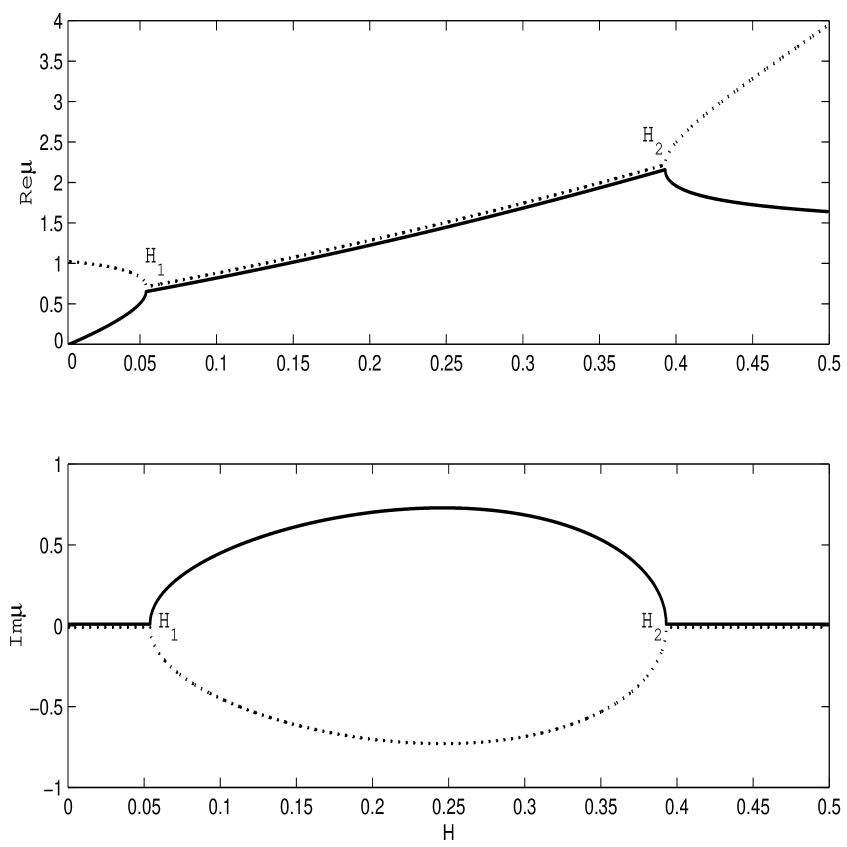
Figure 3: The real (a) and imaginary (b) parts of the roots to the characteristic equation (93).

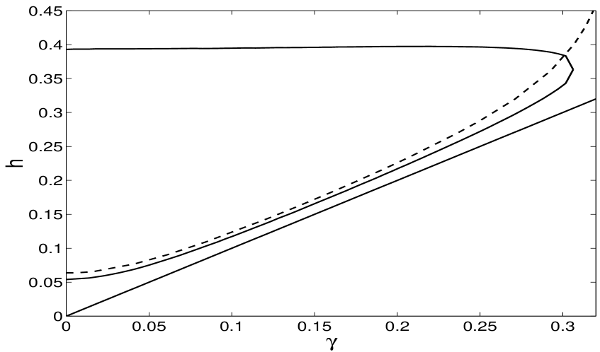
Figure 4: Solid curve: the boundary of the instability region of the fixed point. (The fixed point is unstable inside the “parabola”.) Dashed curve: the line of the Hopf bifurcation of the stationary soliton of the full NLS equation (85). (The soliton is unstable above the dashed curve.) Also shown is the straight line $h=\gamma$, the boundary of the existence domain of both the soliton and the fixed point (87).

The instability setting in for $H>{\cal H}_{1}(\gamma)$ corresponds to the Hopf instability of the soliton in the full damped-driven NLS equation. Note however that the finite-dimensional instability threshold $h=\sqrt{{\cal H}_{1}^{2}(\gamma)+\gamma^{2}}$ is somewhat lower than the instability threshold in the partial differential equation (which is also shown in Fig. 4). On the other hand, the upper boundary of the instability region, $h=\sqrt{{\cal H}_{2}^{2}(\gamma)+\gamma^{2}}$, does not have a counterpart in the full NLS equation. (In the full PDE, the soliton does not restabilise as $h$ is increased [13].) This fact alone is sufficient to conclude that the finite-dimensional system cannot be expected to provide a good approximation to the infinite-dimensional dynamics for $h$ greater than approximately $0.4$.

In order to find attractors in the region inside the parabola (96), where the fixed point is unstable, we performed a series of numerical simulations of equations (81)-(84). Here our strategy was similar to that used in the simulations of the full nonreduced NLS equation [17]; that is, we varied $h$ for a fixed value of $\gamma$. We also adopted the same strategy with regard to the choice of the initial conditions. Our simulations always started with the (unstable) fixed point perturbed by values of order $10^{-14}$ which is several orders of magnitude smaller than the local discretisation error of the Runge-Kutta approximation. (For some values of $h$ and $\gamma$ the final state of the system was extremely sensitive to tiny changes of this perturbation.)

6.2 Finite-dimensional attractors; $\gamma\neq 0$

As $h$ is increased for a fixed nonzero $\gamma$ (with $\gamma\leq 0.31$), a limit cycle is born supercritically at the point of the Hopf bifurcation, $h=\sqrt{{\cal H}_{1}^{2}(\gamma)+\gamma^{2}}$. This is in exact agreement with the full partial differential equation. The subsequent bifurcation diagram depends on the value of $\gamma$.

For $\gamma$ greater than approximately 0.2, the stable limit cycle persists as $h$ is increased all the way up to $h=\sqrt{{\cal H}_{2}^{2}(\gamma)+\gamma^{2}}$ where it shrinks back to the fixed point. On the contrary, if we increase $h$ for a smaller $\gamma$, $0.12<\gamma\leq 0.20$, the limit cycle looses its stability at a certain value $h=h_{\rm z}$ (where $h_{\rm z}<\sqrt{{\cal H}_{2}^{2}+\gamma^{2}}$.) For $h$ above $h_{\rm z}$, the finite-dimensional trajectory emanating from any initial condition, quickly settles to the $w=0$ solution corresponding to the zero attractor of the full nonreduced NLS. (This is illustrated by Fig.2 and, for a different $\gamma$, Fig.5(b).) Increasing $h$ still further, the $w=0$ solution persists as the only attractor over a sizeable range of $h$ values — until a stable limit cycle reappears. This range becomes wider for smaller values of $\gamma$.

The range of driving strengths where the only attractor is $w=0$, exists for all $\gamma\in(0,0.20]$ (although for some $\gamma$ the limit cycle may undergo a number of intermediate bifurcations before disappearing from the attractor chart; see below.) This is in exact agreement with the behaviour observed in the full partial differential equation [17] where the solitonic attractor undergoes a crisis and the flat zero solution remains the only attractor in the system. Thus we may conclude that taking into account the coupling of the soliton to the $k=0$ radiation, is sufficient to explain the occurrence of the “desert region” on the $(h,\gamma)$-plane. It is appropriate to mention here that a similar “desert” spanned just by a flat attractor, arises in the externally driven NLS [33, 38]. It is natural to assume that the appearance of the “flat desert” in the latter system can be still explained by the soliton-longwave radiation coupling. (The failure of the four-dimensional reduced systems proposed in [33, 38, 34] to capture the crisis of the localised attractor and reproduce the “desert”, should be probably attributed to nonoptimal variational Ansätze.)

Although our finite-dimensional system with $\gamma\leq 0.2$ correctly reproduces the sequence of attractors arising in the full PDE (stationary soliton $\to$ oscillating soliton $\to$ zero solution), it does not necessarily capture fine details of this sequence. Unlike the oscillating soliton in the full NLS equation, for $\gamma$ between 0.12 and 0.20 the finite-dimensional limit cycle does not undergo any period-doubling bifurcations. The largest $\gamma$ for which the period-doubling occurs in the reduced system (81)-(84), is $\gamma=0.12$. In this case the period-2 cycle arises at $h=0.16$ and then degenerates back to the period-1 as $h$ is increased past $h=0.17$. Increasing $h$ still further, the period-1 yields to the $w=0$ solution for $h\geq 0.195$, without any intermediate period-doublings. A similar pattern arises for $\gamma=0.11$.

In the case $\gamma=0.10$ the sequence of finite-dimensional attractors is richer. In this case we observed the whole cascade of period-doubling bifurcations, culminating, for $h=0.146$, in a chaotic attractor (centred on the fixed point). For $h$ between 0.146 and 0.150 the only attractor was found to be $w=0$; for $h=0.150$ the chaotic attractor reappears, and for even greater $h$ it degenerates to the period-2 (for $h=0.165$) and then period-1 cycle (for $h=0.170$). At $h=0.18$ the cycle disappears and $w=0$ was the only attractor we detected in a wide band of $h$ values above $h=0.18$. Next, increasing $h$ for the fixed $\gamma=0.05$ and 0.07, the period-1 ($P1$) limit cycle yields to the period-2 ($P2$) and then to $w=0$. For $\gamma=0.06$ the sequence of attractors was $P1\to$ $P2\to$ $(w=0)\to$ $P3\to$ $P4\to$ (a 4-band chaotic attractor) $\to$ $(w=0)\to$ (a 2-band chaos coexisting with $P3)\to$ (a 1-band chaos) $\to$ $(w=0)$. (The last two regimes are illustrated in Fig.5.) The full NLS equation also exhibits a rich host of attractors for $\gamma>0.05$, including the chaotic soliton [17], [39]; however, details of the two bifurcation diagrams do not necessarily coincide.

It is only for very small $\gamma$ that the finite- and infinite-dimensional dynamics are in exact agreement. Increasing $h$ for the fixed $\gamma=0.01,0.02$ and 0.04, the period-1 cycle yields directly to the $w=0$ attractor. This is consistent with the absence of the period-doubling in the full PDE. The smallest $\gamma$ for which the period-2 soliton was observed there, was $\gamma=0.055$ [39].

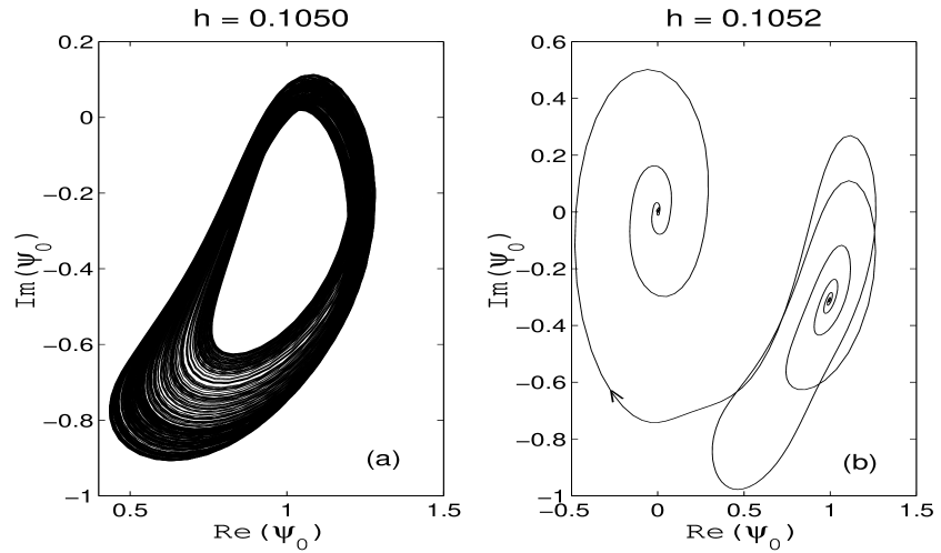
Figure 5: Trajectories in the four-dimensional system (81)-(84) with $\gamma=0.06$. (a) A strange attractor corresponding to the chaotic soliton. (b) A crisis of the chaotic attractor: the trajectory escapes from the neighbourhood of the fixed point and flows into the $w=0$ solution. To facilitate the comparison with the corresponding regimes in the PDE, the trajectories are presented in terms of the real and imaginary parts of the quantity (86).

6.3 The undamped case, $\gamma=0$

This case deserves a separate consideration as the arising attractors are very different from those occurring for nonzero damping. Consistently with the PDE [18], no limit cycles were detected for $\gamma=0$. Instead, we observed two types of chaotic regimes. For $h$ in a narrow interval $0.0539<h<0.06$ just above the Hopf bifurcation value $h=H_{1}=0.0539$, the trajectory was seen to wind chaotically in an annulus centred on the unstable fixed point (Fig.6a). The outer radius of the annulus is approximately one order of magnitude smaller than $w=2(1+h)$, the $w$-coordinate of the fixed point. This proximity of the orbit to the fixed point justifies one of the assumptions made in the derivation of the finite-dimensional system (81)-(84). The strange attractor shown in Fig.6a represents small chaotic oscillations of the amplitude of the soliton about its stationary value $\left|\psi\right|_{x=0}=\sqrt{1+h}$. The chaotic oscillations of the undamped soliton were indeed observed in numerical simulations of the full nonreduced NLS equation [40]; however these would die out as transients and the evolution settle to either a slowly growing or decaying breather [18]. The fact that the chaotic attractor does not arise in the full partial differential equation with $\gamma=0$ and only persists as a transient chaos, can be explained by the interaction of the soliton with short and medium wavelength radiations — which we have neglected in our present derivation of the finite-dimensional system. For $h$ greater than 0.06 (but smaller than $H_{2}=0.39$, the upper boundary of the fixed point’s instability domain), the chaotic solution is no longer centred on the fixed point. (See Fig.6b). What is even more important, the amplitude of the aperiodic oscillations grows rapidly. Therefore the finite-dimensional system is not applicable in this region and the chaotic solution shown in Fig.6b does not have a counterpart in the full nonreduced partial differential equation.

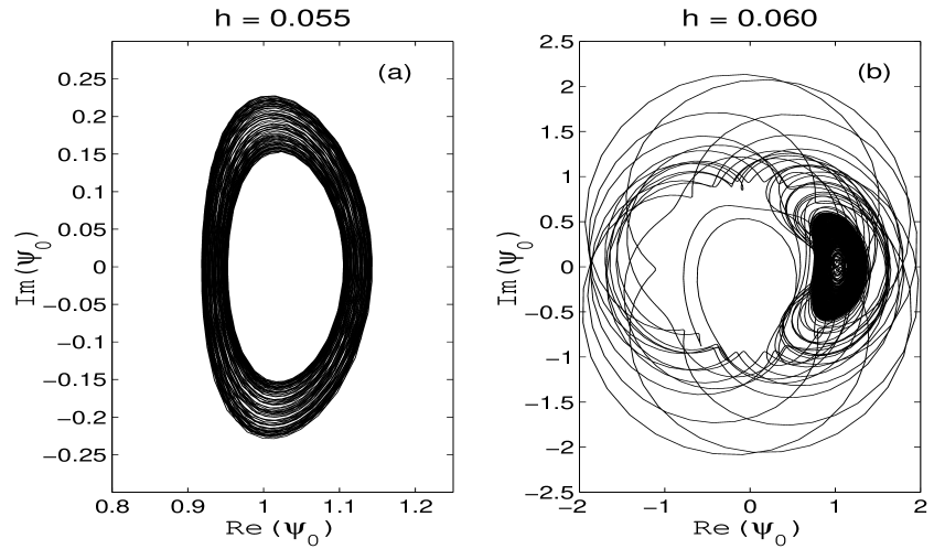
Figure 6: Trajectories in the finite-dimensional system (81)-(84) with $\gamma=0$. The strange attractor (a) and its crisis (b).

7 Conclusions

It was proposed by various authors [18, 33, 34, 35, 41] that the coupling to the radiation (more specifically, to its long-wavelength component [33, 34, 35, 38]) is the key factor determining the internal dynamics of the damped driven soliton, in particular its instability, bifurcations and transition to chaos. The main objective of the present work was to study the role of the soliton-radiation interaction within an approach which allows a rigorous decomposition of the phase space into the soliton and radiation modes. Our treatment is based on the Riemann-Hilbert problem, a modern version of the Inverse Scattering transform. Although the Inverse Scattering method had already been utilised in a related context (for the externally driven NLS [26, 33, 34, 41]), our approach is different in that we are not assuming the damping and driving terms to be small in any sense. Instead, we are exploiting a remarkable coincidence between the mathematical formula for the parametrically driven damped soliton and that of the soliton of the unperturbed NLS. This coincidence allows to associate the stationary damped-driven soliton with a stationary zero of the Riemann-Hilbert problem — for any $h$ and $\gamma$. The evolution of all nearby solutions $\psi(x,t)$ can therefore be studied through the evolution of the corresponding scattering data.

Some interesting insights are gained already from the linearised equations for the spectral data. Conclusions of this analysis are consistent with results of the linearisation in the space of fields $\psi(x,t)$ [13]; however the linearisation in the spectral space has an important advantage that it can be carried out analytically whereas linearised equations for $\psi(x,t)$ could only be studied by means of computer. The stationary soliton looses its stability as a result of its coupling to radiation waves. This had already been proposed before [42] but now we have put this claim on rigorous footing.

We attempted to advance beyond the linear approximation and track the effect of the long-wavelength radiation on the nonlinear dynamics of the soliton. To find a closed system for the evolution of the scattering data, we had to make two assumptions. First, we assumed that the solution of our damped driven NLS remains close to the stationary soliton of the same, perturbed, equation. Second, we assumed that the resulting system for the evolution of the spectral data is linear in radiation. (Note that we are not requiring the perturbation in the right-hand side of (1) to be small in any sense.)

The outcome of this analysis is a dynamical system (81)-(84) comprising equations for the amplitude and phase of the soliton, and for the complex amplitude of the $k=0$-radiation. Finite-dimensional reductions of both externally [33, 34, 35, 38] and parametrically [42, 43] driven NLS are available in literature and hence we need to emphasise the differences. The principal difference between our reduction and those obtained variationally [34, 38, 42, 43] or by the Galerkin projections [35], lies in that our system of ODEs is not a product of any phenomenological Ansatz. It results from a rigorous expansion of the solution of the PDE over a set of “nonlinear modes” and then retaining only those modes whose effect on the dynamics we are trying to track down. A failure of one or the other variational or Galerkin approximation to capture essentials of the supercritical dynamics of the soliton does not provide any information on why this particular Ansatz fails. One has to try a variety of different Ansätze, select the one that gives the best fit and then attempt to make some semi-intuitive conclusions on the role of this or that ingredient of the trial function. On the contrary, our approach allows to explore, systematically, each part of the phase space and identify the nonlinear modes responsible for each particular dynamical effect. Next, our reduction technique is different from the approach of an influential paper [33] which is also partially based on the Inverse Scattering. Besides the fact that the analysis of Ref. [33] relies on the smallness of the perturbation, it only uses the Inverse Scattering transform to obtain the functional form of the radiation wave whereas its interaction with the soliton is introduced variationally. The damping term for the radiation was not part of the variational algorithm and had to be added in an ad-hoc way. The method does not define the amplitude of the radiation either; this is introduced empirically and then fitted to match the numerical data. Unlike Ref. [33], our finite-dimensional reduction is uniquely defined by the choice of the ingredients of the localised attractor and does not require introduction of any phenomenological terms or fitting parameters. This uniqueness is reflected by the fact that (the linearisation of) our reduced system retains the self-similarity invariance of the (linearised) PDE.

The analysis of the reduced dynamical system shows that it is capable of explaining only some parts and only some rough features of the attractor chart of the parametrically driven damped NLS [17]. Most notably, the interaction with long radiation waves is sufficient to reproduce the approximate sequence of attractors arising when the driving strength is increased under the fixed dissipation coefficient. Consistently with computer simulations of [17, 39], the finite-dimensional system exhibits the sequence “stationary soliton $\to$ periodically oscillating soliton” for larger dampings and “stationary soliton $\to$ oscillating soliton $\to$ flat zero solution” for smaller $\gamma$. For $\gamma=0$ the reduced system does not predict oscillating solitons with bounded amplitudes (apart from a tiny window of $h$ values). This is also in agreement with the behaviour observed in the full PDE [18]. However, the finite-dimensional system predicts — erroneously — the occurrence of the second, restabilising, Hopf bifurcation. As a result of that, the finite-dimensional fixed point turns out to be stable for all $\gamma$ as long as $h\geq 0.4$, whereas the actual stability domain of the stationary soliton is much smaller [13]. One could have expected that the reduced and infinite-dimensional dynamics would be close in the region adjacent to the first, destabilising, Hopf bifurcation curve — which does provide a reasonably good approximation to the Hopf bifurcation curve in the full PDE. In the actual fact, however, details of the attractors and bifurcation sequences in the two systems are quite different even in that region. (An exception is the band of very small $\gamma$, $\gamma<0.05$.)

Thus, taking into account just the $k=0$ component of radiation is insufficient for reproducing the entire complexity in the damped-driven soliton’s dynamics. It is quite possible that the radiation waves with the frequency close to the double frequency of the soliton’s linear oscillations [18] play a more important (or equally important) role than those with $k=0$. On the other hand, numerical simulations on finite intervals reveal the excitation of radiations with several wavenumbers [41]. It is not unprobable that a similar wavenumber selection and competition occur on the infinite line. Finally, there are indications that the oscillating soliton of the externally driven NLS, is in fact a bound state of two solitons of the unperturbed, integrable, NLS equation [38]. A similar mechanism may operate in the parametrically driven case as well. Our approach allows to test all these possibilities; we are planning to do so in future publications.

8 Acknowledgements

We are grateful to Nora Alexeeva for her help in the course of this work. This project was supported by grants from the Research Council of the University of Cape Town and the National Research Foundation of South Africa.

9 Appendix: Discrete eigenvalues of the operator ${\hat{\cal G}}$

Here we demonstrate the existence of, and derive a lower bound for, discrete eigenvalues of the operator ${\hat{\cal G}}$, equation (67). The smallest eigenvalue, $E_{1}$, can be sought for as a minimum of the corresponding Rayleigh quotient:

$$E_{1}=\min_{\psi(k)}\frac{\int{\rm d}{k}\psi{\hat{\cal G}}\psi}{\int{\rm d}{k}\psi^{2}}.$$ (97)

In terms of $\varphi=(1+{k}^{2})\psi$, this can be rewritten as

$$E_{1}=\min_{\varphi(k)}\frac{\int{\rm d}{k}\varphi\left\{(1+{k}^{2})^{-2}\left[(1+\Omega{k}^{2})^{2}-H^{2}\right]+2H\Omega{\hat{\cal F}}\right\}\varphi}{\int{\rm d}{k}(1+{k}^{2})^{-2}\varphi^{2}},$$ (98)

where we have introduced a symmetric operator ${\hat{\cal F}}$:

$${\hat{\cal F}}\varphi({k})=(1+{k}^{2})^{-1}{\hat{\cal B}}(1+{k}^{2})^{-1}\varphi({k}).$$ (99)

(Here ${\hat{\cal B}}$ is given by (68).)

For $H=0$ the operator ${\hat{\cal G}}$ does not have discrete eigenvalues but as $H$ grows, at least one discrete eigenvalue detaches from the continuum. Indeed, in the region $|\ell|<1$, $|{k}|<1$ the kernel of the operator ${\hat{\cal F}}$,

$${\cal F}(\ell,{k})=\frac{({{k}}-{\ell})({\ell}{{k}}-1)}{\sinh\left[\frac{\pi}{2}({{k}}-{\ell})\right]}\frac{1}{(1+{{k}}^{2})^{3/2}(1+{\ell}^{2})^{3/2}},$$

satisfies

$${\cal F}(\ell,k)\leq\frac{1}{4\sinh\pi}(\ell k-1).$$ (100)

For an arbitrary even function $h(k)$ the inequality (100) yields

$$\int\limits_{-1}^{1}\int\limits_{-1}^{1}{\rm d}k{\rm d}\ell\,h(k){\cal F}(k,\ell)h(\ell)<-\frac{1}{4\sinh{\pi}}\left(\,\int\limits_{-1}^{1}{\rm d}kh(k)\right)^{2}.$$ (101)

Choosing a suitable trial function $\psi=\psi_{H}(k)$ in the quotient (97) and using the estimate (101), one readily concludes that for any positive $H$ the quotient can take values lying below $1-H^{2}$, the edge of the continuous spectrum. Hence the operator ${\hat{\cal G}}$ has at least one discrete eigenvalue for $H>0$.

Next, the norm of the operator (99) is bounded:

$$||{\hat{\cal F}}||^{2}=\int\limits_{-\infty}^{\infty}\int\limits_{-\infty}^{\infty}{{\rm d}}{{k}}{{\rm d}}{\ell}\,{\cal F}^{2}(\ell,{k})<\frac{5}{8}.$$

Therefore ${\hat{\cal F}}$ is a Fredholm operator and its eigenvalues ${\cal E}_{m}$, ${\hat{\cal F}}\phi_{m}={\cal E}_{m}\phi_{m}$, are bounded:

$${\cal E}_{m}^{2}<||{\hat{\cal F}}||^{2}<\frac{5}{8}.$$ (102)

Returning to the operator ${\hat{\cal G}}$ (67), its eigenvalue $E_{n}$ $(n=1,2,...)$ satisfies

$$E_{n}=\frac{\int{\rm d}{k}\psi_{n}{\hat{\cal G}}\psi_{n}}{\int{\rm d}{k}\psi_{n}^{2}},$$ (103)

where $\psi_{n}(k)$ is the associated eigenfunction: ${\hat{\cal G}}\psi_{n}=E_{n}\psi_{n}$. Using inequality (102) in equation (103) we obtain a lower bound on $E_{n}$:

$$E_{n}>\frac{\int{\rm d}{k}\varphi_{n}\left(1-H^{2}+2H\Omega{\hat{\cal F}}\right)\varphi_{n}}{\int{\rm d}{k}\varphi_{n}^{2}}>(1-H^{2})\left[1-\frac{H\Omega}{1-H^{2}}\sqrt{\frac{5}{2}}\,\right],$$ (104)

where $\varphi_{n}=(1+k^{2})\psi_{n}$.

References

-
[1]
Miles J W 1984 Nonlinear Faraday resonance J. Fluid.
Mech. 146 285;
1984 Parametrically excited solitary waves J. Fluid. Mech. 148 451 - [2] Elphick C and Meron E 1989 Localised structures in surface waves Phys. Rev. A 40 3226
- [3] Umeki M and Kambe T 1989 Nonlinear dynamics and chaos in parametrically excited surface waves J. Japan Soc. Fluid. Mech. 8 157
- [4] Kambe J and Umeki M 1990 Nonlinear dynamics of two-mode interactions in parametric excitation of surface waves J. Fluid. Mech. 212 373
- [5] Laedke E W and Spatschek K H 1991 On localized solutions in nonlinear Faraday resonance J. Fluid. Mech. 223 589
-
[6]
Umeki M 1991 Parametric
dissipative nonlinear Schrödinger equation J. Phys. Soc. Jpn.
60 146;
1991 Faraday resonance in rectangular geometry J Fluid Mech 227 161 - [7] Yan J R and Mei R J 1993 Interaction between two Wu’s solitons Europhys. Lett. 23 335
- [8] Chen X -N and R -J Wei R -J 1994 Dynamic behaviour of a non-propagating soliton under a periodically modulated oscillation J. Fluid. Mech. 259 291
-
[9]
Wang X and Wei R 1997
Interactions and motions of double-solitons with opposite polarity in a
parametrically driven system Phys. Lett. A 227 55;
1997 Dynamics of multisoliton interactions in parametrically resonant systems Phys. Rev. Lett. 78 2744;
1998 Oscillatory patterns composed of the parametrically excited surface-wave solitons Phys. Rev. E 57 2405 - [10] Il’ichev A 1998 Faraday resonance: Asymptotic theory of surface waves Physica D 119 327
- [11] Miao G and Wei R 1999 Parametrically excited hydrodynamic solitons Phys. Rev. E 59 4075
- [12] Astruc D and Fauve S 2001 Parametrically Amplified 2-Dimensional Solitary Waves In: IUTAM Symposium on Free Surface Flows. Proceedings of the IUTAM Symposium held in Birmingham, UK, 10-14 July 2000. A. C. King and Y. D. Shikhmurzaev, editors. Fluid mechanics and its applications, Vol. 62 (Kluwer, 2001).
- [13] Barashenkov I V, Bogdan M M and Korobov V I 1991 Stability diagram of the phase-locked solitons in the parametrically driven damped nonlinear Schrödinger equation Europhys. Lett. 15 113
- [14] Deutsch I H and Abram I 1994 Reduction of quantum noise in soliton propagation by phase-sensitive amplification J. Opt. Soc. Am. B 11 2303 1994
- [15] Mecozzi A, Kath L, Kumar P and Goedde C G 1994 Long-term storage of a soliton bit stream by use of phase sensitive amplification Opt. Lett. 19 2050
- [16] Longhi S 1995 Ultrashort-pulse generation in degenerate optical parametric oscillators Opt. Lett. 20 695
- [17] Bondila M, Barashenkov I V and Bogdan M M 1995 Topography of attractors of the parametrically driven nonlinear Schrödinger equation Physica D 87 314
- [18] Alexeeva N V, Barashenkov I V and Pelinovsky D E 1999 Dynamics of the parametrically driven NLS solitons beyond the onset of the oscillatory instability Nonlinearity 12 103
- [19] Zakharov V E and Shabat A B 1972 Exact theory of two-dimensional self-focusing and one-dimensional self-modulation of waves in nonlinear media Sov. Phys. JETP 34 62
- [20] Zakharov V E and Shabat A B 1979 Integration of nonlinear equations of mathematical physics by the method of the inverse scattering Funct. Anal. Appl. 13 13
- [21] Novikov S P, Manakov S V, Pitaevski L P and Zakharov V E 1984 Theory of Solitons. The Inverse Scattering Method (Consultants Bureau, New York)
- [22] Faddeev L D and Takhtajan L A 1987 Hamiltonian Methods in the Theory of Solitons (Springer-Verlag, Berlin-Heidelberg-New York)
- [23] Ablowitz M J and Clarkson P A 1991 Solitons, Nonlinear Evolution Equations and Inverse Scattering (Cambridge University Press, Cambridge)
-
[24]
Kaup D J 1976 A perturbation expansion for the
Zakharov-Shabat inverse scattering transform SIAM J. Appl. Math.
31 121;
1990 Perturbation theory for solitons in fibers Phys. Rev. A 42 5689 - [25] Karpman V I and Maslov E M 1977 Perturbation theory for solitons Sov. Phys. JETP 46 281
-
[26]
Kaup D J and Newell A C 1978 Solitons as particles,
oscillators and in slowly varying media: a singular perturbation theory
Proc. R. Soc. London Ser. A
361 413;
1978 Theory of nonlinear oscillating dipolar excitations in one-dimensional condensates Phys. Rev. B 18 5162 - [27] Kodama Y and Ablowitz M J 1981 Perturbations of solitons and solitary waves Stud. Appl. Math. 64 225
- [28] Maslov E M 1980 Second order perturbation theory for solitons Teor. Mat. Fiz. 42 362 [Theor. Math. Phys. 42 (1980) 237]
- [29] Kaup D J 1991 Second-order perturbations for solitons in optical fibers Phys. Rev. A 44 4582
- [30] Doktorov E V and Prokopenya I N 1991 On higher-order corrections in soliton perturbation theory Inverse Problems 7 221
- [31] Shchesnovich V S and Doktorov E V 1997 Perturbation theory for solitons of the Manakov system Phys. Rev. E 55 7626; 1999 Perturbation theory for the modified nonlinear Schrödinger solitons Physica D 129 115
- [32] Kivshar Yu S and Malomed B A 1989 Dynamics of solitons in nearly integrable systems Rev. Mod. Phys. 61 763
-
[33]
Nozaki K and Bekki N 1985 Chaotic solitons
in a plasma driven by an rf field J. Phys. Soc. Jpn.
54 2363;
1986 Low-dimensional chaos in a driven damped nonlinear Schrödinger equation Physica D 21 381 - [34] Taki M, Spatschek K H, Fernandez J C, Grauer R, Reinisch G 1989 Breather dynamics in the nonlinear Schrödinger regime of perturbed sine-Gordon systems Physica D 40 65
- [35] Grauer R and Birnir B 1992 The center manifold and bifurcations of damped and driven sine-Gordon breathers Physica D 56 165
- [36] Bogdan M M, Kosevich A M and Manzhos I V 1985 Stabilisation of a magnetic soliton (bion) as a result of parametric excitation of one-dimensional ferromagnet Fizika Nizkih Temperatur 11 991 [Sov. J. Low Temp. Phys. 11 547 (1985)]
- [37] Fauve S and Thual O 1990 Solitary waves generated by subcritical instabilities in dissipative systems Phys. Rev. Lett. 64 282
- [38] Spatschek K H, Pietsch H, Laedke E W and Eickermann Th 1989 On the role of soliton solutions in temporal chaos: examples for plasmas and related systems, in: Proceedings of the International Conference on Singular Behaviour and Nonlinear Dynamics, Samos, 1988. World Scientific, Singapore
- [39] Bondila M 1998 MSc thesis (University of Cape Town)
- [40] Alexeeva N V, private communication
- [41] Bishop A R, Forest M G, McLaughlin D W and Overman E A II 1986 A quasi-periodic route to chaos in a near-integrable PDE Physica D 23 293
- [42] Barashenkov I V, Bogdan M M and Korobov V I 1991 Stability properties of exact soliton solutions of the parametrically driven, damped nonlinear Schrödinger equation. In: Nonlinear Evolution Equations and Dynamical Systems. Research Reports in Physics. Editors: Makhankov V G and Pashaev O K. Springer-Verlag, Berlin
- [43] Longhi S, Steinmeyer G and Wong W S 1997 Variational approach to pulse propagation in parametrically amplified optical systems J. Opt. Soc. Am. B 14 2167