Small-scale structure of nonlinearly interacting species advected by chaotic flows

Abstract

We study the spatial patterns formed by interacting biological populations or reacting chemicals under the influence of chaotic flows. Multiple species and nonlinear interactions are explicitly considered, as well as cases of smooth and nonsmooth forcing sources. The small-scale structure can be obtained in terms of characteristic Lyapunov exponents of the flow and of the chemical dynamics. Different kinds of morphological transitions are identified. Numerical results from a three-component plankton dynamics model support the theory, and they serve also to illustrate the influence of asymmetric couplings.

The transport of reacting substances by a fluid flow is a problem appearing in a variety of disciplines, from classical combustion studies to chemical reactor design. Important environmental examples arise in the study of atmospheric advection of reactive pollutants or chemicals, such as ozone, or in the dynamics of plankton populations in ocean currents. The inhomogeneous nature of the resulting spatial distributions was recognized some time ago, but more recently satellite remote sensing and detailed numerical simulations identify filaments, irregular patches, sharp gradients, and other complex structures involving a wide range of spatial scales in the concentration patterns. We analyze here the small-scale structure of a large class of models of transported reacting substances in terms of basic concepts from dynamical systems theory, and apply the results to a model of plankton dynamics.

I Introduction

Tracers stirred by fluid motion are known to develop strong inhomogeneities, usually in the form of filamental features, arising from a kind of variance cascade from the forcing scale towards smaller scales[1]. These structures are observed at size ranges as diverse as the ones relevant for laboratory experiments[2, 3, 4], atmospheric transport[5, 6], or temperature or chlorophyll patchiness in the ocean[7, 8]. They provide sensitive mixing mechanisms and they are in some sense “catalists” for chemical or biological activity occurring in the flows[9, 10]. For example, in the case of atmospheric chemistry, the presence of strong concentration gradients has been shown to have profound impact on global chemical time-scales [11]. The same phenomenon has been observed in models of ocean plankton dynamics[12]. On the other hand, chemical reactions or biological competition occurring in the advected substances modifies the characteristics of its spatial distribution[13, 14, 15]. Thus the interplay between fluid flow and its chemical activity is an important issue to understand the spatial structure of concentration fields both in environmental and in artificial flows.

For the case of inert transported tracers (also called the passive scalar problem) much progress has been achieved in the last years in describing, at least in statistical terms, its spatial structure [16, 17]. Most of the results have been formulated in terms of structure functions, which describe the statistics of spatial fluctuations, or of variance power spectra. A regime of fluid motion for which considerable understanding has been attained is the so called Batchelor regime[18], or viscous-convective range, which is the range of scales in a turbulent flow below the Kolmogorov scale for the velocity field (the flow is thus dominated by viscosity and spatially smooth) but above the scale for which diffusion effects smooth out the structure of the transported substance. This regime is of appreciable extent for large Schmidt number (Prandtl number if the transported substance is temperature). It is by now clear that transport behavior in this range is equivalent to the one generically obtained under the conditions of Lagrangian chaos or chaotic advection [19, 20, 21], that is, stretching and folding of fluid elements following chaotic trajectories in laminar flows. Simple two-dimensional flows, and even steady flows in three dimensions, lead generally to this kind of fluid particle motion. In addition to modeling laboratory situations, the chaotic advection paradigm has been shown to be a useful approach to understand geophysical transport processes at large scales [22]. In the Batchelor or chaotic advection regime, in closed flows, the power spectrum presents a $k^{-1}$ decay at large wavenumbers[18, 23], and the structure functions behave logarithmically [24, 25]. In open flows the singularities are restricted to fractal sets of zero measure[26, 27], but they can be experimentally visualized[2] and affect the global scaling behavior.

In the case of reacting transported substances (still passive in the sense that they do not alter the flow), simple model reactions such as $A+B\rightarrow 2B$ [28] or $A+B\rightarrow C$ were studied in both closed and open [10] flow situations. Possibly, one of the simplest chemical reaction models one can consider is the first-order reaction, or linearly decaying tracer. It consists simply in the decrease of the concentration of a chemical at a rate proportional to the same concentration. This dynamics describes the consumption of a reactant in a binary reaction, when the other reactant concentration is kept constant, or the spontaneous decay of a finite-lifetime substance, such as a radioactive tracer or a fluorescent dye. In the presence of a source the concentration reaches a non-zero statistically steady state. Sea-surface temperature relaxation towards atmospheric values[29], and the relaxation of plankton and nutrient concentrations towards mixed-layer values[12] have also been modeled in this way. Ref. [30] pointed out the relevance of this model for vorticity dynamics in two-dimensional turbulence in the presence of drag. Recent results [32, 33, 31, 34] have completed the classical ones by Corrsin[35] so that we have now a rather complete picture of the spatial structure of finite-lifetime substances transported by chaotic flows. The decay-time constant makes the tracer power spectrum steeper than the Batchelor law obtained for the passive tracer, and in general the scaling of the structure functions is controlled by the relationship between the decay-time constant and the Lagrangian Lyapunov exponent of the flow. The basic physical mechanisms behind these results are the compression of fluid elements along contracting directions of the flow, with the consequent increase in the gradients, and the tendency of the decaying chemistry to relax these gradients. The competition between these processes leads to the appearance of morphological transitions as the value of the two time scales changes: when the chemical decay is faster than the compression by the flow, the concentration pattern is differentiable and characterized by a smooth structure. In the opposite case the concentration develops a rough (non-differentiable) structure which reflects in non trivial scaling exponents for the structure functions. The rough distributions have filamental aspect, since there is always an expanding direction for the flow along which the concentration is smoothed out. Thus these transitions have been termed smooth-filamental transitions[32].

This simple picture should be completed with the recognition that stretching (and compression) is usually not homogeneous, and different parts of the flow experience different stretching histories characterized by the probability distribution of the Lagrangian finite-time Lyapunov exponents of the flow. This has as a consequence that the set of structure functions display anomalous (multifractal) behavior[31, 33]. Different points in the system may display different scaling behavior, but the morphological transitions mentioned above can be still identified as the change of behavior in a macroscopic portion of the system, that is, a part with fractal dimension equal to the full spatial dimension. The anomalous scaling is particularly pronounced in the case of open flows with a localized mixing region.

The presence of the above intermittency corrections to simple scaling behavior, both in inert and in reacting flows, has a particular status: on the one hand it implies that some of the assumptions implicit in the simplest theoretical approaches are incorrect at a fundamental level; on the other hand, the corrections in quantities most directly accessible to experiments, such as low-order structure functions, could be rather small. Thus, it is usually a rather good approximation to neglect, in a first approach to the problem, multifractal behavior and concentrate into the bulk, dominant behavior. This is specially pertinent in environmental flows, where precise quantitative measurements are not always possible or reproducible. Comparison between structure functions of different orders has been however performed, and multifractality clearly demonstrated there[36, 37].

In addition to its intrinsic value as a model for several relevant chemical situations, the linearly decaying model has been pointed out to represent a much broader class of chemical reactions[32, 38]: essentially any chemistry (or biology) leading to a negative Lagrangian chemical Lyapunov exponent, as long as we consider just the small-scale structure. The Lagrangian chemical Lyapunov exponent is defined as the average rate of convergence or divergence between concentration values present in a particular fluid particle, when it is initialized with slightly different initial concentration values. It turns out that it is enough to replace the decay rate of the linearly decaying chemical model by the largest (less negative) of the chemical Lyapunov exponents to obtain the small-scale characterization of the structure of a nonlinear chemical or biological model. Although some qualitative numerical checks of this equivalence have been already presented[39] both for open as for closed flows, no quantitative evaluation of the predictions of the theory has been presented so far.

In this Paper, we consider the scaling behavior of reacting fields advected by Lagrangian chaotic flows. We consider multicomponent nonlinear chemical or biological models, and generalize previous results to include the possibility of non-smooth source terms. The concept of smooth-filamental transition is revisited in the presence of these non-smooth forcings, which lead to different kinds of patterns. The theory is tested with numerical simulations of a model of oceanic plankton dynamics in a simple two-dimensional closed flow. Part of our interest in addressing multicomponent nonlinearly interacting populations arises from the need to clarify differences which seem to be observed in the scaling behavior of different plankton species stirred by the same flow[40, 41, 14]. Our results indicate that such differences may arise, but, as far as only the small-scale behavior and chaotic (non-turbulent) advection are considered, they require rather asymmetrical couplings. In the theoretical developments we address the main scaling behavior and neglect any intermittency correction. This allows us to concentrate into the different morphological transitions, which we believe are the most relevant predictions to be compared with experiment or observations. The comparison with the numerical results is performed however in terms of the first-order structure function. The agreement between the theory and the numerics confirms that multifractal corrections to this low-order structure function are weak.

The Paper is organized as follows: After this Introduction, we present in Sect. II the general results for the small-scale structure of the advected fields, obtained from consideration of the Lagrangian properties along particle trajectories. Particular plankton and flow models are presented in Sect. III, which also contains numerical results which support the theory and illustrate the variety of transitions arising from the interplay between reaction, advection and forcing. We conclude in Sect. IV with a summary and open questions.

II The small-scale structure of advected chemicals

A Evolution models and their Lagrangian representation

The spatiotemporal evolution of reacting fields is determined by advection-reaction-diffusion equations. Advection because they are under the influence of a flow, reaction because we consider species interacting with themselves and/or with the carrying medium. Diffusion because turbulent or molecular random motion smoothes out the smallest scales. For the case of an incompressible velocity field ${\bf v}({\bf r},t)$, the standard form of these equations is

$$\frac{\partial{\bf c}({\bf x},t)}{\partial t}+{\bf v}({\bf x},t)\cdot\nabla{\bf c}({\bf x},t)={\bf F}({\bf c},{\bf x})+D\nabla^{2}{\bf c}({\bf x},t)\ .$$ (1)

We consider our system to be confined in a $d$-dimensional box. The velocity field is described by the $d$-dimensional vector field ${\bf v}({\bf x},t)$. The particular numerical example of Sect. III will be a time-dependent smooth two-dimensional flow. ${\bf c}({\bf x},t)=(c_{1}({\bf x},t),c_{2}({\bf x},t),...,c_{N}({\bf x},t))$ is the set of $N$ interacting chemical or biological fields advected by the flow, and $(F_{1},...,F_{N})\equiv{\bf F}={\bf F}(c_{1},...,c_{N},{\bf x})$ are the functions accounting for the interaction of the fields (e.g. chemical reactions or predator-prey interactions) including sources. The explicit dependence on the spatial coordinate ${\bf x}$ accounts for inhomogeneous distributions of sources and sinks of the substances, or for the spatial dependence of reaction coefficients, which act as an external forcing on the concentrations. If no such forcing is present, the final distributions will be finally homogeneized by diffusion, and spatial pattern will occur only during a transient regime. In the presence of forcing, some statistical steady state will be attained from the input of substances through the sources and sinks, and the transport of these inhomogeneities to smaller scales by advection. There is no difficulty in considering an explicit time-dependence in the sources: ${\bf F}={\bf F}({\bf c},{\bf x},t)$. For simplicity in the notation we do not write explicitly this dependence, but it is easy to see that our results (in particular Eq. (30) below) are not altered by this.

The scaling properties of the concentration fields ${\bf c}$ would depend on the smoothness properties of both the velocity field ${\bf v}$ and of the interactions ${\bf F}$. For the velocity field we consider a smooth spatial behavior, which corresponds to the situation of chaotic advection, or to the Batchelor regime in a high Schmidt number turbulent flow. In previous works [32, 33] we have assumed also a smooth dependence of ${\bf F}$ both on the concentrations and in space. This allowed us to write

$${\bf F}({\bf c}+\delta{\bf c},{\bf x}+\delta{\bf x})={\bf F}({\bf c},{\bf x})+{\bf DF}({\bf c},{\bf x})\cdot\delta{\bf c}+\nabla{\bf F}({\bf c},{\bf x})\cdot\delta{\bf x}+...$$ (2)

The ellipsis denotes higher order terms. ${\bf DF}$ is the (square) matrix made of the derivatives of the $N$ components of ${\bf F}$ with respect to the $N$ concentrations ${\bf c}=(c_{1},...,c_{N})$. $\nabla{\bf F}$ is the (rectangular) matrix of derivatives of the components of ${\bf F}$ with respect to the spatial coordinates.

There are situations in which the spatial dependence of ${\bf F}$ is not smooth. This will occur when source terms arise from physical processes that lead themselves to nontrivial scaling properties. For example, water temperature is an important variable that controls growth rates in plankton models. But it is itself a quantity which is transported by the flow and subjected to processes that provide to it a nonsmooth spatial structure. Then, source terms depending on temperature may be not well modeled by (2). Other examples have been already presented in the literature, as the case of plankton grazing on a multifractal nutrient field [42]. In most cases the structure of all the fields will be determined by the combined effect of their mutual coupling and of the flow. But in cases in which couplings are unidirectional, that is, one of the components influences the others but there is no feedback on it, the influence of the component which does not receive feedback is better modeled as a source term forcing on the remaining components. An explicit example of this situation will be presented in Sect. III.

For the case of nonsmooth source forcing, we will use

$${\bf F}({\bf c}+\delta{\bf c},{\bf x}+\delta{\bf x})={\bf F}({\bf c},{\bf x})+{\bf DF}({\bf c},{\bf x})\cdot\delta{\bf c}+\delta_{x}F+...$$ (3)

instead of (2). $\delta_{x}F=\delta_{x}F({\bf c},{\bf x},\delta{\bf x})$ is the set of spatial increments $\delta_{x}F=(\delta_{x}F_{1},...,\delta_{x}F_{N})$, with $\delta_{x}F_{i}\equiv F_{i}({\bf c},{\bf x}+\delta{\bf x})-F_{i}({\bf c},{\bf x})$, which scale at small distances as

$$|\delta_{x}F_{i}|\sim|\delta{\bf x}|^{\beta_{i}}\ .$$ (4)

$\beta_{i}=1$ for smooth sources. In cases in which ${\bf F}$ is bounded as a function of space, as in the concrete model to be discussed below, the behavior (4) should cross over a saturation behavior for increasing $|\delta{\bf x}|$. We call $L$ the length scale at which this will happen (we assume it to be the same for all chemical sources labeled by different values of the index $i$). It should be of the order of the largest scale of inhomogeneity in the source terms $\delta_{x}{\bf F}$, usually of the order of the system size. The saturation value of $|\delta_{x}F_{i}|$ will be then of the order of $L^{\beta_{i}}$.

Diffusion effects are only important at the smallest scales and we will neglect them in the following. In this limit of zero diffusion $D\to 0$ the above description can be recast in Lagrangian form. To this end we introduce some notation: ${\bf X}_{t_{0}}^{t}({\bf x}_{0})$ will denote the position at time $t$ of a fluid particle that at some initial time $t_{0}$ was at ${\bf x}_{0}$, that is, it is the trajectory solution of

$$\frac{d}{dt}{\bf X}_{t_{0}}^{t}={\bf v}({\bf X}_{t_{0}}^{t},t)$$ (5)

satisfying ${\bf X}_{t_{0}}^{t_{0}}({\bf x}_{0})={\bf x}_{0}$. The set of Lagrangian concentrations inside this fluid element will be denoted by ${\bf C}_{t_{0}}^{t}({\bf x}_{0})$. The relationships between the Eulerian and Lagrangian concentrations are

$${\bf C}_{t_{0}}^{t}({\bf x}_{0})={\bf c}\left({\bf x}={\bf X}_{t_{0}}^{t}({\bf x}_{0}),t\right)$$ (6)

$${\bf c}({\bf x},t)={\bf C}_{t_{0}}^{t}\left({\bf x}_{0}={\bf X}_{t}^{t_{0}}({\bf x})\right)\ .$$ (7)

The last expression states that the relevant particle trajectories to recover Eulerian concentrations at position ${\bf x}$ are the ones that end at ${\bf x}$ at time $t>t_{0}$, that is, solutions of Eq. (5) integrated backwards in time from final conditions at ${\bf x}$.

Equation (1) in the Lagrangian framework, that is the equation ruling the chemical dynamics inside the fluid element which follows the trajectory ${\bf X}_{t_{0}}^{t}({\bf x}_{0})$, reads

$$\frac{d}{dt}{\bf C}_{t_{0}}^{t}({\bf x}_{0})={\bf F}\left({\bf C}_{t_{0}}^{t}({\bf x}_{0}),{\bf x}={\bf X}_{t_{0}}^{t}({\bf x}_{0})\right)\ .$$ (8)

The set of equations (5) and (8), which we call the flow and the chemical subsystem, respectively, are the basic starting point for our analysis. Note that the coupling between both equations only appears if there is space dependence in ${\bf F}$, that is, if there are inhomogeneous sources.

The quantity we are interested in is the difference in concentration between neighboring points:

$$\delta{\bf c}({\bf x},t;\delta{\bf x})\equiv{\bf c}({\bf x}+\delta{\bf x},t)-{\bf c}({\bf x},t)$$ (9)

and in particular in its scaling behavior at small distances (but larger than the diffusion scale, which we are neglecting), which defines the set of Hölder exponents $\alpha_{i}$:

$$|\delta c_{i}({\bf x},t;\delta{\bf x})|\sim|\delta{\bf x}|^{\alpha_{i}}$$ (10)

We will consider here only the large-time statistically steady state obtained under forcing. Thus the time in (10) should be considered to be large enough for the initial concentrations at $t_{0}$ to be forgotten. Only after this $t\rightarrow\infty$ limit should the small-$|\delta{\bf x}|$ behavior be considered.

We allow for different scaling behavior in each concentration $c_{i}$, although we will see that this will not be the usual case. In general, there will be space- and time-dependent prefactors in (10), but one expects the exponent, as any other statistical characteristic of the concentration pattern, to be a constant in space and time. Under the hypothesis of our approach, this is indeed the case. It should be said, however, that because of the intermittency corrections we will neglect, $\alpha_{i}$ may have values different from the constant calculated below in sets of points of zero measure.

The Lagrangian quantity analogous to (9) is the difference in concentration between two fluid particles:

$$\delta{\bf C}_{t_{0}}^{t}({\bf x}_{0};\delta{\bf x}_{0})\equiv{\bf C}_{t_{0}}^{t}({\bf x}_{0}+\delta{\bf x}_{0})-{\bf C}_{t_{0}}^{t}({\bf x}_{0})\ .$$ (11)

B Lyapunov characterization of the flow subsystem

We introduce the difference between two trajectories that start at points separated by $\delta{\bf x}_{0}$:

$$\delta{\bf X}_{t_{0}}^{t}({\bf x}_{0};\delta{\bf x}_{0})\equiv{\bf X}_{t_{0}}^{t}({\bf x}_{0}+\delta{\bf x}_{0})-{\bf X}_{t_{0}}^{t}({\bf x}_{0})\ .$$ (12)

If this quantity is small, its dynamics is given by the linearization of Eq. (5), that is

$$\frac{d}{dt}\delta{\bf X}_{t_{0}}^{t}={\bf J}({\bf X}_{t_{0}}^{t})\cdot\delta{\bf X}_{t_{0}}^{t}\ ,$$ (13)

where ${\bf J}$ is the Jacobian matrix of the derivatives of ${\bf v}$ with respect to the spatial coordinates. The solution of (13) can be written as

$$\delta{\bf X}_{t_{0}}^{t_{2}}({\bf x}_{0};\delta{\bf x}_{0})={\bf T}(t_{2},t_{1})\cdot\delta{\bf X}_{t_{0}}^{t_{1}}({\bf x}_{0};\delta{\bf x}_{0})$$ (14)

in terms of the $d\times d$ fundamental matrix ${\bf T}$, which is the matrix solution of

$$\frac{d}{dt_{2}}{\bf T}(t_{2},t_{1})={\bf J}({\bf X}_{t_{0}}^{t_{2}})\cdot{\bf T}(t_{2},t_{1})$$ (15)

with initial condition ${\bf T}(t_{1},t_{1})={\bf I}$, the $d\times d$ identity matrix.

Equation (13) is the well-known variational equation associated to the flow (5). Some hypothesis about the flow should be made to obtain concrete information. A convenient assumption is to assume that (5) is a hyperbolic and ergodic dynamical system [43]. This means that at every point of the system one can identify contracting and expanding directions, associated with Lyapunov exponents $\lambda_{1}>\lambda_{2}>...>\lambda_{d}$, which give exponential growth or decay of $|\delta{\bf X}_{t_{0}}^{t}|$ at long times. Common flows are never perfectly hyperbolic, and there are points at which, because of the presence of KAM tori, or because of tangencies between stable and unstable manifolds, the characteristic directions are not defined. For sufficiently chaotic flows such situations are not frequent, and it is a good approximation to assume full hyperbolicity. This approximation allows considerable generality in the analysis, and will be implicit in the following. Since the flow is incompressible, the sum of the Lyapunov exponents is zero, and thus for chaotic flows, $\lambda_{1}>0$ and $\lambda_{d}<0$. For two-dimensional flows, $\lambda_{2}=-|\lambda_{1}|$. For $t_{2}\gg t_{1}$, the singular value decomposition of the matrix ${\bf T}(t_{2},t_{1})$ will be dominated by the largest eigenvalues, which are related to the Lyapunov exponents, so that the action of ${\bf T}$ on a generic displacement vector $\delta{\bf x}$ will be given by

$${\bf T}(t_{2},t_{1})\cdot\delta{\bf x}\approx\mbox{\boldmath$\pi$}_{1}(t_{2})e^{\lambda_{1}(t_{2}-t_{1})}\mbox{\boldmath$\pi$}_{1}^{\dagger}(t_{1})\cdot\delta{\bf x}\ .$$ (16)

$\mbox{\boldmath$\pi$}_{1}$ and $\mbox{\boldmath$\pi$}_{1}^{\dagger}$ are the right and left eigenvectors, respectively, associated to the singular value $e^{\lambda_{1}(t_{2}-t_{1})}$. In physical terms, they are the unstable directions attached to the points ${\bf x}={\bf X}_{t_{0}}^{t_{2}}$ and ${\bf x}={\bf X}_{t_{0}}^{t_{1}}$, respectively. Analogously, if $t_{2}\ll t_{1}$, the singular value decomposition of ${\bf T}(t_{2},t_{1})$ will be dominated by the most negative Lyapunov exponent $\lambda_{d}$, and:

$${\bf T}(t_{2},t_{1})\cdot\delta{\bf x}\approx\mbox{\boldmath$\pi$}_{d}(t_{2})e^{\lambda_{d}(t_{2}-t_{1})}\mbox{\boldmath$\pi$}_{d}^{\dagger}(t_{1})\cdot\delta{\bf x}\ .$$ (17)

We note, and this will be relevant in our results, that at each time $t_{1}$, Eqs. (16) and (17) will be valid for all orientations of $\delta{\bf x}$ except for orientations perpendicular to $\mbox{\boldmath$\pi$}_{d}^{\dagger}(t_{1})$. Along these directions, the action of T will be associated to subdominant Lyapunov exponents, as discussed below.

If $|t_{2}-t_{1}|\rightarrow\infty$, expressions (16) or (17) would indicate that $\delta{\bf X}_{t_{0}}^{t}$ grows without limit. At some moment the linearized evolution (13) will not longer be valid, and $\delta{\bf X}_{t_{0}}^{t}$ will saturate at a value of the order of system size, or of some characteristic length scale of the velocity field. We call this length scale $L$. For simplicity we use the same symbol for it as for the length scale of saturation of $\delta_{x}{\bf F}$. If they are different, the discussion after Eq. (28) below implies that only the smallest of these length scales enters into the analysis. Saturation of $\delta{\bf X}_{t_{0}}^{t}$ will happen at a time $\tau=\tau(\delta{\bf x}_{0})$ such that $\delta{\bf X}_{t_{0}}^{\tau}({\bf x}_{0};\delta{\bf x}_{0})\approx L$, or

$$\tau({\bf x}_{0})\approx-\frac{1}{\lambda}\log\frac{|\delta{\bf x}|}{L}\ ,$$ (18)

where $\lambda$ is either $\lambda_{1}>0$ if we are using (16) so that $\tau>0$, or $\lambda_{d}<0$, if we are looking for the evolution towards the past (17) so that $\tau<0$.

It should be noted that both (16) and (17) give only the typical asymptotic behavior at large time differences. It needs to be corrected at least in two aspects, even within the hyperbolicity hypothesis implicit in our approach: On the one hand, at finite times the Lyapunov exponent has not reached completely its long-time value, but it has a value which depends on the initial condition and has a characteristic probability distribution [44, 45]. On the other hand, even at infinite times, there is a (fractal) set of spatial points for which the Lyapunov exponent may differ from the typical asymptotic value. This set has zero measure because the distribution of finite-time Lyapunov exponents becomes narrower and narrower in time, but its presence may affect some of the scaling behaviors described below. These two features are not independent. Both arise from the characteristic slow approach of the Lyapunov exponent towards its asymptotic long-time behavior[46], and their consequences are also the same: the introduction of intermittency corrections to the scaling behavior. Following our goal of concentrating just in bulk scaling and transition behavior, we do not consider in the following any correction to (16) or (17).

C Scaling behavior of the chemical subsystem

From (8), the concentration difference (11) satisfies

$$\frac{d}{dt} \delta{\bf C}_{t_{0}}^{t}({\bf x}_{0};\delta{\bf x}_{0})=$$ (21)

$${\bf F}\left({\bf C}_{t_{0}}^{t}({\bf x}_{0}+\delta{\bf x}_{0}),{\bf x}={\bf X}_{t_{0}}^{t}({\bf x}_{0}+\delta{\bf x}_{0})\right)-{\bf F}\left({\bf C}_{t_{0}}^{t}({\bf x}_{0}),{\bf x}={\bf X}_{t_{0}}^{t}({\bf x}_{0})\right)=$$

$${\bf F}\left({\bf C}_{t_{0}}^{t}({\bf x}_{0})+\delta{\bf C}_{t_{0}}^{t}({\bf x}_{0};\delta{\bf x}_{0}),{\bf X}_{t_{0}}^{t}({\bf x}_{0})+\delta{\bf X}_{t_{0}}^{t}({\bf x}_{0};\delta{\bf x}_{0})\right)-{\bf F}\left({\bf C}_{t_{0}}^{t}({\bf x}_{0}),{\bf X}_{t_{0}}^{t}({\bf x}_{0})\right)\ .$$

For all times during which $\delta{\bf C}_{t_{0}}^{t}$ and $\delta{\bf X}_{t_{0}}^{t}$ remain sufficiently small, we can use (3) to get

$$\frac{d}{dt} \delta{\bf C}_{t_{0}}^{t}({\bf x}_{0};\delta{\bf x}_{0})=$$ (22)

$${\bf DF} \left({\bf C}_{t_{0}}^{t}({\bf x}_{0}),{\bf X}_{t_{0}}^{t}({\bf x}_{0})\right)\cdot\delta{\bf C}_{t_{0}}^{t}({\bf x}_{0};\delta{\bf x}_{0})+\delta_{x}{\bf F}\left({\bf C}_{t_{0}}^{t}({\bf x}_{0}),{\bf X}_{t_{0}}^{t}({\bf x}_{0});\delta{\bf X}_{t_{0}}^{t}({\bf x}_{0};\delta{\bf x}_{0})\right)\ .$$ (23)

This is a linear equation for $\delta{\bf C}_{t_{0}}^{t}$, even though the complete dynamics (8) may be nonlinear.

The general solution of this linear system may be written in terms of its fundamental matrix ${\bf M}(t_{2},t_{1})$, which is the $N\times N$-matrix solution of

$$\frac{d}{dt_{2}}{\bf M}(t_{2},t_{1})={\bf DF}\left({\bf C}_{t_{0}}^{t_{2}},{\bf X}_{t_{0}}^{t_{2}}\right)\cdot{\bf M}(t_{2},t_{1})$$ (24)

with initial condition ${\bf M}(t_{1},t_{1})=\bf I$, the identity matrix. As before, the homogeneous part of the linearization (23), or (24), is the variational equation associated to the chemical subsystem (8). It defines a set of Lyapunov exponents, which we call the chemical Lyapunov exponents. They describe the sensitivity to concentration initial conditions under a fixed trajectory ${\bf X}_{t_{0}}^{t}({\bf x}_{0})$. We will consider here the situation in which all of them are negative. Positive chemical Lyapunov exponents lead to strong divergences at small scales and in such situation neglecting diffusion may not be justified. A treatment related to the present one but for map models which may have positive Lyapunov exponents can be found in [47]. If $t_{2}\gg t_{1}$, the dominant term in the singular value decomposition of M is related to the largest (less negative) chemical Lyapunov exponent that we denote by $\lambda_{C}$. The action of this matrix on a generic vector $\delta{\bf c}$ of the tangent space of concentration increments would be:

$${\bf M}(t_{2},t_{1})\cdot\delta{\bf c}\approx\mbox{\boldmath$\mu$}(t_{2})e^{\lambda_{C}(t_{2}-t_{1})}\mbox{\boldmath$\mu$}(t_{1})^{\dagger}\cdot\delta{\bf c}\ .$$ (25)

$\mu$ and $\mbox{\boldmath$\mu$}^{\dagger}$ are the right and left eigenvectors of ${\bf M}(t_{2},t_{1})$ associated to the eigenvalue $e^{\lambda_{C}(t_{2}-t_{1})}$. As before, we neglect any fluctuation in the value of the chemical Lyapunov exponent.

The quantity we are interested in is not really (11), but the Eulerian increments (9). The later can be obtained from the former:

$$\delta{\bf c}({\bf x},t;\delta{\bf x})=\delta{\bf C}_{t_{0}}^{t}\left({\bf X}_{t}^{t_{0}}({\bf x});\delta{\bf X}_{t}^{t_{0}}({\bf x};\delta{\bf x})\right)\ .$$ (26)

From (23), (24) and (26):

$$\delta{\bf c}({\bf x},t;\delta{\bf x})={\bf M}(t,0)\cdot\delta{\bf c}_{0}({\bf X}_{t}^{0}({\bf x});\delta{\bf X}_{t}^{0}({\bf x}))+\int_{0}^{t}ds{\bf M}(t,s)\cdot\delta_{x}{\bf F}\left({\bf C}_{t}^{s}({\bf x}),{\bf X}_{t}^{s}({\bf x});\delta{\bf X}_{t}^{s}({\bf x};\delta{\bf x})\right)\ .$$ (27)

Here and in the following we use $t_{0}=0$. $\delta{\bf c}_{0}$ is the concentration difference at $t=0$. The first term describes the evolution of the initial concentration difference under the autonomous part of the chemical dynamics, whereas the integral term describes the cumulative effect of the source forcing. Since we address the long-time statistically steady state, and given that ${\bf M}$ behaves as (25) with negative $\lambda_{C}$, the initial condition will be forgotten and we need only to consider the integral term. In the absence of forcing, the first term in (27) would give rise to chemically decaying analogs of the ‘strange eigenmodes’ of [1, 3]. At large $t$, the $i$-component of (27) with (25) reads

$$\delta c_{i}({\bf x},t;\delta{\bf x})\approx\int_{0}^{t}ds\left(\mbox{\boldmath$\mu$}(t)\right)_{i}e^{\lambda_{C}(t-s)}\mbox{\boldmath$\mu$}^{\dagger}(s)\cdot\delta_{x}{\bf F}\left({\bf C}_{t}^{s}({\bf x}),{\bf X}_{t}^{s}({\bf x});\delta{\bf X}_{t}^{s}({\bf x};\delta{\bf x})\right)\ .$$ (28)

$\left(\mbox{\boldmath$\mu$}(t)\right)_{i}$ is the $i$-component of the vector $\mbox{\boldmath$\mu$}(t)$, i.e., the component associated to the chemical species $c_{i}$. Generically, the scaling behavior of the increment (28) of the chemical species $c_{i}$, for any $i$ at small $\delta{\bf x}$, will be dominated by the most important component of $\delta_{x}{\bf F}$ (the one with minimum scaling exponent, $\beta_{m}$). This behavior will be calculated in the following. There are however situations in which this would not be the relevant behavior: if the $i$-component of the vector $\mbox{\boldmath$\mu$}(t)$ is vanishing, or if the most important component of $\delta_{x}{\bf F}$ at small $\delta{\bf x}$ has no projection on $\mbox{\boldmath$\mu$}^{\dagger}$, then subdominant terms and Lyapunov exponents different from $\lambda_{C}$ should be taken into consideration. Since the eigenvectors $\mu$ and $\mbox{\boldmath$\mu$}^{\dagger}$ are changing in time, this singular situation will not occur generically unless some special form of the couplings in the model enforce this situation at all times. The particular model to be discussed in Sect. III has this property. In this Section, we analyze just the generic behavior. We split the integral into two contributions, one during which the backwards trajectory $\delta{\bf X}_{t}^{s}$, and thus $\delta_{x}{\bf F}$, is growing, which corresponds to the time interval $(t-|\tau(\delta{\bf x})|,t)$, and the rest of the time $(0,t-|\tau(\delta{\bf x})|)$, during which the value of $\delta_{x}{\bf F}$ is saturated. Since we are using backwards trajectories, the most negative Lyapunov exponent $\lambda_{d}$ should be used in the expression (18) for $\tau$. We now substitute (3) in Eq. (28), and then insert the asymptotic behavior of $\delta{\bf X}_{t}^{s}({\bf x};\delta{\bf x})={\bf T}(s,t)\cdot\delta{\bf x}$ for $t\gg s$ (Eq. (17)). The result is

$$|\delta c_{i}|\sim L^{\beta_{m}}\int_{0}^{t-|\tau(\delta{\bf x})|}e^{-|\lambda_{C}|(t-s)}ds+|\delta{\bf x}|^{\beta_{m}}\int_{t-|\tau(\delta{\bf x})|}^{t}e^{\left(|\lambda_{d}|\beta_{m}-|\lambda_{C}|\right)(t-s)}ds\ .$$ (29)

We have omitted a number of space- and time-dependent factors. They give space and time dependence to the prefactors present in $\delta c_{i}$, but they do not affect the scaling behavior. To analyze the small scale behavior, we first take $t\rightarrow\infty$ (changing variables to $u\equiv t-s$ is useful for this) and then analyze the scaling behavior of each term for small $|\delta{\bf x}|$: The first integral always behaves as $|\delta{\bf x}|^{|\lambda_{C}|/|\lambda_{d}|}$ whereas the second one has also this behavior if $|\lambda_{C}|<|\lambda_{d}|\beta_{m}$, and $|\delta{\bf x}|^{\beta_{m}}$ otherwise. The final result for the Hölder exponents (10) is then

$$\alpha_{i}=\min(\beta_{m},|\lambda_{C}|/|\lambda_{d}|)$$ (30)

We recall here that $\beta_{m}=\min(\beta_{1},\beta_{2},...,\beta_{N})$. For differentiable sources ($\beta_{m}=1$) we recover the previous result [32, 33]. It is also the result for a linearly decaying chemical, if $|\lambda_{C}|$ plays the role of the decay rate. An explicit time-dependence in the source terms would affect the value of $\lambda_{C}$, but expression (30) remains valid.

As stated before, the scaling exponent (30) will be the one obtained for generic orientation of the displacement $\delta{\bf x}$. But at each point ${\bf x}$ there will be orientations for which the subdominant Lyapunov exponent $\lambda_{d-1}$ should be used instead of $\lambda_{d}$: the directions orthogonal to the local most contracting direction $\mbox{\boldmath$\pi$}_{d}^{\dagger}$. Again, in directions perpendicular to both $\mbox{\boldmath$\pi$}_{d}^{\dagger}$ and $\mbox{\boldmath$\pi$}_{d-1}^{\dagger}$, $\lambda_{d-2}$ should be used, and so on. It is enough to replace $|\lambda_{d}|$ by $-\lambda$ in (30), where $\lambda$ is the relevant Lyapunov exponent, to get the scaling behavior along these directions. Along the expanding directions, i.e. the directions for which the pertinent Lyapunov exponent is positive, we have $\alpha_{i}=\beta_{m}$, which for smooth sources mean smooth scaling behavior. We note however that source terms having particular anisotropic properties require special consideration. This is the case of the model in Sect. III.

In the same way, at each point there are particular directions $\delta{\bf c}$ in concentration space such that a subdominant chemical Lyapunov exponent should be used instead of $\lambda_{C}$. But these directions will generically not be aligned with the concentration coordinate axes, and thus would not be relevant to the scaling of the real chemical species $\delta c_{i}$, unless some particular form of the coupling is present. For the generic case, (30) states that the small-scale Hölder exponent of all the interacting chemical species are the same.

The minimum condition in the equations for the Hölder exponents give rise to interesting morphological transitions as the model parameters are varied, as one or the other of the expressions under the minimum function become the relevant one. Examples of the transitions are given in the next Section.

III Numerical results for a plankton model

In the numerical investigations below we will consider a simple model of plankton dynamics stirred by a two-dimensional time-dependent flow.

This plankton model is a typical predator-prey system [48] where three trophic levels are considered: the nutrients, parametrized by the carrying capacity $C$ of the water parcel (defined as the maximum phytoplankton content it can support in the absence of grazing), the phytoplankton $P$ and the zooplankton $Z$ biomass concentrations. The dynamics of these species is given by

$$\frac{dC}{dt} = F_{C}=a\left(C_{0}({\bf x})-C\right)$$ (31)

$$\frac{dP}{dt} = F_{P}=P\left(1-\frac{P}{C}\right)-PZ$$ (32)

$$\frac{dZ}{dt} = F_{Z}=PZ-bZ^{2}\ .$$ (33)

The Lagrangian ‘chemical’ subsystem (8) is simply obtained by considering that all the reactions (31-33) occur in a particular fluid element, so that the spatial coordinate ${\bf x}$ in (31) is taken to be the position ${\bf X}_{t_{0}}^{t}$ of this fluid particle in the ocean flow. All terms have been adimensionalized to keep a minimal number of parameters. The first equation (31) states that the carrying capacity adapts (at a rate $a$) to the local value of some source of nutrients $C_{0}$. This will be the only explicitly inhomogeneous term in the model, and describes a spatially dependent nutrient input arising from some oceanic topography-determined upwelling distribution or latitude dependent illumination, for example. The first terms in Eq. (32) describe phytoplankton logistic growth, whereas the last one models predation (grazing) by zooplankton. This effect gives also rise to the first term in (33). The term containing $b$, the zooplankton mortality, describes zooplankton death due to higher trophic levels. For the parameter values we are using, in the absence of stirring by the flow, the system evolves to a stable equilibrium state which is non-uniform in space because of the inhomogeneous source $C_{0}({\bf x})$. We use for the source the expression $C_{0}(x,y)=1.7+0.52\sin{(2\pi x)}\cos{(2\pi y)}$. This is a smooth function and then $\beta_{C}=1$.

This particular plankton dynamics has not been chosen because of some particular biological relevance, but because it allows us to illustrate a rather rich variety of transitions in the context of the theory of Sect. II. In addition, it contains some of the nongeneric features that are difficult to discuss in general, but that can be easily addressed in each particular case by simple extensions of the theory of Sect. II, and that may be relevant for the understanding of real flows. We note that the dynamics of the carrying capacity Eq. (31) influences other species, but no feedback from $P$ or $Z$ affects the dynamics of $C$. This leads to a linearized dynamics described by a matrix ${\bf DF}$ which has a box structure for all times, and thus, there is always a Lyapunov exponent, of value exactly $-a$, associated to a contracting direction along the direction of the carrying capacity $\mbox{\boldmath$\mu$}=\mbox{\boldmath$\mu$}^{\dagger}=(1,0,0)$, which is decoupled from the ones associated to the $P$-$Z$ remaining subsystem. This was one of the nongeneric situations discussed in Section II C. We see that it can arise rather easily in the presence of sufficiently asymmetric couplings between the variables.

One way to analyze our model is to consider first the dynamics of the carrying capacity. It is independent of the other variables and its small-scale structure, characterized by the Hölder exponent $\alpha_{C}$, will be given by the interplay between the flow Lyapunov exponent, the decay rate $a$, and the source smoothness degree $\beta_{C}=1$, with the result (30):

$$\alpha_{C}=\min\left(1,\frac{a}{|\lambda_{d}|}\right)\ .$$ (34)

The influence of $C$ into the remaining $P$-$Z$ subsystem appears only through the denominator in (32). We can consider the $P$-$Z$ subsystem as a $2\times 2$ chemical dynamics forced by a source term $C({\bf x},t)$. The associated components of $\delta_{x}{\bf F}$ behave as $|\delta_{x}F_{P}|\approx|\delta C|\approx|\delta{\bf x}|^{\alpha_{C}}$ and $|\delta_{x}F_{Z}|=0$. We thus have that the smoothness exponent of the forcing into this subsystem is $\beta_{m}^{PZ}=\alpha_{C}$. From (30), and since the variables $P$ and $Z$ are coupled in a generic way, the Hölder exponents describing the small-scale structure of $P$ and $Z$ are equal and given by

$$\alpha_{PZ}=\min\left(\alpha_{C},\frac{|\lambda_{C}|}{|\lambda_{d}|}\right)\ .$$ (35)

$\lambda_{C}$ is now the largest Lyapunov exponent associated to the forced $P$-$Z$ subsystem. As $\lambda_{d}$, it can only be estimated numerically.

An alternative way to analyze our model is to recognize that the theoretical arguments of Sect. II imply that (30) is valid if the minimum condition for every $i$ is taken over the set of Lyapunov exponents which affect to this particular species $c_{i}$. Considering thus the three-component system globally forced by the smooth source $C_{0}$, the same results are obtained.

We define our system to be the unit square with periodic boundary conditions, we use the following model flow:

$$v_{x}(x,y,t) = -\frac{2U}{T}\Theta\left(\frac{T}{2}-t\bmod T\right)\cos({2\pi y})$$ (36)

$$v_{y}(x,y,t) = -\frac{2U}{T}\Theta\left(t\bmod T-\frac{T}{2}\right)\cos({2\pi x})\ .$$ (37)

$\Theta(x)$ is the Heavyside step function. Note that the largest lengths of both the source and the flow are given by the system size, $L=1$. The flow is time-periodic with period $T$. In our simulations we use $U=1$, which produces a single connected chaotic region in the advection dynamics. Full hyperbolicity is not garanteed, but the flow is chaotic enough to apply the theory of Sect. II. It is easy to show that the Lyapunov exponent is inversely proportional to $T$. Since we are in two dimensions, $\lambda_{1}=|\lambda_{2}|$. The numerically determined value is $\lambda_{1}=|\lambda_{2}|\approx 2.35/T$. We also fix $b=0.05$, and vary the values of $T$ and $a$.

A quantity that is usually considered in scaling studies of the properties of fluid patterns is the $n$-order structure function. It is defined as

$$S_{q}^{i}(\delta x)\equiv\left<|\delta c_{i}({\bf x},t;\delta{\bf x})|^{q}\right>\ ,$$ (38)

were the average is over space. In our numerical simulations, we perform the average in (38) over the points in 50 rectilinear segments across the system, or ‘transects’.

In general, the behavior of $S_{q}^{i}$ for small $\delta x$ would be of the form

$$S_{q}^{i}(\delta x)\sim|\delta x|^{\xi_{q}^{i}}\ ,$$ (39)

If all the points of the system have the same value of the Hölder exponent for the chemical species $i$, then it is clear that $\xi_{q}^{i}=q\alpha_{i}$. In general, intermittency will introduce corrections so that $\xi_{q}^{i}$ will be a nonlinear function of $q$. For the structure functions of lower order these corrections are usually small [33], so that for example for the first order structure function we expect

$$S_{1}^{i}(\delta x)\sim|\delta x|^{\alpha_{i}}\$$ (40)

to be a good approximation, where the $\alpha_{i}$ are given by (34) and (35).

In order to compare theory and numerics, one needs to calculate the chemical Lyapunov exponent associated to the subsystem $P$-$Z$. This is done by integrating, using the same Lagrangian trajectory ${\bf X}_{0}^{t}$, two copies of (31)-(33) with slightly different initial values of $P$ and $Z$, but the same initial $C$. This leads to a time dependent difference between the two copies, $\delta P$ and $\delta Z$, from which we monitor $(\delta P^{2}+\delta Z^{2})^{1/2}$. This is fitted to an exponential that grows or decays with a characteristic time which identifies $\lambda_{C}$. In general, $\lambda_{C}$ may have an arbitrary dependence on the model parameters. It can even change sign by changing the characteristics of the flow an thus of the trajectory $\delta{\bf X}_{0}^{t}$ [45, 47]. But in our numerical study, for the particular flow and chemical subsystems, fixed values of $U$ and $b$, and for all the considered range of $T$ and $a$ to be discussed below, the value of $\lambda_{C}$ was contained in the narrow interval $(-0.0386,-0.0380)$. Thus expressions (34) and (35) become rather simple functions of $a$ and $T$, since $\lambda_{C}$ is nearly constant, and $|\lambda_{2}|$ is inversely proportional to $T$.

For $T$ large enough (slow flow), $|\lambda_{2}|$ is small and we have that $\alpha_{C}=\alpha_{PZ}=1$: the three concentration fields are smooth. By decreasing $T$, that is, by increasing the chaoticity of the flow, Eqs. (34) and (35) predict two different sequences of transitions depending on the relationship between $a$ and $\lambda_{C}$, which we now describe.

First, if $a$ remains larger than $|\lambda_{C}|$, the first transition encountered by decreasing $T$ is the situation in which $P$ and $Z$ become filamental, whereas $C$ remains still smooth. We show in Figure 1 instantaneous configurations of the three concentration fields, for $a=0.2$, $T=20$, that is, after crossing that transition[49]. The predicted smooth character of $C$ and filamental of $P$ and $Z$ is clearly observed. As expected, the features become aligned with the stable and unstable manifolds of the flow. These manifolds change periodically in time, following the periodicity of the flow, but the scaling properties of them do not change. There are differences in the details of the structure of $P$ and $Z$, but Fig. 2, in which we show the first-order structure functions, shows that the small scale behavior is similar. The theoretical predictions for the measured value of $|\lambda_{C}|\approx 0.0386$, $\alpha_{C}=1$ and $\alpha_{PZ}\approx 0.33$, are also shown, in very good agreement with the numerics (least-squares fitting gives $\alpha_{C}\approx 1.0$ and $\alpha_{PZ}\approx 0.35$), despite the approximations involved.

By further reducing $T$, finally $C$ will become also filamental. Confirmation of this prediction is given in Figs. 3 and 4 for $a=0.2$ and $T=10$. The measured value of $\lambda_{C}$ is $0.0380$. The configurations of $C$ and $Z$ are displayed in Fig. 3 (the configuration of $P$ is very similar to $Z$). The corresponding structure functions are in Fig. 4, which shows that phytoplankton and zooplankton have the same behavior at small scales, different from the one of the carrying capacity. The predicted exponent for both phyto and zooplankton is 0.16, very close to the fitting to the two numerical curves $\alpha_{PZ}\approx 0.14$. The prediction $\alpha_{C}\approx 0.85$ is more different from the observed $\alpha_{C}\approx 0.75$, but it is still close.

Direct application of the arguments of Sect. II would indicate that the $P$ and $Z$ patterns are not smooth along the direction of the filaments, since they would inherit there the Hölder exponent of the source $C$. This conclusion is incorrect, since the source is also filamental, and thus strongly anisotropic. The direction of the filaments in $P$ and $Z$ is the same as for $C$. The forcing $C$ is smooth along that direction, and thus this is the behavior inherited by $P$ and $Z$ along the filaments.

The second sequence of transitions one can find by decreasing $T$ occurs when $a<|\lambda_{C}|$: then the three fields, smooth at large $T$, should become filamental at the same value of $T$, and remain always with the same small-scale exponent, given by $\alpha_{C}=\alpha_{PZ}=a/|\lambda_{d}|$. Figure 5 confirms that the transition to filamental behavior has occurred for $T=20$, $a=0.025<|\lambda_{C}|\approx 0.0385$. The three structure functions, displayed in Fig. 6, have the same fitting slope $\approx 0.20$, to be compared with the prediction $\alpha_{C}=\alpha_{PZ}\approx 0.21$.

IV Conclusions and open questions

We have discussed the properties of the small-scale structure of forced advected chemically or biologically active substances, and show that they can be understood from the properties of models of linearly decaying substances, as far as the decay rate is replaced by the largest Lyapunov exponent of the chemical subsystem. We have extended previous results to the case of non-smooth forcing. The results have been applied to a three-component model of plankton dynamics, which presents a particular asymmetric coupling which requires special consideration. The morphological transitions predicted by the theory are observed in the numerical simulations. In addition, the numerical values of the predicted scaling exponents for the first-order structure functions are very close to the observed ones, despite of the approximations made. This agreement would certainly deteriorate when considering higher-order structure functions.

An important point to remark is that our theory only applies to the small scales of the advected patterns. Figures 2, 4 and 6 do not show too strong variations in slope for different scales, but this is not guaranteed for any model. This fact should be taken into account when applying the results of this Paper to experimental situations and, specially, to environmental flows. Constructing a theory valid beyond the smallest scales remains an open challenge.

One of the consequences of our results is that, as long as one restricts to the consideration of chaotic advection, and of the small-scale structure, the only mechanism leading to differences in the scaling properties of different interacting fields is the presence of asymmetric couplings. This could be relevant to the understanding of the differences that seem to appear in the scaling behavior of different plankton species in the same flow [14, 40, 41].

We have neglected diffusion in all our considerations. The argument was that the effect of diffusion would be a smoothing of the singularities below a diffusion scale, remaining unaltered the behavior above that scale. Within the same framework used here, this belief can be justified at least in the case of monocomponent linear models [50].

We have considered just the situation in which the largest chemical Lyapunov exponent $\lambda_{C}$ remains negative even when forced by stirring from the chaotic flow. The consideration of positive Lyapunov exponents remains open, specially since we expect diffusion to play a stronger role in the very singular configurations that can be generated.

Finally, the consideration of multifractal behavior would be a clear improvement of the theory. It seems straightforward to include fluctuations in the Lyapunov exponents for the flow subsystem in the same way as in [33]. The result would be that the structure function exponents get a corrections which depend on the probability distribution of the finite-time Lyapunov exponents. It seems more difficult to include the fluctuations of the Lyapunov exponents of the chemical subsystem, since they are not independent variables but depend on the statistics of the flow exponents.

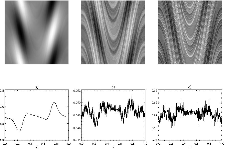
FIG. 1.: Carrying capacity (a), phytoplankton (b) and zooplankton (c) configurations for $a=0.2$ and $T=0$. The upper panels show snapshots of the two-dimensional system, whereas the lower ones display the corresponding concentrations along a horizontal transect taken along $y=0.6$. The smooth character of $C$, and the singular one of $P$ and $Z$, is clearly seen.

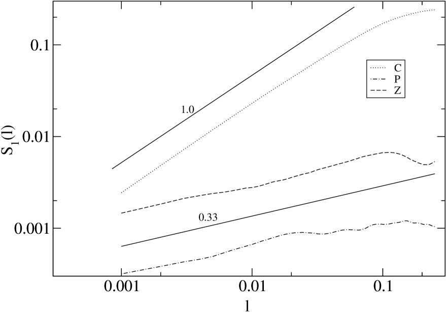
FIG. 2.: First-order structure functions, $S_{1}^{i}(l)$, where $l\equiv\delta x$ is the spatial separation, obtained by averaging over 50 transects in the patterns of Fig. 1. The straight lines are the theoretical predictions for the small scale behavior, and the numbers above them the predicted slopes.

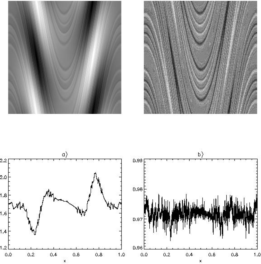
FIG. 3.: Carrying capacity (left) and zooplankton pattern (right) for $a=0.2$ and $T=10$. Both are now rough, but with rather different smoothness properties.

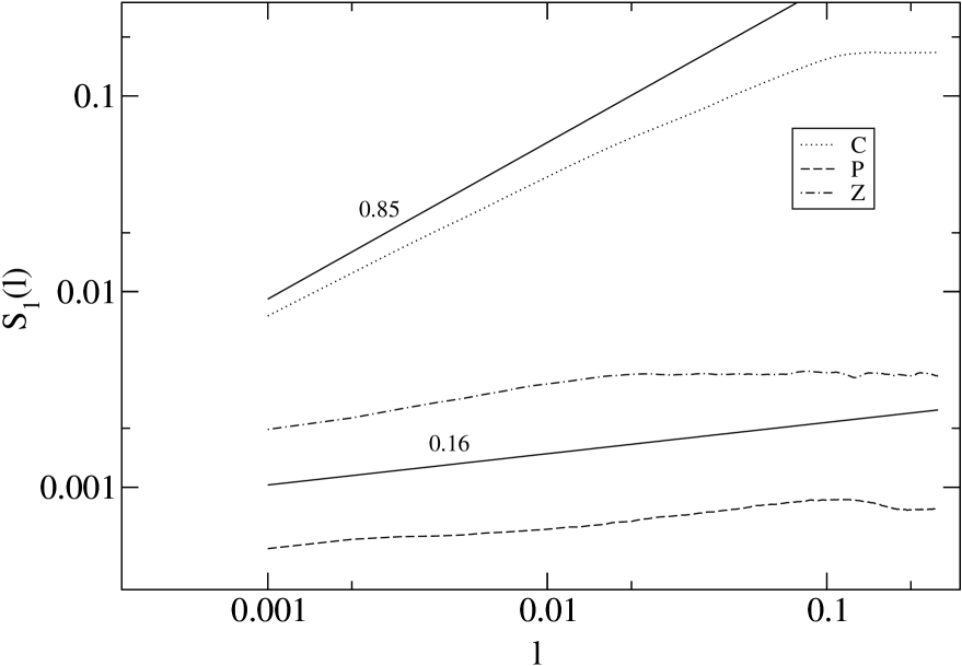
FIG. 4.: Same as Fig. 2, but for the patterns in Fig. 3.

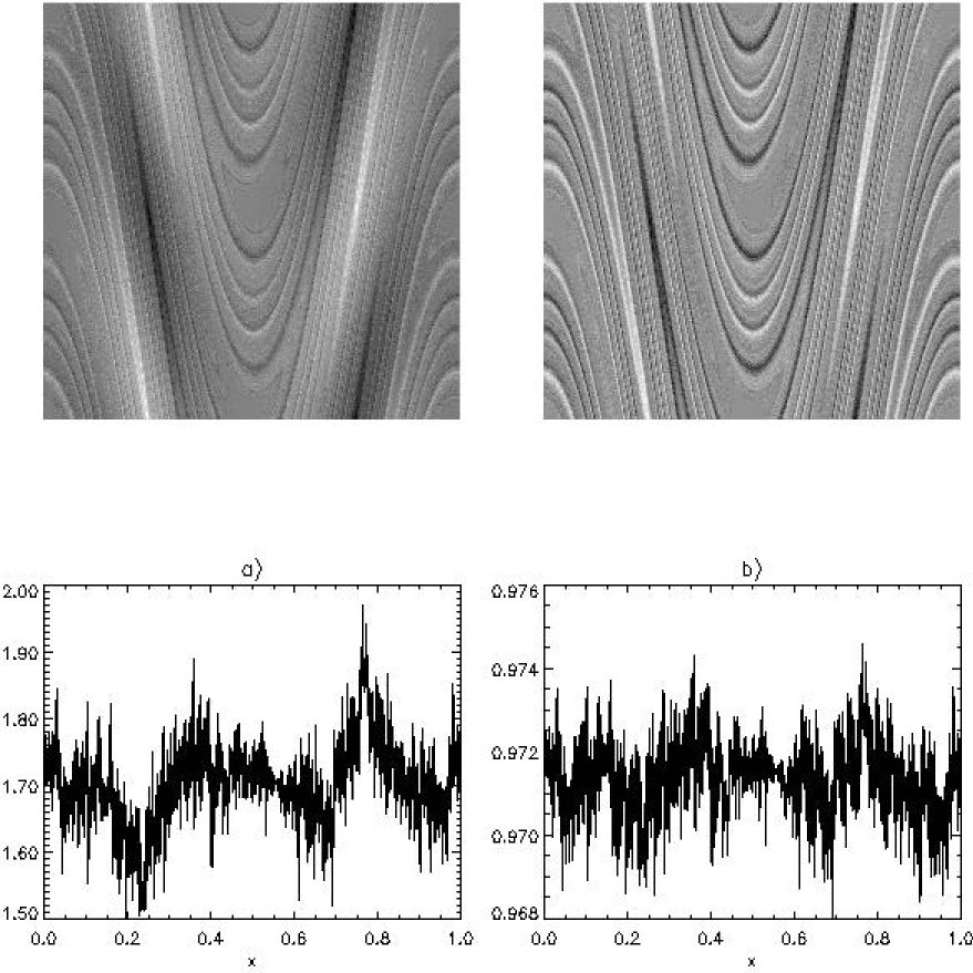
FIG. 5.: Carrying capacity (left) and zooplankton pattern (right) for $a=0.02$ and $T=20$. Both display rough behavior of the same characteristics.

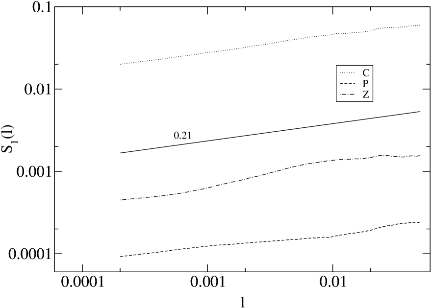
FIG. 6.: Same as Fig. 2, but for the patterns in Fig. 5.

- [1] R.T. Pierrehumbert, Tracer microstructure in the large-eddy dominated regime, Chaos, Solitons and Fractals 4, 1091 (1994).
- [2] J.C. Sommerer, H.-C. Ku and H.E. Gilreath, Experimental evidence for chaotic scattering in a fluid wake, Phys. Rev. Lett. 77, 5055 (1996).
- [3] D. Rothstein, E. Henry, J.P. Gollub, Persistent patterns in transient chaotic fluid mixing, Nature 401, 770 (1999).
- [4] G. A. Voth, G. Haller, and J.P. Gollub, Precision measurements of stretching and compression in fluid mixing, e-print arXiv:nlin.CD/0109006.
- [5] M.G. Balluch and P.H. Haynes, Quantification of lower stratospheric mixing processes using aircraft data, J. Geophys. Res. 102, 23487 (1997).
- [6] Tuck, A.F. and Hovde, S.J. Fractal behavior of ozone, wind speed and temperature in the lower stratosphere. Geophys. Res. Lett. 26, 9 (1999).
- [7] J. H. Steele (ed.). Spatial pattern in plankton communities. Plenum Press, New York (1978); S.A. Levin, T.M. Powell, and J.H. Steele (Eds.), Patch dynamics (Springer-Verlag, Berlin, 1993).
- [8] D.L. Mackas, K.L. Denman, M.R. Abbott, Plankton patchiness: biology in the physical vernacular, Bull. Mar. Sci., 37, 652 (1985).
- [9] G. Károlyi, A. Péntek, I. Scheuring, T. Tél, and Z. Toroczkai, Chaotic flow: The physics of species coexistence, PNAS 97, 13661 (2000).
- [10] Z. Toroczkai, Gy. Károlyi, Á. Péntek, T. Tél and C. Grebogi, Advection of active particles in open chaotic flows, Phys. Rev. Lett. 80, 500 (1998); Gy. Károlyi, Á. Péntek, Z. Toroczkai, T. Tél and C. Grebogi, Chemical or biological activity in open chaotic flows Phys. Rev. E 59, 5468 (1999).
- [11] S. Edouard, B. Legras, F. Lefèvre and R. Eymard, The effect of small-scale inhomogeneties on ozone depletion in the Artic, Nature, 384, 444 (1996).
- [12] A. Mahadevan, D. Archer, Modelling the impact of fronts and mesoscale circulation on the nutrient supply and biogeochemistry of the upper ocean, J. Geophys. Res. 105 C, 1209 (2000).
- [13] K.L. Denman, T. Platt The variance spectrum of phytoplankton in a turbulent ocean, J. Mar. Res. 34, 593 (1976).
- [14] E. R. Abraham, The generation of plankton patchiness by turbulent stirring, Nature 391, 577 (1998).
- [15] Z. Neufeld, Excitable Media in a Chaotic Flow, Phys. Rev. Lett. 87, 108301 (2001).
- [16] B.I. Shraiman and E.D. Siggia Scalar turbulence, Nature 405, 639 (2000).
- [17] G. Falkovich, K. Gawedzki, and M. Vergassola, Particles and fields in fluid turbulence, Rev. Mod. Phys. 73, to appear (2001).
- [18] G.K. Batchelor, Small-scale variation of convected quantities like temperature in turbulent fluid, J. Fluid Mech. 5, 113 (1959).
- [19] H. Aref, Mixing by chaotic advection, J. Fluid Mech. 143, 1 (1984).
- [20] A. Crisanti, M. Falcioni, G. Paladin, and A. Vulpiani, Lagrangian chaos: Transport, mixing, and diffusion in fluids, Rev. Nuovo Cimento 14, 1 (1991).
- [21] J.H.E. Cartwright, M. Feingold, O. Piro, An introduction to chaotic advection, in Mixing: Chaos and Turbulence, Ed. by H. Chaté and E. Villermaux (Kluwer, Dordrecht, 1999).
- [22] P. H. Haynes, Transport, stirring and mixing in the atmosphere in Mixing: Chaos and Turbulence, H. Chaté and E. Villermaux (eds.), Kluwer, Dordretch (1999).
- [23] A. Vulpiani, Lagrangian chaos and small-scale structure of passive scalars, Physica D 38, 372 (1989).
- [24] M. Chertkov, G. Falkovich, I. Kolokolov, and V. Lebedev, Statistics of a passive scalar advected by a large-scale two-dimensional velocity field: Analytic solution, Phys. Rev. E 51, 5609 (1995).
- [25] M.-C. Jullien, P. Castiglione, and P. Tabeling Experimental observation of the Batchelor dispersion of passive tracers, Phys. Rev. Lett. 85, 3636 (2000).
- [26] C. Jung, T. Tél and E. Ziemniak, Application of scattering chaos to particle transport in a hydrodynamical flow, Chaos 3 (4), 555 (1993).
- [27] Á. Péntek, T. Tél and Z. Toroczkai, Chaotic advection in the velocity field of leapfrogging vortex pairs , J. Phys. A 28, 2191 (1995).
- [28] G. Metcalfe and J.M. Ottino, Autocatalytic processes in mixing flows Phys. Rev. Lett. 72, 2875 (1994)
- [29] E. Abraham, A note on the wavenumber spectra of sea-surface temperature and chlorophyll, preprint (1999).
- [30] K. Nam, E. Ott, T.M. Antonsen, Jr., P.N. Guzdar, Lagrangian chaos and the effect of drag on the enstrophy cascade in 2d turbulence, Phys. Rev. Lett. 84, 5134 (2000).
- [31] M. Chertkov, On how the join interaction of two innocent partners (smooth advection and linear damping) produces a strong intermittency, Phys. Fluids 10, 3017 (1998).
- [32] Z. Neufeld, C. López and P.H. Haynes, Smooth-filamental transition of active tracer fields stirred by chaotic advection, Phys. Rev. Lett. 82, 2606 (1999).
- [33] Z. Neufeld, C. López, E. Hernández-García and T. Tél, The multifractal structure of chaotically advected chemical fields, Phys. Rev. E 61, 3857 (2000).
- [34] K. Nam, T.M. Antonsen, Jr., P.N. Guzdar, E. Ott, k-spectrum of finite-lifetime passive scalars in Lagrangian chaotic fluid flows, Phys. Rev. Lett. 83, 3426 (1999).
- [35] S. Corrsin, The reactant concentration spectrum in turbulent mixing with a first-order reaction, J. Fluid Mech. 11, 407 (1961).
- [36] M. Pascual, F.A. Ascioti and H. Caswell, Intermittency in the plankton: a multifractal analysis of zooplankton biomass variability, J. Plankton Res., 17, 1209 (1995).
- [37] L. Seuront, F. Schmitt, Y. Lagadeuc, D. Schertzer, S. Lovejoy and S. Frontier, Multifractal analysis of phytoplankton biomass and temperature in the ocean, Geophys. Res. Lett. 23, 3591 (1996).
- [38] M. Chertkov, Passive advection in nonlinear medium, Phys. Fluids 11, 2257 (1999).
- [39] C. López, Z. Neufeld, E. Hernández-García, P.H. Haynes Chaotic advection of reacting substances: Plankton dynamics on a meandering jet, Phys. Chem. Earth B 26, 313 (2001).
- [40] D.L. Mackas, C.M. Boyd, Spectral analysis of zooplankton spatial heterogeneity, Science 204, 62 (1979).
- [41] J.H. Steele, E.W. Henderson A simple model for plankton patchiness, J. Plank. Res. 14, 1397 (1992).
- [42] C. Marguerit, D. Schertzer, F. Schmmitt, and S. Lovejoy Copepod diffusion within multifractal phytoplankton fields, J. Mar. Sys. 16, 69 (1998).
- [43] J.-P. Eckmann and D. Ruelle, Ergodic theory of chaos and strange attractors, Rev. Mod. Phys. 57, 617 (1985).
- [44] E. Ott, Chaos in dynamical systems, (Cambridge University Press, Cambridge, 1993).
- [45] T. Bohr, M. Jensen, G. Paladin, A. Vulpiani, Dynamical systems approach to turbulence (Cambridge University Press, Cambridge, 1998).
- [46] I. Goldhirsch, P.-L. Sulem, and S.A. Orszag, Stability and Lyapunov stability of dynamical systems: A differential approach and a numerical method, Physica 27 D, 311 (1987).
- [47] C. López, E. Hernández-García, O. Piro, A. Vulpiani, and E. Zambianchi Population dynamics advected by chaotic flows: A discrete-time map approach, CHAOS 11, 397 (2001).
- [48] J.D. Murray, Mathematical Biology, Springer-Verlag, Second Edition, (1993).
- [49] The spatial configurations displayed in the figures have been obtained by integrating until a time , large enough, the chemical subsystem with Lagrangian trajectories that end at spatial points on a regular lattice.
- [50] C. López, E. Hernández-García and Z. Neufeld, The role of diffusion in the chaotic advection of a passive scalar with finite lifetime, preprint (2001).