Discriminating dynamical from additive noise in the Van der Pol oscillator

Abstract

We address the distinction between dynamical and additive noise in time series analysis by making a joint evaluation of both the statistical continuity of the series and the statistical differentiability of the reconstructed measure. Low levels of the latter and high levels of the former indicate the presence of dynamical noise only, while low values of the two are observed as soon as additive noise contaminates the signal. The method is presented through the example of the Van der Pol oscillator, but is expected to be of general validity for continuous-time systems.

, and

1 Introduction

Experimental time series are always blurred with additive noise coming from a variety of sources [1, 2]. Additive noise further complicates time series analysis, leading to ambiguous interpretations of the basic quantities which characterise the dynamics, like correlation dimension and Lyapunov exponents [3, 4]. In particular it may lead unreachable the goal of differentiating deterministic from stochastic dynamics [5, 6, 7, 8, 9, 10, 11].

Here an attempt is made to discriminate additive noise (AN) from the dynamical noise (DN) the system may have. Note that the term additive used here denotes a component of noise that is superimposed to the underlying “clean” signal, due to the measurement process. Common synonyms found in the literature are measurement or observational noise. It should not be confused with the term used in the context of stochastic processes (see, for istance, [12]) where it often indicates a coordinate-independent stochastic forcing as opposite to multiplicative noise, for which the amplitude of the random terms depends on the coordinates themselves. Here we do not focus on this last distinction, and we will denote generically as dynamical every noisy mechanism intrinsic to the system.

Our method is based upon a fundamental, topological, property of deterministic systems, namely, the differentiability of the measure along the reconstructed trajectory [13, 10, 11] or, more specifically, the continuity of its logarithmic derivative. Starting from this basis we show that noise (additive or dynamical) decrease the differentiability of the measure. This would in principle hinder the possibility of differentiating the two types of noise. Then we look at the same property (continuity) of the coordinate. Now, while AN destroys continuity of the coordinate, the latter is scarcely affected by DN. Thus, a low continuity of both the coordinate and (the log derivative of) the reconstructed measure would indicate the presence of AN, while if continuity is high for the coordinate and low for the measure the system contains DN only (see following section). The method, however, doesn’t differentiate sharply a system with the two types of noise from one having solely AN. Notwithstanding, we believe that the present approach is a significant step forward in the understanding of determinism and stochasticity. To illustrate how the method works we consider the simple case of the Van der Pol oscillator [14]. No reasons are forseen that may indicate that the applicability of the method is limited to simple, non chaotic, dynamical systems, such as the one investigated here.

The rest of the paper is organised as follows. In section 2 we make some general considerations on the effects of additive and dynamical noise. In section 3 we briefly discuss the numerical methods followed to solve the dynamical equations with noise and the embedding process. The procedure followed to evaluate the (statistical) continuity is also summarised in that section. The results are discussed in section 4, while section 5 is devoted to the conclusions of our work.

2 General considerations

The method of the reconstructed measure along the trajectory [10, 11] has the capability of revealing the presence of DN in a given time series by looking at the degree of (statistical) continuity of the logarithmic derivative of such a measure. To this end, it is to be considered as complementary to other techniques, essentially based on short-time predictability [5] or on smoothness in phase-space [6, 7, 8]. As far as AN is concerned, in ref. [15] it is argued that methods of the second type can be useful even in real experimental series affected by measurement components. A different line is that followed by Barahona and Poon [16], who are able to cope with rather large amounts of AN, at the “price” of building the analysis upon a given class of Volterra-type nonlinear models adjusted on the time series itself. Here, we do not specify any a priori dynamics and pursue the extension of the method of Ortega and Louis [10, 11] to deal with AN. The choice is motivated by very recent results [17] which allow us to believe that this method is suitable even for high-dimensional chaotic systems, which somehow fool the above-mentioned alternative approaches.

As in refs. [10, 11] we concentrate on continuous-time systems and start by observing that a DN-term modeled by (the increments of) a Wiener process $\delta w_{k}$ (coupled through some constants $G_{jk}$):

$${\rm d}x_{j}=F_{j}(\vec{x}){\rm d}t+\sum_{k}G_{jk}\delta w_{k}$$ (1)

is basically different from white AN, superimposed to the time series $\{s_{n}=s[\vec{x}(n\Delta t)]\}$ after a clean ($G_{jk}=0$) integration:

$$\bar{s}_{n}=s_{n}+\eta_{n}\;.$$ (2)

This is seen in the typical case in which the “measurement function” $s(\vec{x})$ is simply one of the coordinates, say $x_{j}$. In fact, while the white-noise process $\eta_{n}$ of eq. (2) appears to be always discontinuous in time, the $\delta w_{k}$ in eq. (1) lead to a continuous solution, as it can be seen from the increments in a time $\delta t$:

$$x_{j}(t+\delta t)=x_{j}(t)+F_{j}\delta t+\sum_{k}G_{jk}\gamma_{k}(\delta t)^{1/2}+\cdots$$ (3)

The $\gamma_{k}$’s are $\delta$-correlated normal Gaussian random numbers, and in the limit $\delta t\rightarrow 0$ one has $x_{j}(t+\delta t)\rightarrow x_{j}(t)$ [18]. The same applies for a generic (at least differentiable) measurement function, as can be seen from a first-order expansion:

$$s[\vec{x}(t+\delta t)]=s[\vec{x}(t)]+\sum_{j}(\partial_{j}s)[F_{j}\delta t+\sum_{k}G_{jk}\gamma_{k}{(\delta t)}^{1/2}]\;.$$ (4)

Apart from this basic difference, the distinction between AN and DN in the real output of a numerical integration (or of an experimental device) is still a complicated task because the continuity must be judged on the basis of finite increments $\Delta t$ over which the series acquires a finite increment $\Delta s$. From this point of view, the continuity statistics (CS) of Pecora et al. [11, 13] sheds some light as it evaluates the degree of continuity at different resolution scales.

Before closing the section we draw some comments on another type of problem which is sometimes put forth [19, 2], namely, that the distinction between AN and DN is not well-posed since (at least in some cases) they can be mapped onto each other. Consider a discrete-time dynamics with some noisy feedback $\vec{\gamma}$:

$$\vec{x}_{n+1}=\vec{f}\left(\vec{x}_{n}\right)+\vec{\gamma}_{n+1}\;,\;\;n=0,1,\dots$$ (5)

In absence of DN the clean time series from the $j$-th coordinate would be:

$$s_{0}=x_{0j}\,,\;s_{1}=f_{j}\left(\vec{x}_{0}\right),\;s_{2}=f_{j}\left(\vec{f}\left(\vec{x}_{0}\right)\right),\;s_{3}=f_{j}\left(\vec{f}\left(\vec{f}\left(\vec{x}_{0}\right)\right)\right),\;\dots$$ (6)

whereas DN turns it to:

$$\bar{s}_{0}=x_{0j}\,,\;\bar{s}_{1}=f_{j}\left(\vec{x}_{0}\right)+\gamma_{1j},\;\bar{s}_{2}=f_{j}\left(\vec{f}\left(\vec{x}_{0}\right)+\vec{\gamma}_{1}\right)+\gamma_{2j},$$

$$\bar{s}_{3}=f_{j}\left(\vec{f}\left(\vec{f}\left(\vec{x}_{0}\right)+\vec{\gamma}_{1}\right)+\vec{\gamma}_{2}\right)+\gamma_{3j}\;\dots$$ (7)

Now, by the light of eq. (2), one could equally say that the time series (7) stems from a deterministic dynamics $\vec{x}_{n+1}=\vec{f}\left(\vec{x}_{n}\right)$ plus the following (equivalent) AN:

$$\eta_{1}=\gamma_{1j},\;\eta_{2}=\gamma_{2j}+f_{j}\left(\vec{f}\left(\vec{x}_{0}\right)+\vec{\gamma}_{1}\right)-f_{j}\left(\vec{f}\left(\vec{x}_{0}\right)\right),\;$$

$$\eta_{3}=\gamma_{3j}+f_{j}\left(\vec{f}\left(\vec{f}\left(\vec{x}_{0}\right)+\vec{\gamma}_{1}\right)+\vec{\gamma}_{2}\right)-f_{j}\left(\vec{f}\left(\vec{f}\left(\vec{x}_{0}\right)\right)\right)$$ (8)

Similar arguments apply to more general measurement functions and also to continuous-time systems, at least at the leading order of eq. (4). Thus, in principle it is conceivable that a special type of AN can mimic a given DN present in the dynamics. However, from a practical point of view, a measurement noise like the one in eq. (8) is not too realistic, as it is “customised” on the dynamics itself (through $\vec{f}$) and on the initial conditions (in the case of continuous-time systems it would also scale with the integration time). In addition, what is more important is that the process in eq. (8) is autocorrelated, as can be seen by inverting the relationship between the $\vec{\gamma}$’s and the $\eta$’s step by step. Again, the autocorrelation pattern is determined by dynamical features of the system in a complicated way and in general it does not correspond to a typical measurement component. Thus, being conscious of the mathematical subtleties which may arise in rigorous framework, in what follows we restrict to white noise processes as a first possible modelisation of real situations.

3 Model and Numerical Procedures

3.1 The Van der Pol oscillator

The different effects of AN and DN have been tested on the Van der Pol system, whose “clean” equations are:

$$\dot{y}=-\mu(x^{2}-1)y-x$$

$$\dot{x}=y$$ (9)

The white noise, added either to the left-hand sides of eqs. (9) or to the clean coordinate $x$, is generated using a Gaussian distribution with zero mean. Different values of the variance, $\sigma^{2}$, have been considered in order to tune the strength of the noisy terms. We point out that from the discussion of the previous section, and from the following results, there are no apparent obstacles to extend these ideas to high-dimensional/chaotic systems. The reason why we choose such a simple system is that, due to its one-dimensional attractor, we can clarify the points without worrying about the problems of “wandering” [11] which may arise when the embedding dimension is pushed at higher and higher values.

3.2 Numerics

The initial conditions for the system (9) have been set to $(x_{0}=1,y_{0}=0)$ and $\mu=1$. These choices lead to a “clean” amplitude of oscillation of about 2, with period 6.6. Dealing with stochastic differential equations, we used an Euler integration scheme to produce time-series of 16384 points from the $x$ coordinate. To achieve a good compromise in terms of numerical accuracy we choosed an integration time step $\Delta t=0.01$. The transient time was observed to be sufficient for the oscillator to relax on the 1D attractor. Numerically we explored embedding dimension $m$ up to 10, using a delay time of 166 which corresponds to the first zero of the autocorrelation function (in units of $\Delta t$). As in [11], we adopt an Epanechnikov kernel measure estimator with a radius of 0.05 (after that the reconstructed attractor has been rescaled to lie within the hypercube $[0,1]\times\cdots\times[0,1]$).

3.3 Continuity statistics

In order to test the mathematical properties embodied in a possible mapping between two given time series, that is, continuity, differentiability, inverse differentiability and injectivity, Pecora et al. [13] have developed a set of statistics aimed to test quantitatively these features. Their algorithms are of general use and can in particular be applied to test topological properties in any pair of sets of points. Basically, the method is intended to evaluate, in terms of probability or confidence levels, whether two data sets are related by a mapping having the continuity property: A function $f$ is said to be continuous at a point $\vec{x}_{0}$ if $\forall\varepsilon>0,\exists\delta>0$ such that $\parallel\vec{x}-\vec{x}_{0}\parallel<\delta\Rightarrow\parallel f(\vec{x}))-f(\vec{x}_{0})\parallel<\varepsilon$. The results are tested against the null–hypothesis, specifically, the case in which no functional relation exists. This is done by means of the statistics proposed by Pecora et al. [13]

$$\Theta_{C^{0}}(\varepsilon)=\frac{1}{n_{p}}\sum_{j=1}^{n_{p}}\Theta_{C^{0}}(\varepsilon,j)$$ (10)

and

$$\Theta_{C^{0}}(\varepsilon,j)=1-\frac{p_{j}}{P_{\rm max}}$$ (11)

where $p_{j}$ is the probability that all of $n_{\delta}$ points in the $\delta$-set, around a certain point $\vec{x}_{j}$, fall in the $\varepsilon$-set around $f(\vec{x}_{j})$. The likelihood that this will happen must be relative to the probability, $P_{\rm max}$, of the most likely event under the null hypothesis. In the Appendix we present some details on the calculation of the ratio in eq. (11), useful for a numerical implementation. The sum in eq. (10) represent an average over $n_{p}$ points chosen at random in the whole time series. Now, when $\Theta_{C^{0}}(\varepsilon)\approx 1$ we can confidently reject the null hypothesis, and assume that there exists a continuous function. As in the work of Pecora et al. [13] the $\varepsilon$ scale is relative to the standard deviation of the time series, and thus $\varepsilon\in[0,1]$. Plots of $\Theta_{C^{0}}(\varepsilon)$ versus $\varepsilon$ can be used to quantify the degree of statistical continuity of a given function. In order to characterise the continuity statistics by means of a single parameter we have also calculated,

$$\theta=\int_{0}^{1}\Theta_{C^{0}}(\varepsilon){\rm d}\varepsilon$$ (12)

The limiting values of $\theta$, namely, 0 and 1, correspond to a strongly discontinuous and a fully continuous function, respectively. In the results reported here the function $f$ mentioned above can be either the logarithmic derivative of the measure or the coordinate itself. When useful, we will denote the corresponding continuity statistics by CSLDM and CSC. The resolution scale $\varepsilon$ varied in the range $[0.0001,1]$ and $n_{p}$ was always fixed to be a 20% of the total length of the series.

4 Results

The CSC for the amplitude $x$ of the Van der Pol oscillator (eqs. (9)) is shown in fig. 1 for different levels and kinds of noise. On the one hand it is readily seen that the CSC for the time series affected by DN is essentially independent of the noise amplitude. This appears to be consistent with the continuity analysis sketched in section 2. On the other hand, the CSC for series affected by AN decreases steadily, and almost linearly, with the noise level $\sigma_{\rm AN}$. We have considered also the more subtle case in which both AN and DN are present. In particular, we have fixed a moderate level of DN, like $\sigma_{\rm DN}=0.1$, and then contaminated the resulting $x$-time series with various levels of AN. The corresponding points in fig. 1 are almost indistinguishable from those without DN, indicating that what rules the CSC is the presence of AN. To give an idea of how the CS is disributed over the different resolution scales we have plotted, in fig. 2, the $\Theta_{C^{0}}$ statistics of the coordinate for some representative cases. Roughly we could say that the effect of the various noise sources is to shift, along the $\varepsilon$ axe, the same sigmoidal shape. What is different, between AN and DN, is that the shift induced by the former is considerably more pronounced, actually one order of magnitude in $\varepsilon$ when passing from $\sigma_{\rm AN}=0.03$ to $\sigma_{\rm AN}=0.3$.

Let us now come to the analysis of the CSLDM values. In refs. [11, 17] it was argued that this quantity is an indicator which is sensible to the presence of DN. The results of fig. 3 show that it is also strongly affected by AN. Both the DN- and the AN-data decrease almost monotonically with the noise level, with the exception of a small jump at $\sigma=0.09$. The origin of the latter is not completely clear, though it may be partially due to the statistical fluctuations induced by the sampling over the $n_{p}$ points (eq. (10)). As in fig. 1 we present some cases in which the combined action of AN and DN takes place, just to show a limitation of the present approach. The pure AN and the AN+DN data are not so close as in fig. 1 but there is not a definite trend to discriminate between a non-stochastic ($\sigma_{\rm DN}=0$) and a stochastic underlying dynamics, when the original time series is contaminated by AN. As a general property we should note that the AN-free values are always greater than the ones in which AN is present. For the sake of completeness a $\Theta$-vs-$\varepsilon$ plot for the measure is given in fig. 4. With respect to fig. 2 the sigmoidal shape is flattened (rather than shifted), and the AN curves are somehow less regular than the DN ones. Nonetheless, the lowering effect of noise is clearly appreciable. Note also that in this case the effect of varying the AN level of one order of magnitude is far less evident than in the CSC. In fact this is consistent with fig. 3 where it is seen that the CSLDM jumps down and levels off to $\simeq 0.3$ as soon as a small amount of AN is introduced.

5 Conclusions

In this paper we have presented the extension of the method of refs. [10, 11] to the analysis of time series affected by AN. The basic task which one has to perform is to compare the behaviour of the statistical continuity of the coordinate and of the statistical differentiabilty of the natural measure, at different levels of noise. While the first is sensibly different from the “clean” one only when AN is present, the second is affected by both dynamical and additive noise. Hence, it is possible to discriminate between the two cases. Altough we believe that the present method can be readily applied also to high-dimensional and/or chaotic systems, the results discussed here refer to the simple Van der Pol oscillator. A further key step in the analysis of experimental time series, namely the criterion to adopt when both types of noise are present, has been only touched here and is currently investigated by means of real physiological data.

6 Acknowledgements

This work was supported by grants of the spanish CICYT (grant no. PB96–0085), the European TMR Network-Fractals c.n. FMRXCT980183, the Universidad Nacional de Quilmes (Argentina) and the Universidad de Alicante (Spain). G. Ortega is a member of CONICET Argentina.

7 Appendix

As pointed out in [13] the appropriate probability distribution for the continuity test is the binomial one:

$$P(k;p,n_{\delta})=\frac{n_{\delta}!}{k!(n_{\delta}-k)!}p^{k}(1-p)^{n_{\delta}-k}\;,\;\;k=0,1,\dots,n_{\delta}\;,$$ (13)

with $p=n_{\varepsilon}/N$, $n_{\varepsilon}$ being the number of points in $\varepsilon$-set (see text). In addition, due to the null hypotesis under consideration, the probility $p_{j}$ appearing in eq. (11) is just $p_{j}=p^{n_{\delta}}$. Except for the trivial case $p=1$, for which one has $P(k)=\delta_{k,n_{\delta}}$, the maximum of the distribution (13) is located at $k_{\rm max}=[p(n_{\delta}+1)]$ ($[\;\cdot\;]$ denoting the integer part - see, for istance, [20]). Now, let us observe that in the present case we must calculate only the ratio:

$$\frac{p^{n_{\delta}}}{P_{\rm max}}=\frac{k_{\rm max}!(n_{\delta}-k_{\rm max})!}{n_{\delta}!}\rho^{n_{\delta}-m_{\rm max}}\;,$$ (14)

where $\rho=p/(1-p)$. ¿From a numerical point of view it is advantageous to exploit the following trick in the left-hand side of eq. (14). Take $M=\max{(k_{\rm max},n_{\delta}-k_{\rm max})}$, so that $M!$ can be simplified in the numerator and in the denominator of the fraction leaving:

$$\frac{k_{\rm max}!(n_{\delta}-k_{\rm max})!}{n_{\delta}!}=\frac{(n_{\delta}-M)!}{n_{\delta}(n_{\delta}-1)\dots(M+1)}=\prod_{\ell=1}^{n_{\delta}-M}\frac{\ell}{\ell+M}\;.$$ (15)

Dealing with the product in eq. (15) has the advantage of avoiding ratios of very large numbers. However, the powers of $\rho$ appearing in eq. (14) can still introduce rather small numbers, which have to be treated through their logarithms.

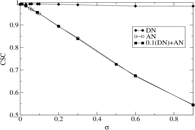
Figure 1: CSC versus noise standard deviation, $\sigma$, for the $x$ coordinate of the Van der Pol oscillator. Results are shown for pure AN (no DN, open circles), pure DN (no AN, full diamonds) and for a system having a fixed level $\sigma_{\rm DN}=0.1$ plus AN with variable standard deviation (full squares, almost overlapped with the open circles).

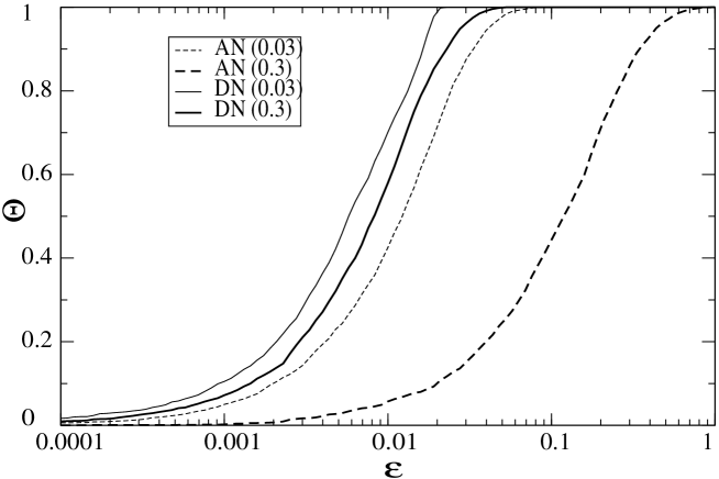
Figure 2: CSC resolved at different $\varepsilon$ scales. The legend indicates the type and the levels (standard deviation) of noise.

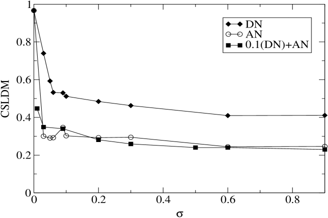
Figure 3: CSLDM versus noise standard deviation, $\sigma$, corresponding to a four-dimensional embedding (the other paramters being reported in the main text). Results are shown for pure AN (no DN, open circles), pure DN (no AN, full diamonds) and for a system having a fixed level $\sigma_{\rm DN}=0.1$ plus an AN with variable standard deviation (full squares).

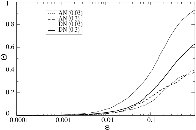
Figure 4: CSLDM resolved at different $\varepsilon$ scales, for the same levels and types of noise of Fig. 2. In all cases, the measure is estimated from a four-dimensional embedding with the parameters indicated in the text.

References

- [1] A.S. Weigend and N.A. Gershenfeld (editors), Time series Prediction, Santa Fe Institute Studies in the Sciences of Complexity series, vol. XV (Addison Wesley, Reading, 1994).
- [2] H. Kantz and T. Schreiber, Nonlinear Time Series Analysis (Cambridge University Press, Cambridge, 1997).
- [3] H. Kantz, pp. 475-490 in [1].
- [4] T. D. Sauer and J. A. Yorke, Phys. Rev. Lett. 83, 1331 (1999).
- [5] G. Sugihara and R. May, Nature (London) 344, 734 (1990).
- [6] D.T. Kaplan and L. Glass, Phys. Rev. Lett. 68, 427 (1992); Physica D 64, 431 (1993).
- [7] R. Wayland, D. Bromley, D. Pickett and A. Passamante, Phys. Rev. Lett. 70, 580 (1993).
- [8] L.W. Salvino and R. Cawley, Phys. Rev. Lett. 73, 1091 (1994).
- [9] J. Bhattacharya and P. P. Kanjil, Physica D 132, 100 (1999).
- [10] G. Ortega and E. Louis, Phys. Rev. Lett. 81, 4345 (1998).
- [11] G. Ortega and E. Louis, Phys. Rev. E. 62, 3419 (2000).
- [12] M. San Miguel and R. Toral, in Instabilities and Nonequilibrium Structures, Vol. VI, E. Tirapegui and W. Zeller eds. (Kluwer Academic Pub., 1997).
- [13] L. Pecora, T. Carroll and J. Heagy, Phys. Rev. E. 52, 3420 (1995).
- [14] T. Sauer y J. Yorke, Ergodic Th. Dyn. Syst. 17, 941 (1997).
- [15] T. Miyano, Int. J. Bif. Chaos, 6, 2031 (1996)
- [16] M. Barahona and C.-S. Poon, Nature 381, 215 (1996).
- [17] G. Ortega, C. Degli Esposti Boschi and E. Louis, “Detecting determinism in high-dimensional chaotic systems”, submitted to Phys. Rev. E.
- [18] Note that in eq. (3) we have assumed that the are independent of . However, the generalisation to the -dependent case does not modify our picture since the essential point for the continuity property is the existence of a term. This turn out to be the case when the increments are calculated through the Milshtein scheme [12].
- [19] G. G. Szpiro, Physica D 65, 289 (1993).
- [20] A. M. Mood, F. A. Graybill and D. C. Boes, Introduction to the theory of statistics (McGraw Hill, Inc., 1974).
- [21] H. Abarbanel, R. Brown, J. Sidorowich and L. Tsimring, Rev. Mod. Phys. 65, 1331 (1993).
- [22] M. Cencini, M. Falcioni, E. Olbrich, H. Kantz and A. Vulpiani, Phys. Rev. E 62, 427 (2000).
- [23] J. Jeong, M.S. Kim and S.Y. Kim, Phys. Rev. E 60, 831 (1999).
- [24] M. Ding et al. Physica D 69, 404 (1993).
- [25] A. Galka, T. Maab and G. Pfister, Physica D, 121, 237 (1998).
- [26] M. Casdagli, S. Eubank, D. Farmer and J. Gibson, Physica D 51, 52 (1991).
- [27] R. Hegger, M. J. Bünner and H. Kantz, Phys. Rev. Lett. 81(3), 558 (1998).
- [28] E. Olbrich and H. Kantz, Phys. Lett. A 232(1-2), 63 (1997).
- [29] J. Theiler, S. Eubank, A. Longtin, B. Galdrikian and J. D. Farmer, Physica D 58, 77 (1992).
- [30] A. Osborne and A. Provenzale, Physica D 35, 357 (1989).
- [31] T. Schreiber, Phys. Rev. Lett 80, 2105 (1998).