Generic features of modulational instability in nonlocal Kerr media.

Abstract

The modulational instability (MI) of plane waves in nonlocal Kerr media is studied for a general, localized, response function. It is shown that there always exists a finite number of well-separated MI gain bands, with each of them characterised by a unique maximal growth rate. This is a general property and is demonstrated here for the Gaussian, exponential, and rectangular response functions. In case of a focusing nonlinearity it is shown that although the nonlocality tends to suppress MI, it can never remove it completely, irrespectively of the particular shape of the response function. For a defocusing nonlinearity the stability properties depend sensitively on the profile of the response function. It is shown that plane waves are always stable for response functions with a positive-definite spectrum, such as Gaussians and exponentials. On the other hand, response functions whose spectra change sign (e.g., rectangular) will lead to MI in the high wavenumber regime, provided the typical length scale of the response function exceeds a certain threshold. Finally, we address the case of generalized multi-component response functions consisting of a weighted sum of N response functions with known properties .

OCIS codes: 190.5530, 190.4420, 190.5940.

I Introduction

The phenomena of modulational instability (MI) of plane waves has been identified and studied in various physical systems, such as fluids [1], plasma [2], nonlinear optics [3, 4], discrete nonlinear systems, such as molecular chains [5] and Fermi-resonant interfaces and waveguide arrays [6], dispersive nonlinear directional couplers with the change of refractive index following a exponential relaxation law [7] etc. It has been shown that MI is strongly affected by various mechanisms present in nonlinear systems, such as higher order dispersive terms in the case of optical pulses [8], saturation of the nonlinearity [9], and coherence properties of optical beams [10].

In this work we study the MI of plane waves propagating in a nonlinear Kerr type medium with a nonlinearity (the refractive index change, in nonlinear optics) that is a nonlocal function of the incident field. We consider a phenomenological model

$$i\partial_{z}\psi+\frac{1}{2}\partial_{x}^{2}\psi+s\psi\int_{-\infty}^{\infty}R(x^{\prime}-x)|\psi(x^{\prime})|^{2}dx^{\prime}=0,$$ (1)

for the wave modulation $\psi$ where $x$ is the transverse spatial coordinate and $s=1$ $(s=-1)$ corresponds to a focusing (defocusing) nonlinearity. The evolution coordinate $z$ can be time, as for Bose-Einstein Condensates (BEC’s), or the propagation coordinate, as for optical beams. We consider only symmetric spatial response functions that are positive definite and (without loss of generality) obey the normalization condition

$$\int_{-\infty}^{\infty}R(x)dx=1.$$ (2)

Thus we exclude asymmetric effects, such as those generated by asymmetric temporal response functions (with $x$ being time), as in the case of the Raman effect on optical pulses [11].

In nonlinear optics (1) represents a general phenomenological model for media in which the nonlinear refractive index change (or polarization) induced by an optical beam is determined by some kind of a transport process. It may include, e.g., heat conduction in materials with a thermal nonlinearity [12, 13, 14] or diffusion of molecules or atoms accompanying nonlinear light propagation in atomic vapours [15]. Nonlocality also accompanies the propagation of waves in plasma [16, 17, 18, 19, 20], and a nonlocal response in the form (1) appears naturally as a result of many body interaction processes in the description of Bose-Einstein condensates [21].

The width of the response function $R(x)$ relative to the width of the intensity profile $|\psi|^{2}(x,z)$ determines the degree of nonlocality. In the limit of a singular response we get the well-known nonlinear Schrödinger (NLS) equation, which appears in all areas of physics. Here the focusing case ($s$=1) produces MI of the finite bandwidth type, while the defocusing case ($s$=$-1$) predicts modulational stability [3]. When the width of the response function is finite but small compared to the intensity, the model (1) is approximated by the modified NLS equation [22, 23, 24, 25, 26]

$$i\partial_{z}\psi+\frac{1}{2}\partial_{x}^{2}\psi+s[|\psi|^{2}+\gamma\partial_{x}^{2}|\psi|^{2}]\psi=0.$$ (3)

Here $\gamma\ll 1$ is defined as the second virial of $R(x)$ as

$$\gamma\equiv\frac{1}{2}\int_{-\infty}^{\infty}x^{2}R\left(x\right)dx$$ (4)

and it scales as $\gamma\sim\sigma^{2},$ where $\sigma$ is the characteristic length of the response function. In contrast to the local NLS limit ($\gamma$=0), the MI now depends not only on the sign of $s$, but also on the intensity of the plane waves [17]. Finally, in the case of strong nonlocality it has been shown that (1) simplifies to a linear model, and hence there is no MI in this limit [27].

MI has thus been studied in different limits. The general case (1) has recently been investigated with respect to MI and compared with the weakly nonlocal limit [22]. Here we present an analytical study of the full nonlocal case with arbitrary profile $R(x)$ whose spectrum obeys a sufficient degree of smoothness, with particular emphasis on generic features of the MI. The present paper complements and extends the results obtained in [22].

II MI in the nonlocal NLS equation

The model (1) permits plane wave solutions of the form

$$\psi(x,z)=\sqrt{\rho_{0}}\exp(ik_{0}x-i\omega_{0}z),\quad\rho_{0}>0,$$ (5)

where $\rho_{0}$, $k_{0}$, and $\omega_{0}$ are linked through the nonlinear dispersion relation

$$\omega_{0}=\frac{1}{2}k_{0}^{2}-s\rho_{0},$$ (6)

Following [22], we perturb the plane wave solutions (5) - (6) as follows: Assume that

$$\psi\left(x,z\right) = \left[\sqrt{\rho_{0}}+u\left(\xi,\tau\right)+iv\left(\xi,\tau\right)\right]\exp(i\theta_{0})$$ (7)

$$\xi = x-k_{0}z,\text{ }\tau=z,$$ (8)

$$\theta_{0} = k_{0}x-\omega_{0}z,$$ (9)

where $u$ and $v$ denote the real- and imaginary part of the perturbation. Inserting this expression into the nonlocal NLS equation (1) and linearizing around the solution (5) - (6) yields the equations

$$\begin{array}[]{c}\partial_{\tau}u+\frac{1}{2}\partial_{\xi}^{2}v=0,\\ \\ \partial_{\tau}v-\frac{1}{2}\partial_{\xi}^{2}u-2s\rho_{0}\int_{-\infty}^{\infty}R(\xi^{\prime}-\xi)u(\xi^{\prime},\tau)d\xi^{\prime}=0,\end{array}$$ (10)

for the perturbations $u$ and $v.$  By introducing the Fourier transforms

$$\widehat{u}(k,\tau) = \int_{-\infty}^{\infty}u(\xi,\tau)\exp[ik\xi]d\xi,$$ (11)

$$\widehat{v}(k,\tau) = \int_{-\infty}^{\infty}v(\xi,\tau)\exp[ik\xi]d\xi,$$ (12)

$$\widehat{R}(k) = \int_{-\infty}^{\infty}R(\xi)\exp[ik\xi]d\xi,$$ (13)

and exploiting the convolution theorem for Fourier transforms, the linearized system is converted to a set of ordinary differential equations in $k$-space

$$\begin{array}[]{c}\partial_{\tau}\widehat{u}-\frac{1}{2}k^{2}\widehat{v}=0,\\ \\ \partial_{\tau}\widehat{v}+\frac{1}{2}k^{2}\widehat{u}-2s\rho_{0}\widehat{R}\,\widehat{u}=0,\end{array}$$ (14)

which can be written in the compact matrix form

$$\partial_{\tau}\underline{X}=\underline{\underline{A}}\;\underline{X},$$ (15)

where the vector $\underline{X}$ and matrix $\underline{\underline{A}}$ are defined as

$$\underline{X}=\left[\begin{array}[]{c}\widehat{u}\\ \widehat{v}\end{array}\right],\;\underline{\underline{A}}=\left[\begin{array}[]{cc}0&\frac{1}{2}k^{2}\\ -\frac{1}{2}k^{2}+2s\rho_{0}\widehat{R}(k)&0\end{array}\right].$$ (16)

The eigenvalues $\lambda$ of the matrix $\underline{\underline{A}}$ are given by

$$\lambda^{2}=k^{2}\rho_{0}\left[s\widehat{R}(k)-\frac{1}{4\rho_{0}}k^{2}\right].$$ (17)

The general dispersion relation (17) constitutes the basis of our study of MI.

Let us summarize the properties of the spectrum $\widehat{R}(k)$:

1. Since $R(x)$ is realvalued and symmetric, then so is $\widehat{R}(k)$, i.e. $\widehat{R}(k)=\widehat{R}(-k)=\widehat{R}^{\ast}(k)$.

2. The normalization (2) implies $\widehat{R}(0)$=1.

3. The symmetry condition for the Fourier transforms imposes $\widehat{R}^{\prime}(0)$=0, i.e. the spectrum has a critical point at $k$=0. Here and in the following prime denotes differentiation with respect to the argument.

4. The normalization (2) for $R(x)$ means by assumption that $R(x)$ is absolute integrable, and hence by Riemann - Lebesque lemma we have $\lim_{k\rightarrow\infty}\widehat{R}(k)=0$ [28].

5. The functions $R(x)$, $xR(x)$ and $x^{2}R(x)$ are assumed to be absolute integrable, and thus by [28] $\widehat{R}(k)$, $\widehat{R}^{\prime}(k)$, and $\widehat{R}^{\prime\prime}(k)$ are continuous for all $k$.

6. The response functions are characterized by typical widths and scaling lengths $\sigma$ and they assume the generic form $R(x)=\sigma^{-1}\Phi(x/\sigma)$, where $\Phi$ is a non-dimensional scaling function.

The spectrum $\widehat{R}\left(k\right)$ can be expressed in terms of the Fourier - transform $\widehat{\Phi}$ of the scaling function $\Phi$ as

$$\widehat{R}\left(k\right)=\widehat{\Phi}\left(\sigma k\right)\equiv\int_{-\infty}^{\infty}\Phi\left(\zeta\right)\exp\left[i\sigma k\zeta\right]d\zeta.$$ (18)

Notice that the list of general properties 1-6 of the spectrum $\widehat{R}$ carries over to $\widehat{\Phi}$.

The dispersion relation (17) is now conveniently rewritten as

$$\lambda^{2}/\lambda_{0}^{2}=k^{2}\phi\left(k;s,\sigma\right),\text{ }$$ (19)

by means of (18), the definition

$$\lambda_{0}\equiv 2\rho_{0}$$ (20)

the redefinitions

$$2\sqrt{\rho_{0}}\sigma\rightarrow\text{ }\sigma,\text{ }\frac{1}{2\sqrt{\rho_{0}}}k\rightarrow k$$ (21)

and

$$\phi\left(k;s,\sigma\right)\equiv s\widehat{\Phi}\left(\sigma k\right)-k^{2}$$ (22)

The parameter $\sigma$ which measures the width of the response function, plays the role as a control parameter. Observe that $\widehat{\Phi}$ is a continuous differentiable function of $k.$ The crucial point in the stability analysis is the properties of the function $\phi.$ More precisely, by appealing to the list of properties 1-6 we can characterize the set $\Omega$ of $k$ fulfilling the inequality $\phi\left(k;s,\sigma\right)\geq 0$ for a given value of $\sigma$ as follows:

• If $\phi\left(k\right)<0$ for all $k\geq 0,$ then $\Omega$ is empty. In this case we have modulational stability.

• If the transversality condition $\phi^{\prime}\neq 0$is satisfied at the zeros of $\phi,$ the number of zeros is finite. In addition, these points are distinct and isolated. In this case $\Omega$ is given as a finite union of well-separated, closed, bounded subintervals of the positive $k$ - axis. In this case we have MI of the finite bandwidth type.

• The breakdown of the transversality condition for certain values of $\sigma$, i.e.,

  $$\phi\left(k\right)=\phi^{\prime}\left(k\right)=0\text{ for }k=k_{c},\sigma=\sigma_{c}$$ (23)

  describes bifurcation phenomena like excitation, vanishing, coalescence, and separation of MI bands. A careful analysis of the behavior of $\phi$ in the neighborhood of the bifurcation point will reveal the type of phenomena which takes place. The number of zeros of $\phi$ will change as $\sigma$ passes the critical value $\sigma_{c}$. The case $\phi^{\prime\prime}\left(k_{c}\right)>0$ for $\sigma=\sigma_{c}$, can be interpreted as a condition for two MI bands to merge together or that one single MI band separates into two gain bands, while $\phi^{\prime\prime}\left(k_{c}\right)<0$ for $\sigma=\sigma_{c}$ represents excitation or vanishing of an MI band. The critical value $\sigma_{c}$ and the type of bifurcation can be determined as follows:  Solve the equation

  $$z\widehat{\Phi}^{\prime}\left(z\right)=2\widehat{\Phi}\left(z\right),\text{ }z>0$$ (24)

  Then the widths $\sigma_{c}$ can be expressed as

  $$\sigma_{c}=\frac{z}{\sqrt{s\widehat{\Phi}\left(z\right)}}$$ (25)

  provided $s\widehat{\Phi}\left(z\right)>0.$ The second derivative of $\phi$ evaluated at the bifurcation point can also be expressed in terms of $z:$

  $$\phi^{\prime\prime}=\frac{z^{2}\widehat{\Phi}^{\prime\prime}\left(z\right)}{\widehat{\Phi}\left(z\right)}-2$$ (26)

From now on we will assume that the transversality condition is satisfied at the zeros of $\phi,$ except for a set of isolated bifurcation points. This means that the behavior of the graph of   spectrum $\widehat{\Phi}\left(\sigma k\right)$ relative to the parabola $k^{2}$ determines the stability properties. We will discuss this aspect in more detail in the coming subsections. Let us first assume that $\phi\left(k;s,\sigma\right)\geq 0$ for some positive $k$. For such values of $k$ the normalized growth rate $\Gamma$ reads

$$\Gamma=\left|{\cal Re}\left(\lambda\right)\right|/\lambda_{0}=\left|k\right|\sqrt{\phi\left(k;s,\sigma\right)}$$ (27)

In the present paper we will consider situations where the MI of the nonlocal NLS equation is of finite bandwidth type and that each gain band has a unique maximum growth rate, in the same as we have for the MI of the focusing NLS model and the weakly nonlocal limit, and it emerges as a generic property for a large class of response functions like the Gaussian, the exponentially decay function and the square pulse function. It is straightforward to derive the conditions which must be fulfilled: We find

$$\Gamma^{\prime}=\frac{1}{2}\phi^{-1/2}\left[2\phi+k\phi^{\prime}\right]$$ (28)

and hence the maximum point $k=$ $k_{\max}$ obeys

$$\left[2\phi+k\phi^{\prime}\right]_{k=k_{\max}}=0$$ (29)

The second derivative of $\Gamma$ at $k=$ $k_{\max}$ is given as

$$\Gamma^{\prime\prime}=\frac{1}{2}\phi^{-1/2}\left[3\phi^{\prime}+k\phi^{\prime\prime}\right]_{k=k_{\max}}$$ (30)

and in order to have a local maximum at $k=$ $k_{\max}$ the function $\phi$ must obey the inequality

$$\left[3\phi^{\prime}+k\phi^{\prime\prime}\right]_{k=k_{\max}}<0$$ (31)

The condition (31) is referred to as the generic condition for the existence of a maximum growth rate. One can prove that if all the critical points of $\Gamma$ obey (31), these points coincide, and hence we have an MI pattern which resembles the MI of the local, focusing NLS.

II.1 The focusing case (s=1)

In this case the function $\phi$ defined by (22) appearing in (19) and (27) is given as

$$\phi\equiv\widehat{\Phi}\left(\sigma k\right)-k^{2}$$ (32)

From the list of general properties we find that $\phi\left(0\right)=1$ and we can prove that the number of zeros of $\phi$, denoted by $N$, is odd, i.e. $N=2m-1$ $\left(m=1,2,..\right)$ and that there are $m$ MI bands in this case. Notice that it always exists a closed, bounded interval $\left[0,k_{1}\right]$ for which $\phi\left(k_{1}\right)=0$ and $\phi\left(k\right)>0$ for $0\leq k<k_{1}.$ We refer to $\left[0,k_{1}\right]$ as the fundamental gain  band. This means that we always have MI in the focusing case, due to the existence of the fundamental band. In all the gain bands the growth rate is given by (27).

Now, assume $\widehat{\Phi}$ is a monotonically decreasing  function for all $k\geq 0.$ In this case there is a unique $k_{1}>0$ such that $\phi\left(k_{1}\right)=0$, $\phi\left(k\right)>0$ $\left(\phi\left(k\right)<0\right)$ for $0\leq k<k_{1}\left(k>k_{1}\right)$ i.e. there is only one band producing MI. Now, since $\phi\left(0\right)=1,$ $\phi^{\prime}\left(0\right)=0$ and $\phi\left(k_{1}\right)=0,$ we find that $\Gamma^{\prime}$given by (28) satisfies $\Gamma^{\prime}\left(0\right)=1$ and $\lim_{k\rightarrow k_{1}^{-}}\Gamma^{\prime}\left(k\right)=-\infty.$ Hence, since $\phi$ and $\phi^{\prime}$ are continuous, we can appeal to the intermediate value theorem and conclude that there is at least one $k_{cr}$ such that $\Gamma^{\prime}\left(k_{cr}\right)=0.$

It is also easy to study the variation of the growth rate curve with the width $\sigma.$ Simple computation yields

$$\partial_{\sigma}\Gamma=\frac{1}{2}k^{2}\phi^{-1/2}\widehat{\Phi}^{\prime}\left(\sigma k\right)$$ (33)

and since $\widehat{\Phi}$ is a monotonically decreasing  function, it follows that the growth rate decreases with the width $\sigma$ for a fixed modulation wavenumber $k$. Moreover, the end point $k_{1}$ of the MI band is a function of $\sigma,$ and the implicit function theorem yields the change of $k_{1}$ with $\sigma:$

$$\frac{dk_{1}}{d\sigma}=-\frac{\widehat{\Phi}^{\prime}\left(\sigma k_{1}\right)k_{1}}{\widehat{\Phi}^{\prime}\left(\sigma k_{1}\right)\sigma-2k_{1}}$$ (34)

Since $\widehat{\Phi}^{\prime}(\sigma k)\leq 0$ , we will have $\widehat{\Phi}^{\prime}(\sigma k_{1})\sigma-2k_{1}<0$ (which is the transversality condition $\phi^{\prime}\neq 0$ evaluated at $k=k_{1}$). Thus $k_{1}$ is a decreasing function of $\sigma$, which means that the width of the MI band decreases in size.

Let us use the Gaussian response function

$$R(x)=\frac{1}{\sigma}\Phi\left(\frac{x}{\sigma}\right);\;\;\;\Phi(\zeta)=\frac{1}{\sqrt{\pi}}\exp(-\zeta^{2})$$ (35)

as an example. The Fourier - transform is given by

$$\widehat{R}(k)=\widehat{\Phi}(\sigma k)=\exp\left[-\frac{1}{4}\sigma^{2}k^{2}\right],$$ (36)

which is a monotonically decreasing function. In Fig. 1 it appears as a characteristic feature that the MI is being suppressed as the characteristic widths $\sigma$ of these response functions are increased. Moreover, the MI gain band has a unique maximum growth rate. Notice that exactly the same characteristic features are found for the exponential response [22].

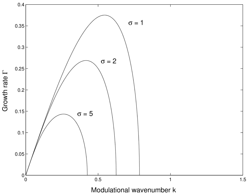
Figure 1: The growth rate $\Gamma$ as function of the wavenumber $k$ for $\sigma=1,2,5$ and Gaussian response function in the focusing case.

Now, let us consider situations where it is not assumed that the spectrum is strictly decreasing for all $k$. Then it is possible to have additional gain bands in the focusing case. We assume that

$$\phi\left(k_{2j}\right)=\phi\left(k_{2j+1}\right)=0;$$ (37)

$$\phi\left(k\right)>0\text{ for }k\in\left\langle k_{2j},k_{2j+1}\right\rangle$$ (38)

for $j=1,2,..,m-1$ where $m$ is the number of MI bands. Since $\Gamma$ $\equiv k\phi^{1/2}$ is continuous and realvalued on $\left[k_{2j},k_{2j+1}\right]$ and differentiable on $\left\langle k_{2j},k_{2j+1}\right\rangle,$ it follows from Rolles theorem that there is at least one $k_{cr}^{\left(j\right)}\in\left\langle k_{2j},k_{2j+1}\right\rangle$ such that $\Gamma^{\prime}(k_{cr}^{(j)})=0$. If, in addition

$$\phi^{\prime}(k_{2j})>0,\;\;\;\phi^{\prime}(k_{2j+1})<0,$$ (39)

we find the following limits

$$\lim_{\;\;\;\;k\rightarrow k_{2j}^{+}}\Gamma^{\prime}(k)=+\infty,\;\;\;\lim_{\;\;\;\;\;\;\;\;k\rightarrow k_{2j+1}^{-}}\Gamma^{\prime}(k)=-\infty.$$

Now, if the condition (31) is satisfied, then $k_{cr}^{\left(j\right)}=k_{\max}^{\left(j\right)}$ is a unique. Hence we have a unique maximum growth rate for this wavenumber band as well.

As an example we consider the square pulse function

$$R\left(x\right)=\frac{1}{\sigma}\Phi\left(\frac{x}{\sigma}\right);\text{ }\Phi\left(\zeta\right)=\left\{\begin{array}[]{c}\frac{1}{2};\text{ }\left|\zeta\right|\leq 1\\ 0;\text{ }\left|\zeta\right|>1\end{array}\right.;$$ (40)

whose Fourier - transform is given by

$$\widehat{R}(k)=\widehat{\Phi}(\sigma k)=\frac{\sin(k\sigma)}{k\sigma}.$$ (41)

For small and moderate values of the width $\sigma$ we only have one fundamental MI gain band. The bifurcation equation (24) reads

$$\tan(z)=z/3$$ (42)

in this case, and by means of (25) with $\widehat{\Phi}(z)>0$ ($\Leftrightarrow\sin(z)>0$), we find the critical values $\sigma_{c}.$ Moreover, one finds that $\phi^{\prime\prime}=-z^{2}-6$, from which it follows that new MI bands are excited at the bifurcation points. The table below summarizes the findings for the lowest order excitations.

$$\sigma_{c,1}=21.03$$ The second MI band is excited

The third MI band is excited

(43)

A simple computation based on (31) now reveals that each MI band has a maximum growth rate. Finally, since $\widehat{\Phi}$ of the square response function is a monotonically decreasing function on an interval containing $[0,k_{1}]$ for all values of $\sigma$, we conclude by appealing to (33) and (34) that an increase in the width $\sigma$ decreases both the fundamental band and the maximum growth rate. The expression (34) (with $k_{1}$ replaced with $k_{i}$, $(i=2j,2j+1))$ and (37)-(39) show that the higher order MI gain bands move towards lower wavenumbers as the width $\sigma$ increases. Fig. 2 summarizes these features graphically, and the results are consistent with the findings in [22].

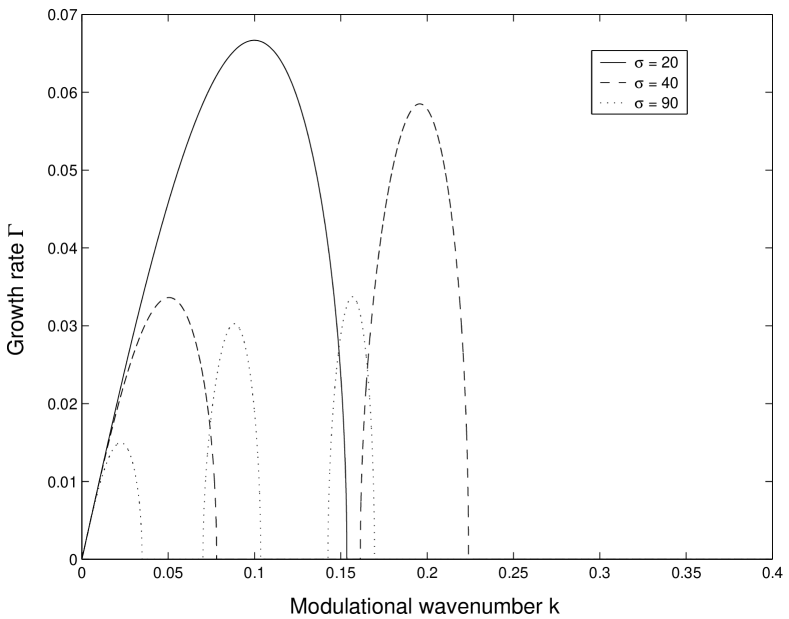
Figure 2: The growth rate $\Gamma$ as function of the wavenumber $k$ for $\sigma=20,40,90$ and the square response function in the focusing case.

II.2 The defocusing case (s=-1)

The function $\phi$ given by

$$\phi\equiv-\widehat{\Phi}\left(\sigma k\right)-k^{2};$$ (44)

in the defocusing case. Here the number of zeros of $\phi$, denoted by $N$, is even, i.e. $N=2m$ $\left(m=0,1,2,..\right)$ and there are $m$ MI bands. We observe from the list of properties of the spectrum $\widehat{\Phi}\left(\sigma k\right)$ that MI can only exist in the high wavenumber regime, as opposed to the focusing case. Notice that the case $m=0$ corresponds to the situation where $\phi\left(k\right)<0$ for all $k\geq 0$ which means modulational stability.

A typical situation revealing stability occurs when $\widehat{\Phi}(\sigma k)\geq 0$ for all $k\geq 0$, irrespective of the value of $\sigma$. The spectrum of the Gaussian (36) satisfies this property. The same holds true for the exponential response function

$$R(x)=\frac{1}{\sigma}\Phi\left(\frac{x}{\sigma}\right);\;\;\;\Phi(\zeta)=\frac{1}{2}\exp(-|\zeta|)$$ (45)

for which the Fourier - transform is given by

$$\widehat{R}(k)=\widehat{\Phi}(\sigma k)=\frac{1}{1+\sigma^{2}k^{2}}.$$ (46)

When $\widehat{\Phi}(k)$ changes sign, the picture is somewhat more complicated. First of all, we will still have stability if $\widehat{\Phi}(\sigma k)<0$ for all $k$ provided the control parameter $\sigma$ is below certain threshold $\sigma_{c}$. The threshold value $\sigma_{c}$ and the corresponding value of $k$ can be found by requiring the bifurcation condition (23) to be fulfilled. Secondly, if $\sigma$ belongs to the complementary regime, i.e., $\sigma>\sigma_{c}$ we have $\widehat{\Phi}(\sigma k)\geq 0$ for certain wavenumber intervals, and hence we may have one or more MI gain bands, whose growth rate $\Gamma$ is given by (27) and (44). Even in this case one can prove the existence of a unique maximum growth rate within each unstable band in the same way as in the focusing case.

Again we use the square pulse function (40) - (41) as an example. The bifurcation problem is solved by means of (42) - (25) with $s=-1$ and hence the extra constraint that $\sin\left(z\right)<0.$ Here we also find that $\phi^{\prime\prime}=-z^{2}-6<0$, which means that new MI bands are excited through the bifurcation process. The table below displays the bifurcation values of $\sigma$ for the lowest order excitations.

$$\sigma_{c,1}=9.146$$ The first MI band is excited

The second MI band is excited

The third MI band isexcited

(47)

The number of MI bands increases when the width increases. By (31) each MI band has a maximum growth rate. Finally, by using the expression for the velocity of the zeros $k_{2j-1}$ and $k_{2j}$ of $\phi$ $(j=1,2,..,m)$ in the defocusing case

$$\frac{dk_{i}}{d\sigma}=\frac{\widehat{\Phi}^{\prime}\left(\sigma k_{i}\right)k_{i}}{-\widehat{\Phi}^{\prime}\left(\sigma k_{i}\right)\sigma-2k_{i}};\text{ }i=2j-1,2j$$ (48)

and (37) - (39) with $\phi$ given as (44) and $k_{2j}$ and $k_{2j+1\text{ }}$replaced with $k_{2j-1}$and $k_{2j},$respectively, it can be shown in a the same way as in the focusing case that $\frac{dk_{i}}{d\sigma}<0$ and hence the MI bands move to the low wavenumber regimes as the width increases. The latter analytical result is also in accordance with the numerical results obtained in [22]. In Fig.3. the MI result for the square pulse (40) in the defocusing case is displayed.

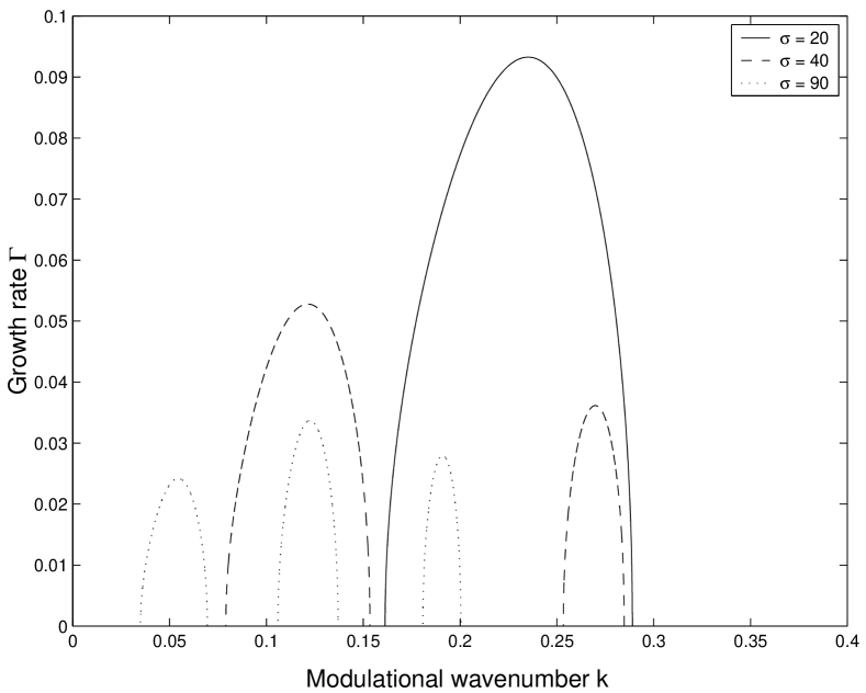
Figure 3: The growth rate $\Gamma$ as function of the wavenumber $k$ for $\sigma=20,40,90$ for the square response function in the defocusing case.

III Generalized response functions

Now, let us consider a localized response function $R(x)$ which can be written as a convex combination of $N$ response functions $R_{n}\left(x\right)$ whose properties are known i.e. the weighted mean

$$R(x)=\sum_{n=1}^{M}f_{n}R_{n}\left(x\right)\text{ , }n=1,2,3,...,M;$$ (49)

where

$$\sum_{n=1}^{M}f_{n}=1\text{ , \ }0\leq f_{n}\leq 1\text{ , }\int_{-\infty}^{\infty}R_{n}\left(x\right)dx=1;$$ (50)

and $R_{n}\left(x\right)$ is parametrized by a typical lengthscale $\sigma_{n}$, i.e. $R_{n}\left(x\right)=\sigma_{n}^{-1}\Phi_{n}\left(\frac{x}{\sigma_{n}}\right)$ with $\Phi_{n}$ as the scaling functions. From now on we refer to the functions $R_{n}\left(x\right)$ as ”building blocks”.

The corresponding spectrum $\widehat{R}\left(k\right)$ appears as a convex combination of $\widehat{R}_{n}\left(k\right)$

$$\widehat{R}\left(k\right)=\sum_{n=1}^{M}f_{n}\widehat{R}_{n}\left(k\right)=\sum_{n=1}^{M}f_{n}\widehat{\Phi}_{n}\left(\sigma_{n}k\right);$$ (51)

where $\widehat{\Phi}_{n}$ is the spectrum of the scaling function $\Phi_{n}.$ Moreover, we find in accordance with (4) that

$$\int_{-\infty}^{\infty}x^{2}R_{n}\left(x\right)dx\sim\sigma_{n}^{2};$$ (52)

A typical lengthscale $\sigma$ of the composite response function $R\left(x\right)$ can be defined

$$\sigma^{2}=\sum_{n=1}^{N}f_{n}\sigma_{n}^{2};$$ (53)

It is straightforward to show that the dispersion relation on normalized form can be expressed as

$$\lambda^{2}/\lambda_{0}^{2}=k^{2}\phi_{conv};\text{ }$$ (54)

where

$$\phi_{conv}\equiv s\sum_{n=1}^{M}f_{n}\widehat{\Phi}_{n}\left(\sigma_{n}k\right)-k^{2};$$ (55)

which is a generalization of the dispersion relation (19). Here $\lambda_{0}$ and $k$ are given as (20) and (21), respectively, while $\sigma_{n}$ is the redefined width of the response function:

$$2\sqrt{\rho_{0}}\sigma_{n}\rightarrow\sigma_{n};$$ (56)

Now, if the transversality condition $\phi_{conv}^{\prime}\neq 0$ is satisfied on points where  $\phi_{conv}=0,$ there are a finite union of disjoint, bounded and closed subintervals of the positive $k$ axis, for which $\phi_{conv}\geq 0.$ This means that the MI is of finite bandwidth type in this case as well. In each gain band the normalized growth rate $\Gamma$ is given as

$$\Gamma\equiv\left|{\cal Re}\left(\lambda\right)\right|/\lambda_{0}=\left|k\right|\phi_{conv}^{1/2};$$ (57)

In (54) - (57) there are $2M-1$ control parameters, namely the $M$ width parameters $\sigma_{1},\sigma_{2},...,\sigma_{M}$ and the $M-1$ weight parameters $f_{1},f_{2},...,f_{M-1}$. To summarize, the stability properties depend on the weight $f_{n}$ of each Fourier - transform $\widehat{\Phi}_{n}$ and length scale $\sigma_{n}$ .

Let us consider some special cases. Assume that the Fourier transforms $\widehat{R}_{n}(k)$ of all the building block functions $R_{n}(x)$ are monotonically decreasing positive functions, such as the exponential and Gaussian response functions. The sum $\sum_{n=1}^{M}f_{n}\widehat{\Phi}_{n}(\sigma_{n}kt)$ will now be a decreasing and positive function of $k$. In the defocusing case $(s=-1)$ we will have modulational stability in this case, while we get MI with one gain band about $k=0$ in the focusing case ($s$=1), which has a unique maximum growth rate. In Fig. 4. we display this phenomenon for the case when the total response function is a sum of a Gaussian and an exponential response function.

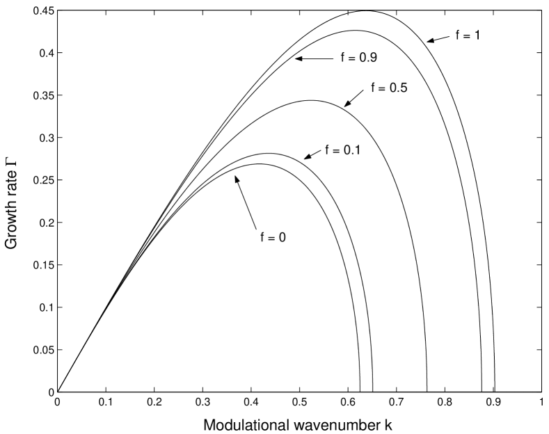
Figure 4: Growth rate $\Gamma$ versus wavenumber $k$ for a convex combination of a Gaussian response function with weight factor $f_{g}=f$ and width $\sigma_{g}$=1 and an exponential response function with weight factor $f_{e}=1-f$ and width $\sigma_{e}$=2 for different values of $f$.

In Fig. 5 we show what happens for a focusing nonlinearity when the response function is a 3-component combination of a Gaussian, an exponential, and a square response function. In Fig. 5 two MI gain bands are revealed. A typical feature of the fundamental band is that the growth rate exhibits a more complex behavior with several local extrema, as opposed to the single-maximum generic situation defined by (31).

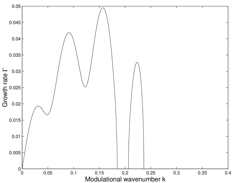
Figure 5: Growth rate $\Gamma$ versus wavenumber $k$ for a convex combination of a Gaussian (width $\sigma_{g}$=10), an exponential (width $\sigma_{e}$=20), and a square response function (width $\sigma_{sq}$=90) in the focusing case. The corresponding weight factors are $f_{g}$=0.1, $f_{e}$=0.3, and $f_{sq}$=0.6.

IV Conclusion

The linear stage of the MI for the nonlocal NLS equation is conveniently studied in terms of the spectrum of the response function. From the dispersion relation (17) it appears that the crucial point in this discussion is the location of the spectrum of the response function relative to the parabola in $k$-space. The following features complement and extend the results obtained in [22]:

• The MI is of the finite bandwidth type. It consists of a finite number of well-separated gain bands. Moreover, it is possible to predict the occurrence of excitation, vanishing, coalescence and separation of MI bands.

• For a large class of response functions, each MI band has a unique maximum growth rate. This property holds true for the Gaussian, the exponential and the square response functions. It resembles the structure of the MI bands in the focusing local NLS equation.

• In the focusing case we always find at least one MI gain band centered about $k=0$. It is verified analytically that the width of this MI band, as well as the corresponding growth rate, decreases when increasing the width of the response function, provided the spectrum of the response function is decreasing in this MI band. Furthermore, additional MI bands are excited at higher wavenumbers when the width parameter exceeds a certain threshold, i.e. when the nonlinearity becomes sufficiently nonlocal. The latter phenomenon is a unique feature of the nonlocal nonlinearity and has no equivalent in the local case and the weakly nonlocal limit.

• In the defocusing case we can either have stability or MI of the finite bandwidth type. The latter situation can only occur in the high wavenumber regime, and only if the width of the response function exceeds a certain threshold, i.e. when the nonlinearity becomes sufficiently nonlocal.

• In both the focusing and defocusing case the higher order MI bands move towards lower wavenumbers as the width of the response function increases. In the limit of strong nonlocality the MI bands vanish completely. This result agrees with the fact the strongly nonlocal limit of the NLS model (1) is a linear model.

• It is possible to study MI for more complicated multiscale scenarios where the response functions decompose into a weighted mean of ”building blocks”, where each ”building block” has a characterized width. In this case we get a richer repertory of response functions to deal with. This aims at showing that the results we have obtained represents generic features of the MI of the nonlocal NLS with general symmetric, positive response functions.

This work was supported by the Danish Technical Research Council (STVF - Talent Grant 5600-00-0355), the Danish Natural Sciences Foundation (SNF - grant 9903273), and the Graduate School in Nonlinear Science (The Danish Research Academy).

References

- [1] T.B. Benjamin and J.E. Feir, J. Fluid. Mech. 27, 417 (1967).
- [2] A. Hasegawa, Plasma instabilities and Nonlinear Effects (Springer-Verlag, Heidelberg, 1975).
- [3] L.A. Ostrovskii, Sov. Phys. JETP 24, 797 (1967).
- [4] V.I. Bespalov and V.I. Talanov, JETP Lett. 3, 307 (1966); V.I. Karpman, JETP Lett. 6, 277 (1967).
- [5] Yu.S. Kivshar and M. Peyrard, ”Modulational instabilities in discrete latices”, Phys. Rev. A46, 3198 (1992).
- [6] P.D. Miller and O. Bang, ”Macroscopic dynamics in quadratic nonlinear lattices”, Phys. Rev. E 57, 6038-6049 (1998).
- [7] S. Trillo, S. Wabnitz, G.I. Stegeman, and E.M. Wright, ”Parametric amplification and modulational instabilities in dispersive nonlinear directional couplers with relaxing nonlinearity”, J. Opt. Soc. Am. B6, 889-900 (1989).
- [8] M.J. Potasek, Opt. Lett. 12, 921 (1987)
- [9] Yu.S. Kivshar, D. Anderson, and M. Lisak, Phys. Scripta 48 679 (1993).
- [10] M. Soljacic, M. Segev, T. Coskun, D. Christodoulides, and A. Vishwanath, Phys. Rev. Lett.84, 467 (2000).
- [11] J. Wyller, ”Nonlinear wavefields in optical fibres with finite time response and amplification effects”, Physica D (to appear).
- [12] J.P. Gordon, R.C. Leite, R.S. Moore, S.P. Porto, and J.R. Whinnery, J. Appl. Phys. 36, 3 (1965).
- [13] S. Akhmanov, D.P. Krindach, A.V. Migulin, A.P. Sukhorukov, and R.V. Khokhlov, IEEE J. Quant. Electron. QE-4, 568 (1968).
- [14] M. Horovitz, R. Daisy, O. Werner, and B. Fischer, Opt. Lett. 17, 475 (1992).
- [15] D. Suter and T. Blasberg, ”Stabilization of transverse solitary waves by a nonlocal response of the nonlinear medium”, Phys. Rev. A48, 4583 (1993).
- [16] M.V. Porkolab and M.V. Goldman, ”Upper-hybrid solitons and oscillating-two-stream instabilities”, Phys. Fluids 19, 872 (1976).
- [17] A.G. Litvak and A.M. Sergeev, JETP Lett. 27, 517 (1978).
- [18] T.A. Davydova and A.I. Fishchuk, ”Upper hybrid nonlinear wave structures”, Ukr. J. Phys. 40, 487 (1995).
- [19] A.G. Litvak, V.A. Mironov, G.M. Fraiman, and A.D. Yunakovskii, ”Thermal self-effect of wave beams in a plasma with a nonlocal nonlinearity”, Sov. J. Plasma Phys. 1, 31 (1975).
- [20] H.L. Pecseli and J.J. Rasmussen, ”Nonlinear electron waves in strongly magnetized plasmas”, Plasma Phys. 22, 421 (1980).
- [21] F. Dalfovo, S. Giorgini, L.P. Pitaevskii, and S. Stringari, K. Goral, and K. Rzazewski, Phys. Rev. A61 051601R (2000); Rev. Mod. Phys. 71, 463 (1999); V.M. Perez-Garcia, V.V. Konotop, and J.J. Garcia-Ripoll, Phys. Rev. E 62, 4300 (2000).
- [22] W. Krolikowski, O. Bang, J.J. Rasmussen, and J. Wyller. ”Modulational instability in nonlocal nonlinear Kerr media”, Phys. Rev. E (to appear).
- [23] A. Parola, L. Salanich, and L. Reatto, ”Structure and stability of bosonic clouds: Alkali-metal atoms with negative scattering length”, Phys. Rev. A57, R3180 (1998).
- [24] X. Wang, D. W.Brown, K. Lindenberg, and B.J. West, ”Alternative formulation of Davydov’s theory of energy transport in biomolecular systems”, Phys. Rev. A37, 3557 (1988).
- [25] A. Nakamura, J. Phys. Soc. Japan 42, 1824 (1977).
- [26] W. Krolikowski and O. Bang, ”Solitons in nonlocal nonlinear media: Exact solutions”, Phys. Rev. E 63, 016610 (2001).
- [27] A. Snyder and J. Mitchell, ”Accessible solitons”, Science 276, 1538 (1997).
- [28] G.B. Folland, Real analysis. Modern Techniques and Their Applications. p. 241. John Wiley & Sons. ISBN 0471-80958-6. 1984.