Occurrence of periodic Lamé functions

at bifurcations in chaotic Hamiltonian systems

M Brack¹, M Mehta¹ and K Tanaka^1,2

¹Institute for Theoretical Physics, University of Regensburg, D-93040 Regensburg, Germany

²Dept. of Physics, University of Saskatchewan, Saskatoon, SK, Canada S7N5E2

Abstract

We investigate cascades of isochronous pitchfork bifurcations of straight-line librating orbits in some two-dimensional Hamiltonian systems with mixed phase space. We show that the new bifurcated orbits, which are responsible for the onset of chaos, are given analytically by the periodic solutions of the Lamé equation as classified in 1940 by Ince. In Hamiltonians with C_2v symmetry, they occur alternatingly as Lamé functions of period 2K and 4K, respectively, where 4K is the period of the Jacobi elliptic function appearing in the Lamé equation. We also show that the two pairs of orbits created at period-doubling bifurcations of island-chain type are given by two different linear combinations of algebraic Lamé functions with period 8K.

1 Introduction

One of the well-established routes to chaos in maps is the so-called Feigenbaum scenario [2] which consists in a cascade of successive period-doubling bifurcations of pitchfork type. They were first discussed for the 1-dimensional logistic map by Feigenbaum [2] and then also found in the area-conserving two-dimensional Hénon map [3, 4], although the numerical scaling constants found there differ from those in the 1-dimensional case. One of us (M.B.) has recently investigated [5] similar cascades of pitchfork bifurcations occurring in 2-dimensional Hamiltonian systems with mixed dynamics, whereby the scaling constants can be determined analytically and depend on the potential parameters. In the present paper, we shall show that the new orbits born at its bifurcations are, near the bifurcations points, analytically given by periodic solutions of a linear second-order differential equation studied over 160 years ago by G. Lamé [6], and therefore called the “periodic Lamé functions” [7]. They have been classified uniquely in 1940 by Ince [8] who also derived their Fourier series expansions [9]. We find that these not only reproduce accurately the periodic orbits found numerically by solving the equations of motion at the bifurcations, but in the Hénon-Heiles [10] and similar potentials the Lamé functions can also be used to describe the evolution of the bifurcated orbits at higher energies. A particularly interesting case is the homogeneous quartic oscillator for which the Lamé functions become finite polynomials in terms of Jacobi elliptic functions. Here we can also find analytical expressions for the algebraic Lamé functions which describe the orbits created at period-doubling bifurcations of island-chain type.

2 Bifurcations of a straight-line librating orbit

We start from an autonomous two-dimensional Hamiltonian of a particle with unit mass in a smooth potential $V(x,y)$

$$H=\frac{1}{2}\left(p_{x}^{2}+p_{y}^{2}\right)+V(x,y)\,.$$ (1)

Assume that there exists a straight-line librating orbit, called A, along the $y$ axis, so that

$$x_{A}(t)\equiv 0\,,\qquad y_{A}(t)=y_{A}(t+T_{\rm A})$$ (2)

are solutions of the equations of motion and $T_{\rm A}$ is the period of the A orbit. Its stability is obtained from the stability matrix ${\rm M}_{\rm A}$ that describes the propagation of the linearized flow of a small perturbation $\delta x(t)$, $\delta p_{x}(t)=\delta\dot{x}(t)$ transverse to the orbit A:

$$\left(\begin{array}[]{r}\delta x\,(T_{\rm A})\\ \delta p_{x}\,(T_{\rm A})\end{array}\right)={\rm M}_{\rm A}\left(\begin{array}[]{r}\delta x\,(0)\\ \delta p_{x}\,(0)\end{array}\right).$$ (3)

When $-2<{\rm tr}\,{\rm M}_{\rm A}<+2$, the orbit is stable, for $|{\rm tr}\,{\rm M}_{\rm A}|>2$ it is unstable. Marginally stable orbits with ${\rm tr}\,{\rm M}_{\rm A}=+2$ occur in systems with continuous symmetries; in two dimensions this would imply integrability. We investigate here only non-integrable systems in which all orbits are isolated. Then, an orbit must undergo a bifurcation when ${\rm tr}\,{\rm M}_{\rm A}=+2$.

The elements of the stability matrix ${\rm M}_{\rm A}$ can be calculated from solutions of the linearized equation of motion in the transverse $x$ direction, which we write in the Newtonian form

$$\left.\delta{\ddot{x}}(t)+\frac{\partial^{\,2}V(x,y)}{\partial x^{2}}\right|_{x=0,y=y_{A}(t)}\delta x(t)=0\,.$$ (4)

This equation is identical to Hill’s equation [11] in its standard form [12]

$$\delta{\ddot{x}}(t)+[\lambda+Q(t)]\,\delta x(t)=0\,,$$ (5)

where $Q(t)$ is a $T_{\rm A}$ (or $T_{\rm A}/2$) periodic function whose constant Fourier component is zero. In general, the solutions of (5) are non-periodic. However, periodic solutions with period $T_{\rm A}$ (or $T_{\rm A}/2$) and multiples thereof exist for specific discrete values of $\lambda$. This happens exactly at bifurcations of the A orbit where ${\rm tr}\,{\rm M}_{\rm A}=+2$. The periodic solutions $\delta x(t)$ found at these discrete values of $\lambda$ describe the $x$ motion of the bifurcated orbits infinitely close to the bifurcation point. A special case of the Hill equation is the Lamé equation which we discuss in the following section.

3 The periodic Lamé functions

One of the standard forms of the Lamé equation reads [13]

$$\Lambda^{\prime\prime}(z)+\left[h-n(n+1)\,k^{2}\,{\rm{\rm sn}}^{2}(z,k)\right]\Lambda(z)=0\,,$$ (6)

where ${\rm sn}(z,k)$ is a Jacobi elliptic function with modulus $k$ limited by $0\leq k<1$. The real period of ${\rm sn}(z,k)$ in the variable $z$ is 4K, where

$$\hbox{\bf K}=K(k)=F\left(\frac{\pi}{2},k\right)$$ (7)

is the complete elliptic integral of the first kind with modulus $k$. We follow throughout this paper the notation of Gradshteyn and Ryzhik [14] for elliptic functions and integrals. We are interested here only in real solutions for $\Lambda(z)$ with real argument $z$. Hence $h$ and $n(n+1)$ are assumed here to be arbitrary real constants. This means that $n$ is either real, or complex with real part $-\frac{1}{2}$. There is a vast literature on the periodic solutions of Eq. (6); for an exhaustive presentation of their definition and series expansions as well as the most relevant literature, we refer to Erdélyi et al [13]. (See also [7] for literature prior to 1932.) Ince [8, 9] has introduced a unique classification and nomenclature for the four types of periodic solutions, calling them Ec${}_{n}^{m}(z)$ and Ec${}_{n}^{m}(z)$, where $n$ is the parameter appearing in (6) and $m$ an integer giving the number of zeros in the interval $0\leq z<2\hbox{\bf K}$. Following a slight redefinition by Erdélyi [15], the Ec$(z)$ are even and the Es$(z)$ are odd functions of $z-\hbox{\bf K}$, respectively. When $m$ is an even integer, the Lamé functions have the period $2\hbox{\bf K}$ in the variable $z$, which is the same as the period of ${\rm sn}^{2}(z,k)$ appearing in (6); when $m$ is odd, they have the period $4\hbox{\bf K}$. Solutions with period $2p\hbox{\bf K}$ ($p=3,4,\dots$) can also be found; we shall discuss some solutions with period $8\hbox{\bf K}$ further below. All these periodic solutions exist only for discrete eigenvalues of $h$, denoted by $a_{n}^{m}$ and $b_{n}^{m}$ for the Ec${}_{n}^{m}$ and Es${}_{n}^{m}$, respectively; there exists exactly one solution of each of the above four types of Lamé functions for each $m\geq 0$. The eigenvalues of $h$ can, in principle, be found by solving the characteristic equation obtained from an infinite continued fraction [8] which is, however, rather difficult to evaluate in the general case. In the context of our paper, they are determined by bifurcations of a linear periodic orbit and we obtain them therefore from a numerical calculation of its stability discriminant ${\rm tr}\,{\rm M}_{\rm A}$.

The Fourier expansions derived by Ince [9], with the modification by Erdélyi [15], are given in terms of the variable

$$\zeta=\frac{\pi}{2}-{\rm am}(z,k),$$ (8)

where ${\rm am}(z,k)=\arcsin[{\rm sn}(z,k)]$, and read as follows:

$${\rm Ec}_{n}^{2m}(z) = \frac{1}{2}A_{0}+\sum_{r=1}^{\infty}A_{2r}\cos(2r\zeta)\,,\qquad\qquad\qquad(\hbox{period }2\hbox{\bf K})$$ (9)

$${\rm Ec}_{n}^{2m+1}(z) = \sum_{r=0}^{\infty}A_{2r+1}\cos[(2r+1)\zeta]\,,\!\qquad\qquad\qquad(\hbox{period }4\hbox{\bf K})$$ (10)

$${\rm Es}_{n}^{2m}(z) = \sum_{r=1}^{\infty}B_{2r}\sin(2r\zeta)\,,\qquad\quad\;\qquad\qquad\qquad(\hbox{period }2\hbox{\bf K})$$ (11)

$${\rm Es}_{n}^{2m+1}(z) = \sum_{r=0}^{\infty}B_{2r+1}\sin[(2r+1)\zeta]\,,\qquad\qquad\qquad(\hbox{period }4\hbox{\bf K})$$ (12)

with $m=0,$ 1, 2, …The expansion coefficients can be calculated by two-step recurrence relations; we give them here only for the $A_{2r}$

$$\left[n(n+1)-2\right]k^{2}A_{2} = [2h-k^{2}n(n+1)]A_{0}\,,$$ (13)

$$\left[n(n+1)-(2r+2)(2r+1)\right]k^{2}A_{2r+2} = 2\!\left[2h-k^{2}n(n+1)-4r^{2}(2-k^{2})\right]A_{2r}$$ (14)

$$-\left[n(n+1)-(2r-2)(2r-1)\right]k^{2}A_{2r-2}\,,\qquad$$

(with $r=1,$ 2, 3, …) and refer to Erdélyi et al ([13], ch 15.5.1) for the other recurrence relations which look very similar.

Although the series (9) - (12) are known [9] to converge for $k<1$, they turned out to be semiconvergent in our numerical calculations for the cases with complex $n$, due to the fact that the characteristic values of $h$ were only determined approximately. We have truncated the above series at the value $r_{max}$ where the corresponding coefficient has its smallest absolute value before starting to diverge. The cut-off values $r_{max}$ were found to increase with the order $m$ of the Lamé function; their values are given in the Tables 1 and 2 in Secs. 4 and 5, respectively.

When $n$ is an integer, the Fourier series terminate at finite values of $r$. The Lamé functions then become [8] finite polynomials in the Jacobi elliptic functions ${\rm sn}(z)$, ${\rm dn}(z)$, and ${\rm cn}(z)$, and are called the “Lamé polynomials” in short. In Sec. 6 we will encounter a special case of the Lamé equation in which $h$ and $n$ are not independent, but where $h=\frac{1}{2}n(n+1)$ along with $k^{2}=\frac{1}{2}$. Then, to each integer $n$ there exists only one value of $m$. Although the lowest few polynomials of this type and their eigenvalues of $h$ are included in the tables given by Ince [8], we give below their explicit expressions which take a particularly simple form. The basic four types of solutions correspond to the four rest classes modulo 4 of the integer $n$. With $p=0,$ 1, 2, 3, we obtain the following sums which are finite since the expansion coefficients become identically zero for $r>p$:

$${\rm Ec}_{4p}^{2p}(z) = \sum_{r=0}^{p}A_{4r}\,{\rm cn}^{4r}(z)\,,\qquad\qquad\qquad\qquad\qquad(\hbox{period }2\hbox{\bf K})$$ (15)

$${\rm Ec}_{4p+1}^{2p+1}(z) = {\rm cn}(z)\sum_{r=0}^{p}C_{4r}\,{\rm cn}^{4r}(z)\,,\quad\;\;\qquad\qquad\qquad(\hbox{period }4\hbox{\bf K})$$ (16)

$${\rm Es}_{4p+2}^{2p+1}(z) = {\rm dn}(z)\,{\rm sn}(z)\sum_{r=0}^{p}D_{4r}\,{\rm cn}^{4r}(z)\,,\qquad\qquad\quad(\hbox{period }4\hbox{\bf K})$$ (17)

$${\rm Es}_{4p+3}^{2p+2}(z) = {\rm cn}(z)\,{\rm dn}(z)\,{\rm sn}(z)\sum_{r=0}^{p}B_{4r}\,{\rm cn}^{4r}(z)\,.\quad\quad\;\;\,(\hbox{period }2\hbox{\bf K})$$ (18)

The simple one-step recurrence relations for the coefficients are (with $r=0,$ 1, 2, …, $p-1$)

$$(r+1)(4r+3)\,A_{4r+4} = -[p(4p+1)-r(4r+1)]\,A_{4r}\,,$$ (19)

$$2(r+1)(4r+5)\,C_{4r+4} = -[(2p+1)(4p+1)-(2r+1)(4r+1)]\,C_{4r}\,,$$ (20)

$$2(r+1)(4r+3)\,D_{4r+4} = -[(2p+1)(4p+3)-(2r+1)(4r+3)]\,D_{4r}\,,$$ (21)

$$(r+1)(4r+5)\,B_{4r+4} = -[(p+1)(4p+3)-(r+1)(4r+3)]\,B_{4r}\,.$$ (22)

The first sixteen Lamé polynomials obtained from the above equations are given explicitly in Sec. 6 (see Table 3), with the normalization $A_{0}=B_{0}=C_{0}=D_{0}=1$.

For half-integer values of $n$, one obtains periodic Lamé functions with period $8\hbox{\bf K}$ that have algebraic forms in the Jacobi elliptic integrals and are called “algebraic Lamé functions” [9, 16]. For the special case with $k^{2}=\frac{1}{2}$ and $h=\frac{1}{2}n(n+1)$ we will encounter them in Sec. 6 at period-doubling bifurcations of island-chain type. As shown in a beautiful paper by Ince [9], there exist two linearly independent periodic solutions for $n=2p+\frac{1}{2}$ with $p=0,$ 1, 2, …

$${\rm Ec}_{2p+1/2}^{m+1/2}(z) = \sqrt{{\rm dn}(z)+{\rm cn}(z)}\,\left\{\sum_{r=0}^{p}A_{r}\,{\rm sn}^{2r}(z)+{\rm cn}(z)\,{\rm dn}(z)\sum_{r=0}^{p-1}B_{r}\,{\rm sn}^{2r}(z)\right\},$$ (23)

$${\rm Es}_{2p+1/2}^{m+1/2}(z) = \sqrt{{\rm dn}(z)-{\rm cn}(z)}\,\left\{\sum_{r=0}^{p}A_{r}\,{\rm sn}^{2r}(z)-{\rm cn}(z)\,{\rm dn}(z)\sum_{r=0}^{p-1}B_{r}\,{\rm sn}^{2r}(z)\right\},$$ (24)

where $m$ is the number of zeros in the open interval $(0,2\hbox{\bf K})$; the coefficients $A_{r}$ and $B_{r}$ are given by two coupled recurrence relations. For $k^{2}=\frac{1}{2}$, $h=\frac{1}{2}n(n+1)=2p(p+1)+\frac{3}{8}$, there is only one solution with $m=p$ for each $p$, and the recurrence relations read

$$2(2r+2)^{2}A_{r+1}+[4p(p+1)-6r(2r+1)]A_{r}-4(p-r+1)(p+r)A_{r-1}\qquad\;\;$$

$$=2(2r+2)B_{r+1}-3(2r+1)B_{r}+2rB_{r-1},$$ (25)

$$(2r+2)^{2}B_{r+1}+[2p(p+1)-3(r+1)(2r+1)]B_{r}-2(p-r)(p+r+1)B_{r-1}$$

$$=(2r+2)A_{r+1}.$$ (26)

These relations hold for $r\geq 0$ provided that coefficients with negative indices $r$ are taken to be zero. It is quite easy to see that $B_{r}=A_{r+1}=0$ for $r\geq p$, which justifies the upper limits of the sums above. The coefficient $A_{0}$ may be used for the overall normalization of both functions.

The algebraic Lamé functions (23) and (24) are even and odd functions of $z$, respectively, and related to each other by Ec${}_{2p+1/2}^{m+1/2}(z+2\hbox{\bf K})=$ Es${}_{2p+1/2}^{m+1/2}(z)$, which amounts to a sign change in front of ${\rm cn}(z)$. Erdélyi [16] showed that the linear combinations Ec${}_{2p+1/2}^{m+1/2}(z)\;+$ Es${}_{2p+1/2}^{m+1/2}(z)$ and Ec${}_{2p+1/2}^{m+1/2}(z)\;-$ Es${}_{2p+1/2}^{m+1/2}(z)$ are even and odd functions of $z-\hbox{\bf K}$, respectively, and proposed that they be used instead of the functions (23,24) introduced by Ince. However, as we shall see in Sec. 6, both pairs of independent functions are relevant in connection with period-doubling bifurcations. The Lamé functions found for $0\leq p\leq 3$ are explicitly given in Table 4 of Sec. 6.

4 The Hénon-Heiles potential

We investigate here the role of the straight-line librating orbit A in the Hénon-Heiles (HH) potential [10]. The Hamiltonian reads in scaled coordinates

$$e=6H=6\left[\frac{1}{2}\,(p_{x}^{2}+p_{y}^{2})+V_{\rm H\!H}(x,y)\right],\qquad V_{\rm H\!H}(x,y)=\frac{1}{2}\,(x^{2}+y^{2})+x^{2}y-\frac{1}{3}\,y^{3},$$ (27)

whereby the scaled energy is $e=1$ at the saddle points. The Newton equations of motion are

$$\ddot{x}+(1+2y)\,x = 0\,,$$ (28)

$$\ddot{y}+y-y^{2}+x^{2} = 0\,.$$ (29)

These equations, and therefore the classical dynamics of the HH potential, depend only on the scaled energy $e$ as a single parameter. In our numerical investigations we have solved Eqs. (28,29) and determined the periodic orbits by a Newton-Raphson iteration using their stability matrix [17].

The basic periodic orbits with shortest periods found in the HH potential have been discussed mathematically by Churchill et al [18]; an exhaustive numerical search and classification has been performed by Davies et al [19]. We focus here on the straight-line A orbit which exists along the three symmetry axes of the HH potential, one of which coincides with the $y$ axis. This orbit undergoes an infinite series of bifurcations which were studied in Ref. [5]. They form a geometric progression on the scaled energy axes $e$, cumulating at the critical energy $e=1$ where the period $T_{\rm A}$ becomes infinity and the orbit A becomes non-compact. All the orbits bifurcated from it exist, however, also at $e>1$ and stay in a bounded region of the $(x,y)$ space. Vieira and Ozorio de Almeida [20] have investigated some of these orbits at $e>1$, both numerically and semi-analytically using Moser’s converging normal forms near a harmonic saddle. In Fig. 1 we show the shapes of the orbits born at the isochronous bifurcations of orbit A, i.e., of those orbits having the same period $T_{\rm A}$ as orbit A at the bifurcation points. The subscripts of their names O_σ indicate their Maslov indices $\sigma$ needed in the context of the semiclassical periodic orbit theory [21, 22, 23]. Although we make no use of the Maslov indices in the present paper, they are a convenient means of classification of the bifurcated orbits, as will become evident from the systematics below.

All orbits shown in Fig. 1 are evaluated at the barrier energy $e=1$. In the upper part of the figure, the $x$ axis has been zoomed by a factor 0.163 from each panel to the next, in order to bring the shapes to the same scale. The orbits look practically identical in the lower 97% of their vertical range, but near the barrier ($y=1$) they make one more oscillation in the $x$ direction with each generation. In the lower part of the figure, we have zoomed also the $y$ axis by the same factor from one panel to the next and plotted the top part of each orbit, starting from $y=1$. In these blown-up

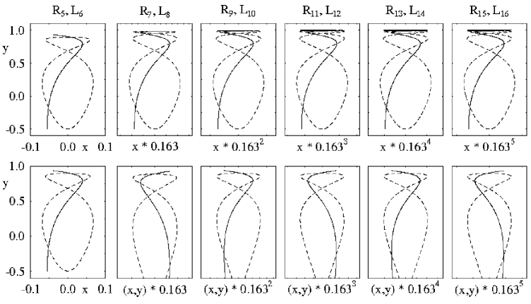
Figure 1: Orbits bifurcated from the A orbit in the HH potential, evaluated at energy $e=1$. The subscripts give their Maslov indices $\sigma$. Dashed lines: rotations R_σ, solid lines: librations L_σ (only one libration orbit is shown for each index; its partner is obtained by reflection at the vertical symmetry line containing orbit A). Top panels: successive scaling of $x$ axis from left to right with the factor 0.163. Bottom panels: successive scaling of both axes with the same factor; along the $y$ axis only the top part (starting from $y=1$) is shown.

scales, the tips of the orbits exhibit a perfect self-similarity which has been described by analytical scaling constants in Ref. [5].

In Fig. 2 we show the stability discriminant ${\rm tr\,M}$ for the orbit A (with its Maslov index $\sigma$ increasing by one unit at each bifurcation) and the orbits born at its isochronous bifurcations, plotted versus scaled energy $e$. In the lowest panel, we see the uppermost 3% of the energy scale available for the orbit A. The first bifurcation occurs at $e_{5}=0.969309$, where A₅ becomes unstable (with ${\rm tr}\,{\rm M}_{\rm A}$ $>2$) and the stable orbit R₅ is born. At $e_{6}=0.986709$, orbit A₆ becomes stable again and a new unstable orbit L₆ is born. In the middle panel, we have zoomed the uppermost 3% of the previous energy scale. Here the behavior of A repeats itself, with the new orbits R₇ and L₈ born at the next two bifurcations. Zooming with the same factor to the top panel, we see the birth of R₉ and L₁₀. This can be repeated ad infinitum: each new figure will be a replica of the previous one, with all the Maslov indices increased by two units and with ${\rm tr}\,{\rm M}_{\rm A}$ oscillating forever. This fractal behaviour is characteristic of the “Feigenbaum route to chaos” [2, 3, 4], although the present system is different from the Hénon map in that the pitchfork bifurcations seen in Fig. 2 here are isochronous due to the reflection symmetry of the HH potential around the lines on which the bifurcating orbit A is situated (see Refs. [24, 25, 26] for a discussion of the non-generic nature of the bifurcations in potentials with discrete symmetries). Also, the successive bifurcations happen here from one and the same orbit A, whereas in the standard Feigenbaum scenario one studies repeated period doubling bifurcations.

Note that the functions ${\rm tr\,M}(e)$ of the bifurcated orbits in Fig. 2 are approximately linear and intersect at $e=1$ in two points, one for the librating orbits L_σ with ${\rm tr\,M}_{\rm L}(e=1)=+8.183$ (lying outside the figure), and one for the rotating orbits R_σ with ${\rm tr\,M}_{\rm R}(e=1)=-4.183$. We shall derive this linear behaviour in the limit $e\rightarrow 1$ from an asymptotic analytical evaluation of ${\rm tr}\,{\rm M}_{\rm A}$ in a forthcoming publication [27].

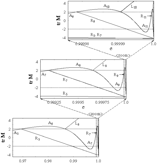
Figure 2: Trace of stability matrix M of orbit A and the orbits born at successive pitchfork bifurcations in the HH potential, plotted versus scaled energy $e$. From bottom to top: successively zoomed energy scale near $e=1$.

Presently we focus on the shapes of the orbits born at the bifurcations of A. Infinitely close to the bifurcation points, their motion in the transverse $x$ direction is given by periodic solutions of the stability equation (5). Note that this equation is identical with the full equation of motion (28) in the $x$ direction, which happens to be linear for the HH potential. The function $y_{A}(t)$ describing the A orbit can easily be found analytically [5] and is given, with the initial condition $y_{A}(0)=y_{1}$, by

$$y_{A}(t)=y_{1}+(y_{2}-y_{1})\,{\rm sn}^{2}(z,k)\,,$$ (30)

where $z$ is the scaled time variable

$$z=\sqrt{(y_{3}-y_{1})/6}\,t=at\,,$$ (31)

and $y_{i}$ ($i=1,$ 2, 3) are the roots of the cubic equation $e=6\,V_{\rm H\!H}(x=0,y)=3\,y^{2}-2\,y^{3}$. $y_{1}$ and $y_{2}$ are the turning points of the A orbit, whose period is

$$T_{\rm A}=2\sqrt{6/(y_{3}-y_{1})}\,\hbox{\bf K}=(2/a)\,\hbox{\bf K}\,.$$ (32)

The modulus of the elliptic integral is given by

$$k^{2}=(y_{2}-y_{1})/(y_{3}-y_{1})$$ (33)

and tends to unity for $e\rightarrow 1$ where $y_{2}=y_{3}$. Rewriting Eq. (28) in terms of the scaled time variable $z$, it becomes identical with the Lamé equation (6), with

$$h=6\,(1+2\,y_{1})/(y_{3}-y_{1})\,,\qquad n(n+1)=-12\quad\Leftrightarrow\quad n=-1/2\pm(i/2)\sqrt{47}.$$ (34)

$e^{\star}_{\sigma}$	Oσ	$x_{\sigma}(t)$	$r_{max}$	$P$	$e_{\sigma}$	Oσ	$x_{\sigma}(t)$	$r_{max}$	$P$
0.811715516	F9	Ec${}_{n}^{3}(at)$	13	4K	0.9693090904	R5	Es${}_{n}^{4}(at)$	20	2K
0.915214692	F10	Es${}_{n}^{3}(at)$	12	4K	0.9867092353	L6	Ec${}_{n}^{4}(at)$	26	2K
0.995013	F13	Ec${}_{n}^{5}(at)$	25	4K	0.9991878410	R7	Es${}_{n}^{6}(at)$	39	2K
0.99784905	F14	Es${}_{n}^{5}(at)$	30	4K	0.9996498	L8	Ec${}_{n}^{6}(at)$	40	2K
0.99986763	F17	Ec${}_{n}^{7}(at)$	53	4K	0.999978390	R9	Es${}_{n}^{8}(at)$	67	2K
0.99994292	F18	Es${}_{n}^{7}(at)$	62	4K	0.9999906955	L10	Ec${}_{n}^{8}(at)$	104	2K
0.999996482	F21	Ec${}_{n}^{9}(at)$	123	4K	0.999999424	R11	Es${}_{n}^{10}(at)$	152	2K
0.999998483	F22	Es${}_{n}^{9}(at)$	162	4K	0.9999997525	L12	Ec${}_{n}^{10}(at)$	211	2K
0.9999999065	F25	Ec${}_{n}^{11}(at)$	290	4K	0.99999998475	R13	Es${}_{n}^{12}(at)$	450	2K
0.9999999593	F26	Es${}_{n}^{11}(at)$	276	4K	0.99999999343	L14	Ec${}_{n}^{12}(at)$	517	2K
0.999999997514	F29	Ec${}_{n}^{13}(at)$	765	4K	0.9999999996046	R15	Es${}_{n}^{14}(at)$	757	2K
0.999999998928	F30	Es${}_{n}^{13}(at)$	890	4K	0.9999999998249	L16	Ec${}_{n}^{14}(at)$	1203	2K

Table 1:  Bifurcation energies $e_{\sigma}$, $e^{\star}_{\sigma}$ of the A orbit in the Hénon-Heiles (HH) potential, names O_σ of the bifurcated orbits, Lamé functions of their motion $x_{\sigma}(t)$; cut-off order $r_{max}$ of the Fourier expansion, and period $P$ of the Lamé functions. The constant $a$ is given in (31). Right part: isochronous bifurcations; left part: period-doubling bifurcations.

Note that $h$ depends on the energy $e$. Hence, the discrete eigenvalues $h=a_{n}^{m},$ $b_{n}^{m}$ can be directly related to the bifurcation energies $e_{\sigma}$ of the orbit A, and the corresponding Lamé functions Ec${}_{n}^{m}(z)$ and Es${}_{n}^{m}(z)$ to the motion $x(z)=x(at)$ of the new periodic orbits O_σ born at the bifurcations. In Table 1 we give the bifurcation energies $e_{\sigma}$ obtained from the numerical computation of ${\rm tr}\,{\rm M}_{\rm A}$, the names O_σ of the bifurcated orbits, and the corresponding Lamé functions with their periods in the variable $z=at$ given in (31). We also give the values $r_{max}$ at which the Fourier series (9) – (12) have been truncated. The right part of the table contains the lowest isochronous bifurcations seen in Fig. 2 and the bifurcated orbits shown in Fig. 1; their Lamé functions all have the period 2K.

The left part of Table 1 contains the lowest non-trivial period-doubling bifurcations (where ${\rm tr}\,{\rm M}_{\rm A}=-2$), which are also of pitchfork type, and the names of the orbits born thereby. Their Lamé functions have the period 4K. To avoid ambiguities, we denote their bifurcation energies by $e^{\star}_{\sigma}$. The period-doubling bifurcations of new orbits with the Maslov indices 11, 12, 15, 16, etc., are trivial in the sense that they just involve the second iterates of orbit A and of the bifurcated orbits R₅, L₆, R₇, L₈, etc. The shapes of the first six non-trivial new orbits born at these bifurcations are shown in Fig. 3; they have similar scaling properties as those shown in Fig. 1.

Figure 3: The periodic orbits born at the six lowest period-doubling bifurcations of orbit A in the Hénon-Heiles potential. The $x$ axis has been scaled like in Fig. 1.

Mathematically speaking, the periodic solutions for $x_{\sigma}(t)$ in the form of the Lamé functions exist only at the bifurcation energies $e_{\sigma}$. However, the bifurcated orbits exist for all $e\geq e_{\sigma}$. As long as the amplitude of their $x$ motion remains small, it must be given by the Lamé equation (6) with the constants appearing in (34). But this equation has only periodic solutions when $h$ has an eigenvalue corresponding to a bifurcation energy $e_{\sigma}$. Therefore, the bifurcated orbits must keep their $y$ motion “frozen” at $y(t)=y_{A}(t)$ with the parameters corresponding to $e_{\sigma}$. Consequently, they also keep their periods at the bifurcation values. This has been confirmed numerically, as noticed already in [5], to hold up to $e=1$ and even beyond. Within the same small-amplitude limit of the $x$ motion, the energy of the $y$ motion is frozen at its value $e_{\sigma}$, and the excess energy $e-e_{\sigma}$ is consumed to rescale the amplitude of $x(t)$. In other words, we can determine the normalization of the Lamé function $x_{\sigma}(t)$ of each bifurcated orbit by exploiting the energy conservation. This is most easily done at the time $t_{0}=T_{A}/2$ where $y(t)$ has its maximum value, i.e., $y(t_{0})=y_{2}$, ${\dot{y}}(t_{0})=0$, and around which we know the symmetry of the Lamé functions. For the even functions Ec${}_{n}^{m}$ we have ${\dot{x}}_{\sigma}(t_{0})=0$, and $x_{\sigma}(t_{0})$ is, with (27), found to be

$$x_{\sigma}(t_{0})=\sqrt{(e-e_{\sigma})/3(1+2y_{2})}\,.$$ (35)

For the odd functions Es${}_{n}^{m}$ we have $x_{\sigma}(t_{0})=0$, and their slopes at $t_{0}$ are given by

$${\dot{x}}_{\sigma}(t_{0})=\sqrt{(e-e_{\sigma})/3}\,.$$ (36)

In this way we can not only normalize the Lamé functions near the bifurcation points, but also predict their evolution at higher energies.

In Figs. 4 - 7 show some of the periodic orbits obtained numerically from solving the equations of motion (28,29) at $e=1$ by solid lines, and compare them to those predicted in the frozen-$y$-motion approximation, using $y(t)=y_{A}(t)$ (given at their bifurcation energies $e_{\sigma}$ or $e^{\star}_{\sigma}$) and using for $x(t)$ the Lamé functions according to Table 1, scaled as explained above. We see that in all cases, even for the lowest bifurcations, the new orbits keep their $y$ motion acquired at their bifurcation energies, up to $e=1$, indeed: the two curves $y(t)$ and $y_{A}(t)$ can hardly be distinguished. As a consequence,

Figure 4: Orbit R₅ in the HH potential at $e=1$. Left panels: $y(t)$ and $x(t)$ versus time $t$ (in units of 0.01); Right panel: orbit in the $(x,y)$ plane. Solid lines: numerical results obtained by solving Eqs. (28,29). Dashed lines: $y(t)$ given by $y_{A}(t)$ in (30) at the bifurcation energy $e_{5}$, and $x(t)$ given by the Lamé function according to Table 1, scaled as described in the text.

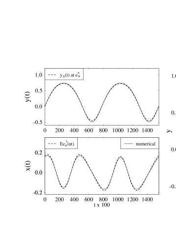
Figure 5: Same as Fig. 4 for the orbit F₉. Note that this orbit has twice the period of orbit A at $e^{\star}_{9}$ and is given by the Lamé function Ec${}_{n}^{3}(at)$ with period 4K and $m=3$ zeros in the interval $0\leq at<2\hbox{\bf K}$.

we can expect the functions $x(t)$ to be well described by the appropriate Lamé functions. This is, indeed, the case if the latter are correctly scaled. As we see, the normalization predicted by (35,36) is the better, the closer the bifurcation energy $e_{\sigma}$ comes to the saddle-point energy $e=1$. A rigorous justification of the frozen-$y$-motion approximation will be presented elsewhere [27].

We point out that all orbits born at the isochronous pitchfork bifurcations in the HH system are given by Lamé functions with period 2K, since the orbit A is given by $y_{A}(t)$ (30) and hence has the same period as the function appearing in the Lamé equation. The Lamé functions with period 4K must therefore correspond to orbits born at period-doubling bifurcations (see Table 1 and Fig. 5).

Figure 6: Same as Fig. 4 for the orbit L₈.

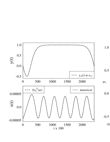
Figure 7: Same as Fig. 4 for the orbit R₁₃. Note that $x(t)$ is harmonic over a long time while $y$ is close to the saddle ($y\simeq 1$); the period of this harmonic oscillation is $\omega_{\perp}=2\pi/\sqrt{3}$, as shown in Ref. [5] and also obtained from an asymptotic expansion of the Lamé functions [27].

Note also that according to bifurcation theory [24, 25, 26, 28], two degenerate periodic orbits should be born at each isochronous pitchfork bifurcation. The librating orbits L_σ come, indeed, in pairs that are symmetric to the $y$ axis, whereas the rotating orbits R_σ can be run through in two opposite directions. Each of these pairs of orbits are, however, described by one and the same Lamé function for $x(t)$ which is invariant under the corresponding symmetry operation. This is in agreement with a theorem, proved by Ince [9], that there cannot exist two linearly independent periodic solutions of the Lamé equation to the same characteristic value of $h$. An exception of this theorem is given by transcendental and algebraic Lamé functions with integer or half-integer values of $n$ (see Sec. 6 for an example).

We finally note that in the figures 4 - 7, the time scales are not always normalized such that $t=0$ corresponds to $y(0)=y_{1}$, as assumed in Eq. (30), but obtained rather randomly due to the way in which the periodic orbits where searched and found numerically. However, if we shift the time origin to $t^{\prime}=0$ according to (30), all figures illustrate how the Lamé functions Ec${}_{n}^{m}(z)$ are even and the Es${}_{n}^{m}(z)$ odd, according to their definition [8, 16], around $t^{\prime}=\hbox{\bf K}/a$ where $y(t^{\prime})$ has its maximum. This demonstrates that the association of Lamé functions to bifurcated orbits allows one to understand (or predict) their symmetries.

5 The quartic Hénon-Heiles potential

We next investigate the quartic Hénon-Heiles (H4) potential [29, 30] with the scaled Hamiltonian

$$e=4H=4\left[\frac{1}{2}\,(p_{x}^{2}+p_{y}^{2})+V_{\rm H4}(x,y)\right],\quad V_{\rm H4}(x,y)=\frac{1}{2}\,(x^{2}+y^{2})-\frac{1}{4}\,(x^{4}+y^{4})+\frac{3}{2}\,x^{2}y^{2},$$ (37)

which is similar to the HH potential but has four saddles at the scaled energy $e=1$; it has reflection symmetry at both coordinate axes and both diagonals. It contains straight-line librating orbits along all four symmetry lines; two of them, which we call again orbits A, oscillate between the two saddles lying on the coordinate axes. To be specific, we choose again the A orbit along the $y$ axis. It has the same behaviour as the A orbit in the HH potential, but it approaches a saddle at both ends. Its motion is, for $y_{A}(0)=0$, given by

$$y_{A}(t)=y_{1}\,{\rm sn}(at,k)\,,\qquad a=y_{2}/\sqrt{2}\,,\qquad k=y_{1}/y_{2}\,,$$ (38)

and its period is

$$T_{\rm A}=4\sqrt{2}\hbox{\bf K}/y_{2}=4\hbox{\bf K}/a\,.$$ (39)

Hereby $\pm y_{1}$ and $\pm y_{2}$ are the solutions of $e=4V_{\rm H4}(x=0,y)=2\,y^{2}-y^{4}$, i.e.,

$$y_{1}=\sqrt{1-\sqrt{1-e}}\,,\qquad y_{2}=\sqrt{1+\sqrt{1-e}}\,,$$ (40)

and $\pm y_{1}$ are the turning points of the orbit.

The linearized equation of motion in the $x$ direction, which decides about the stability of the orbit A, is for the H4 potential

$${\ddot{x}}(t)+[1+3y^{2}(t)]\,x(t)=0\,,$$ (41)

neglecting here explicitly a term of order $x^{3}$. Inserting the solution for $y_{A}(t)$ in (38) and transforming to the scaled time variable $z=at$ leads again to the Lamé equation (6) with

$$h=2/y_{2}^{2}\,,\qquad n(n+1)=-6\quad\Leftrightarrow\quad n=-1/2\pm(i/2)\sqrt{23}\,.$$ (42)

Compared to the HH potential, we have now a new situation which is a consequence of the higher symmetry of the H4 potential: the periodic function ${\rm sn}^{2}(z,k)$ appearing in the stability equation has half the period, namely 2K, of that of the orbit A itself (39). Therefore, all its periodic solutions with period $2\hbox{\bf K}$, corresponding to Lamé functions with an even number $m$ of zeros, also have the period $T_{\rm A}/2$ at the bifurcations. The solutions involving the Lamé functions with odd $m$ share their periods $4\hbox{\bf K}=aT_{\rm A}$ with that of the A orbit.

The systematics of the isochronous bifurcations of the A orbit for increasing bifurcation energies $e_{\sigma}$ is given in Table 2. The new orbits appear with $m=2,$ 3, 4, …, with alternatingly odd and even Lamé functions. Like in the HH case, the Ec${}_{n}^{m}$ correspond to librations L_σ and the Es${}_{n}^{m}$ to rotations R_σ. They appear alternatingly as 2K and 4K periodic functions. The orbits given in the left part of the table are born stable and remain stable up to $e>1$, whereas those in the right part are unstable at all energies.

$e_{\sigma}$	Oσ	$x(t)$	$r_{max}$	$P$	$e_{\sigma}$	Oσ	$x(t)$	$r_{max}$	$P$
0.8561220	R5	Es${}_{n}^{2}(at)$	7	2K	0.8967139	L6	Ec${}_{n}^{2}(at)$	9	2K
0.9841765	L7	Ec${}_{n}^{3}(at)$	11	4K	0.9889128	R8	Es${}_{n}^{3}(at)$	12	4K
0.9982845	R9	Es${}_{n}^{4}(at)$	18	2K	0.9988004	L10	Ec${}_{n}^{4}(at)$	22	2K
0.9998140	L11	Ec${}_{n}^{5}(at)$	29	4K	0.99986995	R12	Es${}_{n}^{5}(at)$	32	4K
0.99997983	R13	Es${}_{n}^{6}(at)$	46	2K	0.99998590	L14	Ec${}_{n}^{6}(at)$	48	2K
0.999997812	L15	Ec${}_{n}^{7}(at)$	77	4K	0.9999984705	R16	Es${}_{n}^{7}(at)$	98	4K
0.9999997627	R17	Es${}_{n}^{8}(at)$	117	2K	0.9999998340	L18	Ec${}_{n}^{8}(at)$	134	2K
0.9999999742	L19	Ec${}_{n}^{9}(at)$	194	4K	0.9999999820	R20	Es${}_{n}^{9}(at)$	236	4K

Table 2:  The same as in Table 1, but only for the isochronous bifurcations of the A orbit in the quartic Hénon-Heiles (H4) potential. Note the alternating appearance of 2K and 4K periodic Lamé functions with increasing bifurcation energy $e_{\sigma}$. The constant $a$ is given in Eq. (38). Orbits appearing on the left side are stable up to $e>1$, those on the right side are unstable at all energies.

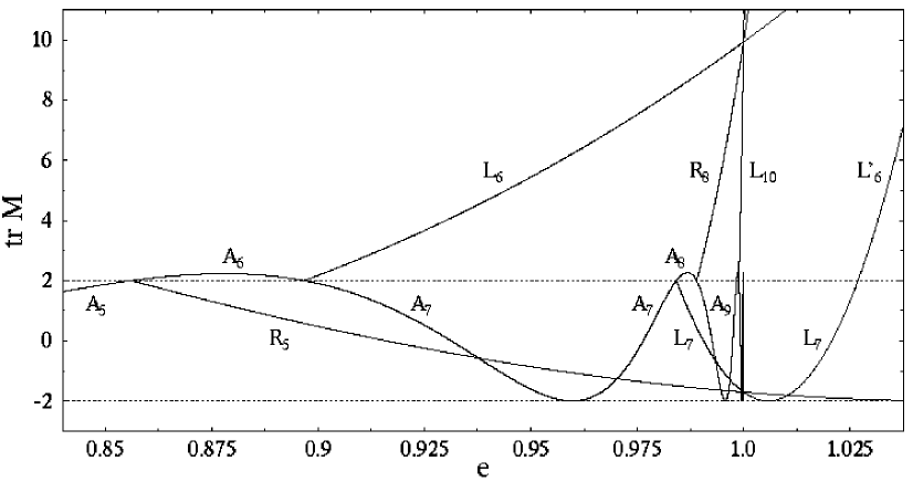
Figure 8: Stability discriminant of the shortest orbits in the H4 potential, plotted versus scaled energy $e$ (cf. Table 2 for the bifurcation energies). L₇ bifurcates at $e\sim 1.027$ and becomes L${}^{\prime}_{6}$.

The non-trivial period-doubling bifurcations in this potential are of island-chain type, and the orbits born thereby are given by Lamé functions of period 8K. We will not investigate them here, but refer to the analogous situation in the quartic oscillator potential discussed in Sec. 6.

In Fig. 8 we show the stability discriminant ${\rm tr\,M}$ versus energy $e$ for the orbit A and the orbits born at its lowest isochronous bifurcations. Different from the HH potential, here the functions ${\rm tr\,M}(e)$ of the bifurcated orbits are, to a good approximation, quadratic in $e$. This can be derived analytically [27]. It is also striking that, different from Fig. 2, ${\rm tr\,M}$ of all the orbits shown is always larger than or equal to $-2$. This behaviour, together with the systematics seen in Table 2, can be explained by the following arguments.

Bearing in mind that the stability matrix of the second iterate O² of a periodic orbit O is just M${}_{\rm O}^{2}$, where M_O is that of the primitive orbit, one easily finds that its discriminant is

$${\rm tr\,M}_{{\rm O}^{2}}={\rm tr\,M}^{2}_{\rm O}=({\rm tr\,M}_{\rm O})^{2}-2\,,$$ (43)

which can never be less than $-2$. Hence, we can mathematically understand ${\rm tr\,M}$ of the orbit A in Fig. 8 to be that of a second iterate. Its primitive is half of the orbit A, having the same period as that of the function ${\rm sn}^{2}$ in the Lamé equation for its stability, and having a discriminant ${\rm tr\,M}$ which oscillates around zero, exceeding the values $+2$ and $-2$ on both sides symmetrically, like ${\rm tr}\,{\rm M}_{\rm A}$ in the HH potential (Fig. 2). Their second iterates, which correspond to the full bifurcated orbits, therefore have a discriminant ${\rm tr\,M}$ which is quadratic in $e$. These features, together with the systematics in Table 2, are all a consequence of the C_4v symmetry of the H4 potential, including the reflection symmetry at the $x$ axis that divides the A orbit (and all the bifurcated orbits discussed here) into to equal halves. The quadratic behaviour of ${\rm tr\,M}$ of the bifurcated orbits is also consistent with the fact that their next period-doubling bifurcations (where ${\rm tr\,M}=-2$) are symmetry breaking (see Ref. [26] for details).

Like in the HH case, the values of ${\rm tr\,M}$ of the bifurcated orbits intersect in two points at $e=1$, one with ${\rm tr\,M}(e=1)=-1.711$ for the orbits born stable, and one with ${\rm tr\,M}(e=1)=+9.991$ for the orbits born unstable.

We thus obtain the result that Lamé functions with both periods 2K and 4K describe the orbits born at isochronous bifurcations of the A orbit. Two examples are shown in Figs. 9 and 10, where the $x$ motion of the orbits L₁₄ and R₁₆ is given by the functions Ec${}_{n}^{6}(z)$ and Es${}_{n}^{7}(z)$, respectively.

Figure 9: Same as Fig. 4 for the orbit L₁₄ in the H4 potential (cf. Table 2). Note that $x(t)$ has half the period of $y(t)$.

Whereas the latter shares its period with orbit A, the former has half its period. Like before, these orbits are evaluated at the critical energy $e=1$. The normalization of the Lamé functions has been chosen as for the HH potential, using the frozen-$y$-motion approximation and energy conservation, leading here to

$$x_{\sigma}(t_{0})=\sqrt{(e-e_{\sigma})/2(1+3y_{1})}\,\qquad{\dot{x}}_{\sigma}(t_{0})=\sqrt{(e-e_{\sigma})/2}\,.$$ (44)

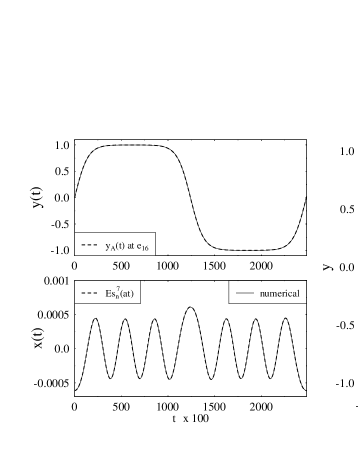
Figure 10: Same as Fig. 4 for the orbit R₁₆ in the H4 potential (cf. Table 2).

6 The homogeneous quartic oscillator

We now turn to the quartic oscillator (Q4) potential

$$V_{Q4}(x,y)=\frac{1}{4}\left(x^{4}+y^{4}\right)+\frac{\epsilon}{2}\,x^{2}y^{2}$$ (45)

which has been the object of several classical and semiclassical studies [31]. Since it is homogeneous in the coordinates, the Hamiltonian can be rescaled together with coordinates and time such that its classical mechanics is independent of energy. Consequently, the system parameter is here not the energy but the parameter $\epsilon$. The potential (45) has the same symmetry as the H4 potential (37) and, correspondingly, possesses periodic straight-line orbits along both axes. The motion of the A orbit along the $y$ axis is given by

$$y_{A}(t)=y_{0}\,{\rm cn}(y_{0}t,k)\,,\qquad y_{0}=(4E)^{1/4},\qquad k^{2}=1/2$$ (46)

with the period $T_{A}=4\,\hbox{\bf K}/y_{0}$. Its turning points are $\pm y_{0}$. Note that this solution does not depend on the value of $\epsilon$. The stability of the orbit A, however, does depend on $\epsilon$. The linearized equation of motion for the transverse $x$ motion yields, after transformation to the coordinate $z=y_{0}t$, the Hill equation

$$x^{\prime\prime}(z)+\epsilon\,[1-{\rm sn}^{2}(z,k)]\,x(z)=0\,.$$ (47)

This is a special case of the Lamé equation with

$$h=\epsilon=\frac{1}{2}\,n\,(n+1)\,,$$ (48)

where we have used $k^{2}=1/2$. The nice feature is that we here know analytically the eigenvalues $h=h_{n}$ of the Lamé equation, namely those given in Eq. (48). This agrees with the analytical result for the stability discriminant of the A orbit (46), which has been derived long ago by Yoshida [32]:

$${\rm tr}\,{\rm M}_{\rm A}=4\,\cos\left[\frac{\pi}{2}\sqrt{1+8\epsilon}\right]+2\,.$$ (49)

It is easy to see that the bifurcation condition ${\rm tr}\,{\rm M}_{\rm A}=+2$ leads exactly to the values (48) of the parameter $\epsilon$.

The periodic solutions of the Lamé equation (47) at the bifurcation values of $h=\epsilon$ are the Lamé polynomials discussed already in Sec. 3. Their explicit forms for $n=0,\,1,\,\dots,$ 15 are given in Table 3, using the short notation ${\rm cn}={\rm cn}(z,k)$, etc., and a normalization such that their leading coefficient is unity. We also give in Table 3 the names of the new-born orbits, using the same nomenclature as for the H4 potential in the previous section. Their shapes are shown in Fig. 11. They have exactly the same topologies as the orbits of the H4 potential and are again described by Lamé functions of pairwise alternating periods $2\hbox{\bf K}$ and $4\hbox{\bf K}$, as seen also in Table 3. Each of these orbits has a discrete degeneracy of 2, which is due to the time reversal symmetry for the rotations and to the reflection symmetries about the coordinate axes for the librations.

A special comment is due concerning the cases $n=1$ and $n=2$ which correspond to $\epsilon=1$ and 3, respectively. For these values of the parameter $\epsilon$, the Q4 potential is integrable [31, 32] and no bifurcations occur for the shortest orbits. Nevertheless, the Lamé equation (47) possesses mathematically the solutions Ec${}_{1}^{1}$ and Es${}_{2}^{1}$, respectively. The orbits B₃ and C₄ given in Table 3 and Fig. 11 have topologically the shapes given by these Lamé polynomials, but it should be emphasized that they are not generated through bifurcations but are generic orbits existing at all values of $\epsilon$. Under the symmetry operation $\epsilon\longrightarrow(3-\epsilon)/(1+\epsilon)$, which corresponds to a rotation about 45 degrees and simultaneous stretching of the potential [31], the orbits of type A are mapped onto the

$n$	$\epsilon_{n}$	Oσ	Lamé polynomial for $x(t)$	$P$
0	0	L3	Ec${}_{0}^{0}\;$ =  1	2K
1	1	[B3]	[Ec${}_{1}^{1}\;$ =  cn]	4K
2	3	[C4]	[Es${}_{2}^{1}\;$ =  dn sn]	4K
3	6	R5	Es${}_{3}^{2}\;$ =  cn dn sn	2K
4	10	L6	Ec${}_{4}^{2}\;$ =  $1-\frac{5}{3}\,{\rm cn}^{4}$	2K
5	15	L7	Ec${}_{5}^{3}\;$ =  cn ($1-\frac{7}{5}\,{\rm cn}^{4}$)	4K
6	21	R8	Es${}_{6}^{3}\;$ =  dn sn ($1-3\,{\rm cn}^{4}$)	4K
7	28	R9	Es${}_{7}^{4}\;$ =  cn dn sn ($1-\frac{11}{5}\,{\rm cn}^{4}$)	2K
8	36	L10	Ec${}_{8}^{4}\;$ =  $1-6\,{\rm cn}^{4}+\frac{39}{7}\,{\rm cn}^{8}$	2K
9	45	L11	Ec${}_{9}^{5}\;$ =  cn ($1-\frac{22}{5}\,{\rm cn}^{4}+\frac{11}{3}\,{\rm cn}^{8}$)	4K
10	55	R12	Es${}_{10}^{5}$ =  dn sn ($1-\frac{26}{3}\,{\rm cn}^{4}+\frac{221}{21}\,{\rm cn}^{8}$)	4K
11	66	R13	Es${}_{11}^{6}$ =  cn dn sn ($1-6\,{\rm cn}^{4}+\frac{19}{3}\,{\rm cn}^{8}$)	2K
12	78	L14	Ec${}_{12}^{6}$ = ($1-13\,{\rm cn}^{4}+\frac{221}{7}\,{\rm cn}^{8}-\frac{221}{11}\,{\rm cn}^{12}$)	2K
13	91	L15	Ec${}_{13}^{7}$ =  cn ($1-9\,{\rm cn}^{4}+19\,{\rm cn}^{8}-\frac{437}{39}\,{\rm cn}^{12}$)	4K
14	105	R16	Es${}_{14}^{7}$ =  dn sn ($1-17\,{\rm cn}^{4}+51\,{\rm cn}^{8}-\frac{425}{11}\,{\rm cn}^{12}$)	4K
15	120	R17	Es${}_{15}^{8}$ =  cn dn sn ($1-\frac{57}{5}\,{\rm cn}^{4}+\frac{437}{15}\,{\rm cn}^{8}-\frac{1311}{65}\,{\rm cn}^{12}$)	2K

Table 3:  Numbers $n$ and parameter values $\epsilon_{n}$ for the isochronous bifurcations of the A orbit in the homogeneous quartic oscillator (Q4) potential; names O_σ of bifurcated orbits; Lamé polynomials for their $x$ motion, and their periods $P$. The Jacobi elliptic functions sn, cn, and dn are given in short notation as ${\rm sn}={\rm sn}(z,k)$, etc., with $z=y_{0}t$, where $y_{0}$ and the modulus $k$ are given in (46). (See text for a special comment on orbits B₃ and C₄.)

orbits of type B and vice versa, and the orbits of type C are mapped onto themselves. This is seen easily in the Lamé polynomial describing the B orbit, Ec${}_{1}^{1}(z)$ = cn$(z,k)$, which is proportional to the function (46) describing the A orbit.

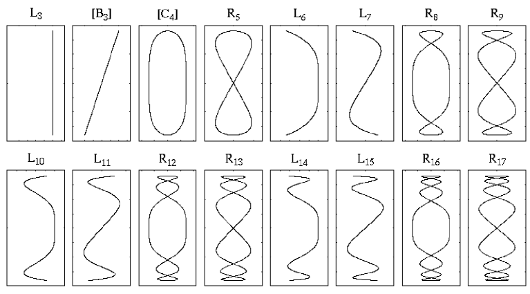
Figure 11: Shapes of orbits born at the isochronous bifurcations of orbit A in the Q4 potential. Vertical direction: $y_{A}(t)$ given by (46); horizontal direction: $x(t)$ given by the Lamé polynomials listed in Table 3 (with scaled normalizations to fit the shapes into the frames).

The scaling properties of these orbits and their evolution away from the bifurcation values $\epsilon_{\sigma}$ are more difficult to analyze than in the HH and H4 potentials and will be discussed elsewhere [33].

We now discuss period-doubling bifurcations of the A orbit in the Q4 potential. There is a series of trivial period doublings which just involve the second iterates of the orbit A and the orbits born at its isochronous bifurcations and listed in Table 3. The non-trivial period doublings occur when ${\rm tr}\,{\rm M}_{\rm A}=-2$, which leads with (49) to the critical values

$$\epsilon=2\,p\,(p+1)+3/8\,,\qquad p=0,1,2,\dots$$ (50)

This is exactly one of the conditions [9] for the existence of period-8K solutions of (47), namely that obtained by inserting $n=(4p+1)/2$ into Eq. (48). The solutions are the algebraic Lamé functions, given (up to $p=3$) in Table 4 below. These bifurcations are of the island-chain type (see, e.g., Ref. [28]): the quantity tr M of the second iterate of orbit A – let us call it orbit A² – touches the value $+2$, but the orbit A² remains stable on either side. At the bifurcation, two doubly-degenerate orbits are born, one stable and one unstable. The situation is illustrated in Fig. 12 around the bifurcation at $\epsilon=4+3/8$ ($p=1$). The unstable new orbit is here called F₁₀, and the stable new orbit is called P₉. There shapes, together with those born at the other period doublings listed in Table 4, are shown in Fig. 13 below. Their degenerate symmetry partners are called F${}^{\prime}_{\sigma}$ for the librating orbits (obtained by reflecting the F_σ orbits at the $x$ axis) and P${}^{\prime}_{\sigma}$ for the rotating orbits (obtained by time reversal of the P_σ orbits).

According to the theory of Ince [9], the algebraic Lamé functions of period 8K are one exceptional case where two independent periodic solutions can coexist for the same critical value of $h$. These are the functions Ec${}_{2p+1/2}^{\,p+1/2}$ and Es${}_{2p+1/2}^{\,p+1/2}$ defined in Eqs. (23,24). As we see from Table 4, they correspond to the unstable orbits of type F_σ and F${}^{\prime}_{\sigma}$. In contrast to the degenerate pairs of bifurcated orbits in the HH and H4 potentials, which are represented by one and the same periodic Lamé function, the pairs F_σ and F${}^{\prime}_{\sigma}$ are here given by two linearly independent functions. With this, however, the number of independent solutions of the second-order differential equation (47) is exhausted. Therefore the other pair of stable orbits of type P_σ and P${}^{\prime}_{\sigma}$ born at the period doublings cannot be given by any new independent solutions. Indeed, we see from Table 4 that the orbits P_σ and P${}^{\prime}_{\sigma}$ are

Figure 12: Stability discriminant ${\rm tr\,M}$ of period-2 orbits in the Q4 potential around a period-doubling bifurcation of island-chain type at $\epsilon=4.375$. A² is the second iterate of the primitive orbit A₅ (shown by a dashed line); its Maslov index increases from 9 to 11 at the bifurcation. F₁₀ and P₉ are the genuine period-2 orbits bifurcating from it; each has a discrete degeneracy of two (see text and Table 4); P₉ bifurcates at $\epsilon\simeq 5.3$ and becomes P₈.

$n\!$	$\epsilon_{n}\!$	O${}_{\sigma}\!$	algebraic Lamé function for $x(t)$
$\frac{1}{2}\!$	$\frac{3}{8}\!$	F${}_{6}\!$	Ec${}_{1/2}^{1/2}$ = $\!\sqrt{{\rm dn}+{\rm cn}}$
		F${}^{\prime}_{6}\!$	Es${}_{1/2}^{1/2}$ = $\!\sqrt{{\rm dn}-{\rm cn}}$
		P${}_{7}\!$	$\sqrt{{\rm dn}+{\rm cn}}\,+\sqrt{{\rm dn}-{\rm cn}}$
		P${}^{\prime}_{7}\!$	$\sqrt{{\rm dn}+{\rm cn}}\,-\sqrt{{\rm dn}-{\rm cn}}$
$\frac{5}{2}\!$	$4\frac{3}{8}\!$	F${}_{10}\!$	Ec${}_{5/2}^{3/2}$ = $\!\sqrt{{\rm dn}+{\rm cn}}\,(1-\frac{4}{7}\,{\rm sn}^{2}-\frac{8}{7}\,{\rm dn}\,{\rm cn})$
		F${}^{\prime}_{10}\!$	Es${}_{5/2}^{3/2}$ = $\!\sqrt{{\rm dn}-{\rm cn}}\,(1-\frac{4}{7}\,{\rm sn}^{2}+\frac{8}{7}\,{\rm dn}\,{\rm cn})$
		P${}_{9}\!$	Ec${}_{5/2}^{3/2}\;+\;$Es${}_{5/2}^{3/2}$
		P${}^{\prime}_{9}\!$	Ec${}_{5/2}^{3/2}\;-\;$Es${}_{5/2}^{3/2}$
$\frac{9}{2}\!$	$12\frac{3}{8}\!$	F${}_{14}\!$	Ec${}_{9/2}^{5/2}$ = $\!\sqrt{{\rm dn}+{\rm cn}}\,(1-\frac{36}{13}\,{\rm sn}^{2}+\frac{16}{13}\,{\rm sn}^{4}-\frac{8}{13}\,{\rm dn}\,{\rm cn})$
		F${}^{\prime}_{14}\!$	Es${}_{9/2}^{5/2}$ = $\!\sqrt{{\rm dn}-{\rm cn}}\,(1-\frac{36}{13}\,{\rm sn}^{2}+\frac{16}{13}\,{\rm sn}^{4}+\frac{8}{13}\,{\rm dn}\,{\rm cn})$
		P${}_{13}\!$	Ec${}_{9/2}^{5/2}\;+\;$Es${}_{9/2}^{5/2}$
		P${}^{\prime}_{13}\!$	Ec${}_{9/2}^{5/2}\;-\;$Es${}_{9/2}^{5/2}$
$\frac{13}{2}\!$	$24\frac{3}{8}\!$	F${}_{18}\!$	Ec${}_{13/2}^{7/2}$ =$\,\sqrt{{\rm dn}+{\rm cn}}\,[1-\frac{1304}{347}\,{\rm sn}^{2}+\frac{1200}{347}\,{\rm sn}^{4}-\frac{320}{347}\,{\rm sn}^{6}+\frac{272}{347}\,{\rm dn}\,{\rm cn}\,(1-\frac{40}{17}\,{\rm cn}^{4})]\!$
		F${}^{\prime}_{18}\!$	Es${}_{13/2}^{7/2}$ =$\,\sqrt{{\rm dn}-{\rm cn}}\,[1-\frac{1304}{347}\,{\rm sn}^{2}+\frac{1200}{347}\,{\rm sn}^{4}-\frac{320}{347}\,{\rm sn}^{6}-\frac{272}{347}\,{\rm dn}\,{\rm cn}\,(1-\frac{40}{17}\,{\rm cn}^{4})]\!$
		P${}_{17}\!$	Ec${}_{13/2}^{7/2}\;+\;$Es${}_{13/2}^{7/2}$
		P${}^{\prime}_{17}\!$	Ec${}_{13/2}^{7/2}\;-\;$Es${}_{13/2}^{7/2}$

Table 4:  Numbers $n$ and parameter values $\epsilon_{n}$ of the four lowest non-trivial period-doubling bifurcations of the A orbit in the homogeneous quartic oscillator. Given are also the names O_σ of the four topologically different orbits born simultaneously at these bifurcations, and the (linear combinations of) algebraic Lamé functions with period 8K that describe their $x$ motion. (The same short notation for the Jacobi elliptic functions sn, dn and cn is used as in Table 3.)

given by the two independent linear combinations Ec${}_{2p+1/2}^{p+1/2}\,\pm$ Es${}_{2p+1/2}^{p+1/2}$ which were constructed by Erdélyi [16] to have the same symmetry properties as those of the 2K and 4K periodic Lamé functions, as discussed in Sec. 3.

We thus have found the interesting result – which was new to us – that the stable and unstable pairs of orbits born at a period-doubling bifurcation of island-chain type are mutually linear combinations of each other. It follows from our above arguments that this result must hold for all Hamiltonians with the double reflection symmetry C_2v.

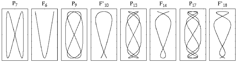
Figure 13: Same as Fig. 11, but for orbits born at period-doubling bifurcations of orbit A in the Q4 potential. The motion $x(t)$ is given by the algebraic Lamé functions listed in Table 4.

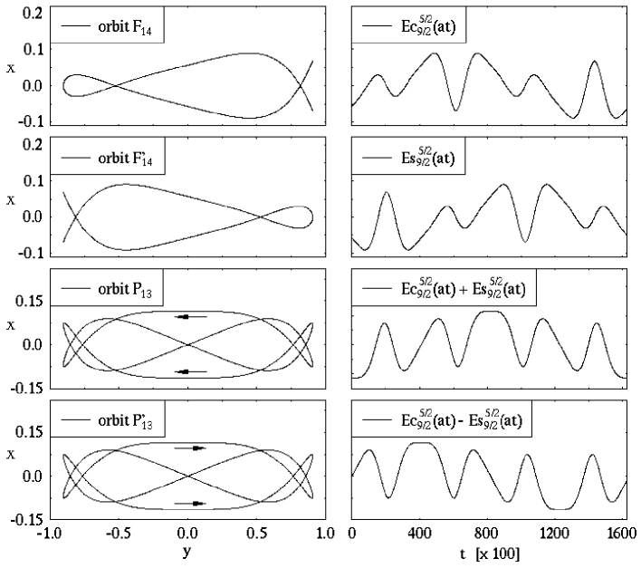
Figure 14: The four orbits born at the period-doubling bifurcation at $\epsilon=12.375$. Left: their shapes in the $(x,y)$ plane; right: algebraic Lamé functions describing their motion $x(t)$.

In Fig. 14 we illustrate the situation for the four orbits born at the bifurcation at $\epsilon=12+3/8$ ($p=2$). In the left panels, their shapes $x(y)$ are shown; in the right panels we plot the algebraic Lamé functions (and their linear combinations) which describe the motion $x(t)$ of the respective orbits. Looking merely at the shapes of these orbits, the pairwise linear dependence of their $x$ motion is not obvious at all.

7 Summary and conclusions

We have investigated cascades of isochronous pitchfork bifurcations of straight-line librational orbits in two-dimensional potentials. The linearized equation of the $x$ motion transverse to these orbits, determining their stability, can be written in the form of the Lamé equation. Its eigenvalues correspond to the bifurcation values of the system parameter, given also by the condition tr M$=+2$ for the stability discriminant of the straigh-line orbit, and its eigenfunctions describe the $x$ motion of the new orbits born at the bifurcations. These eigenfunctions are the periodic Lamé functions of period $2\hbox{\bf K}$ or $4\hbox{\bf K}$, where K is the complete elliptic integral determining the period of the parent orbit at the corresponding bifurcation. In potentials with C_2v symmetry, the solutions occur alternatingly as Lamé functions of period 2K and 4K, respectively. When this symmetry is absent, the $4\hbox{\bf K}$ periodic solutions describe the orbits born at period-doubling pitchfork bifurcations.

We have shown numerically that the periodic Lamé functions describe very accurately the shapes of the bifurcated orbits obtained from a numerical integration of the equations of motion, as long as the amplitude of their $x$ motion remains small, i.e., as long as one is not too far from the bifurcation point. Exploiting the energy conservation in the Hénon-Heiles type potentials HH and H4 and the known symmetries of the Lamé functions, we can predict the propagation of the new orbits up to the critical saddle-point energy where they have all become unstable and the system is highly chaotic. We thus have found an analytical description of an infinite series of unstable periodic orbits in chaotic systems.

In the homogeneous quartic oscillator (Q4) potential, the series expansions of the periodic Lamé functions terminate and they become finite polynomials. In this potential we have also analyzed solutions of period $8\hbox{\bf K}$ which occur at period-doubling bifurcations of the straight-line orbits of island-chain type. The two pairs of orbits born thereby are represented by two independent sets of orthogonal periodic solutions of the Lamé equation, which here are identified with the so-called algebraic Lamé functions that can again be given in a closed form.

Similar cascades of pitchfork bifurcations have also been discussed in connection with the diamagnetic Kepler problem represented by hydrogen atoms in strong magnetic fields [25, 34, 35]. Expressing the Hamiltonian in (scaled) semiparabolic coordinates $(u,v)$, the effective potential for orbits with angular momentum $L_{z}=0$ (where the $z$ axis is the direction of the external magnetic field) becomes similar to the H4 and Q4 potentials discussed here (although it contains only quadratic and sixth-order terms in the coordinates). Since physically the $(u,v)$ coordinates are positive definite, the periodic orbits in the diamagnetic Kepler problem correspond to the half-orbits of the H4 and the Q4 potentials. There exist straight-line librating orbits, corresponding to oscillations of the electron along the symmetry axis, which bifurcate infinitely many times as the energy of the electron approaches the ionization threshold. The stability of these linear orbits is given by the Mathieu equation, which is analogous to the Lamé equation (6) but with the function sn${}^{2}(z,k)$ replaced by $\cos(2z)$. Its periodic solutions are the periodic Mathieu functions se_m and ce_m which have properties completely analogous to those of the periodic Lamé functions, and were actually studied in detail by Ince [36] prior to his investigations of the Lamé functions. The topology of the Mathieu functions and of the bifurcated orbits described by them is exactly the same as for the Q4 and H4 potentials described here. In particular, the so-called “balloon” orbits B_n and “snake” orbits S_n with $n=1,$ 2, $\dots$ [25] correspond exactly to the alternating sequence of halves of the orbits R₅, R₉, $\dots$ and L₇, L₁₁, $\dots$ shown in Fig. 11. (The other orbits, born unstable at the bifurcations, were not considered in [25] since they do not pass through the centre.) We believe that our analysis, applied in terms of the Mathieu functions, may be useful for further investigations of the bifurcations occurring in the diamagnetic Kepler problem.

The knowledge of the analytical properties of the bifurcated orbits will be useful in the application of the periodic orbit theory to the potentials studied here. First steps in this direction have been quite successful [29, 30, 37], but the orbits bifurcated from the A orbit were not considered. Their incorporation into the semiclassical trace formula is the object of further work in progress. We expect the bifurcated orbits, in particular, to play an important role in the semiclassical analysis of resonances above the barriers in Hénon-Heiles type or similar potentials.

Acknowledgments

We are grateful to S Fedotkin and A Magner for very stimulating discussions and critical comments. Valuable comments by M Sieber and H Then are highly appreciated. We also acknowledge financial support by the Deutsche Forschungsgemeinschaft.

References

- [1]
-
[2]
Feigenbaum M J 1978 J. Stat. Phys. 19 25
see also Feigenbaum M J 1983 Physica 7 D 16 - [3] Bountis T C 1981 Physica 3 D 577
- [4] Greene J M, McKay R S, Vivaldi F and Feigenbaum M J 1981 Physica 3 D 577
- [5] Brack M 2001 Festschrift in honor of the 75th birthday of Martin Gutzwiller ed A Inomata et al Foundations of Physics 31 209 [LANL preprint nlin.CD/0006034]
-
[6]
Lamé G 1839 Journal de Mathématiques Pures et
Appliquées (Liouville) 4 126
Lamé G 1839 ibid. 4 351 - [7] see, e.g., Strutt M J O 1932 Ergebnisse der Mathematik und ihrer Grenzgebiete Vol. 1 no. 3 (Springer-Verlag, Berlin)
- [8] Ince E L 1940 Proc. Royal Soc. Edinburgh 60 47
- [9] Ince E L 1940 Proc. Royal Soc. Edinburgh 60 83
- [10] Hénon M and Heiles C 1964 Astr. J. 69 73
- [11] Hill G W 1886 Acta Math. 8 1
- [12] Magnus W and Winkler S 1966 Hill’s Equation (Interscience Publ., New York)
-
[13]
Erdélyi A et al 1955 Higher Transcendental
Functions Vol III (McGraw-Hill, New York) ch 15.
Beware of the misprint in equation (13) and elsewhere in chapter 15.5.1 of this reference; the correct definition of the variable is that given in Eq. (8) of our present paper - [14] Gradshteyn I S and Ryzhik I M 1994 Table of Integrals, Series, and Products (Academic Press, New York, 5th edition) ch 8.1
- [15] Erdélyi A 1941 Phil. Mag. (7) 31 123
- [16] Erdélyi A 1941 Phil. Mag. (7) 32 348
- [17] Tanaka K and Brack M, to be published
- [18] Churchill R C, Pecelli G and Rod D L 1979 Stochastic Behavior in Classical and Quantum Hamiltonian Systems ed G Casati and J Ford (Springer-Verlag, New York) p 76
- [19] Davies K T R, Huston T E and Baranger M 1992 Chaos 2 215
- [20] Vieira W M and Ozorio de Almeida A M 1996 Physica 90 D 9
- [21] Gutzwiller M C 1971 J. Math. Phys. 12 343
- [22] Gutzwiller M C 1990 Chaos in classical and quantum mechanics (Springer, New York)
- [23] Brack M and Bhaduri R K 1997 Semiclassical Physics, Frontiers in Physics Vol. 96 (Addison-Wesley, Reading, USA)
- [24] de Aguiar M A M, Malta C P, Baranger M, and Davies K T R 1987 Ann. Phys. (NY) 180 167
- [25] Mao J-M and Delos J B 1992 Phys. Rev. A 45 1746
-
[26]
Then H L 1999 Diploma thesis (Universität Ulm)
Then H L and Sieber M, to be published - [27] Fedotkin S N, Magner A G, Mehta M and Brack M, to be published
-
[28]
Sieber M 1996 J. Phys. A 29 4715
Schomerus H and Sieber M 1997 J. Phys. A 30 4537
Sieber M and Schomerus H 1998 J. Phys. A 31 165 - [29] Brack M, Creagh S C and Law J 1998 Phys. Rev. A 57 788
- [30] Brack M, Meier P and Tanaka K 1999 J. Phys. A 32 331
-
[31]
Eckardt B 1988 Phys. Rep. 163 205
Bohigas O, Tomsovic S and Ullmo U 1993 Phys. Rep. 233 45
Eriksson A B and Dahlqvist P 1993 Phys. Rev. E 47 1002
Lakhshminarayan A, Santhanam M S, and Sheorey V B 1996 Phys. Rev. Lett. 76 396 - [32] Yoshida H 1984 Celest. Mech. 32 73. Strictly speaking, Yoshida derived tr M for the half-orbit to be tr M, from which Eq. (49) follows using Eq. (43)
- [33] Mehta M and Brack M, work in progress
-
[34]
Main J, Wiebusch G, Holle A and Welge K H 1986 Phys. Rev. Lett. 57 2789
Main J, Wiebusch G, Holle A and Welge K H 1987 Z. Phys. D 6 295 -
[35]
Wintgen D and Friedrich F 1987 Phys. Rev. A 36 131
Friedrich F and Wintgen D 1989 Phys. Rep. 183 39
Hasegawa H, Robnik M and Wunner G 1989 Prog. Th. Phys. Suppl. 98 198 - [36] Ince E L 1932 Proc. Royal Soc. Edinburgh 52 355
-
[37]
Brack M, Bhaduri R K, Law J and Murthy M V N 1993
Phys. Rev. Lett. 70 568
Brack M, Bhaduri R K, Law J, Maier Ch and Murthy M V N 1995 Chaos 5 317,707(E)