Slow energy relaxation and localization in 1D lattices

Abstract

We investigate the energy relaxation process produced by thermal baths at zero temperature acting on the boundary atoms of chains of classical anharmonic oscillators. Time–dependent perturbation theory allows us to obtain an explicit solution of the harmonic problem: even in such a simple system nontrivial features emerge from the interplay of the different decay rates of Fourier modes. In particular, a crossover from an exponential to an inverse–square–root law occurs on a time scale proportional to the system size $N$. A further crossover back to an exponential law is observed only at much longer times (of the order $N^{3}$). In the nonlinear chain, the relaxation process is initially equivalent to the harmonic case over a wide time span, as illustrated by simulations of the $\beta$ Fermi–Pasta–Ulam model. The distinctive feature is that the second crossover is not observed due to the spontaneous appearance of breathers, i.e. space–localized time–periodic solutions, that keep a finite residual energy in the lattice. We discuss the mechanism yielding such solutions and also explain why it crucially depends on the boundary conditions.

submitted to: J. Phys. A, Math. Gen.

PACS: 63.20.Ry, 63.20.Pw

Corresponding author: Francesco Piazza, piazza@phy.hw.ac.uk

1 Introduction

The concept of discrete breathers (DB) has been brought to the foreground by recent studies on the dynamical properties of anharmonic lattices [1]. DB are space–localized time–periodic solutions, with frequencies lying out of the linear spectrum and they have been proved to exist in a wide class of models [2]. Although a fairly large amount of rigorous and numerical work has been devoted to the identification of the conditions for their existence and stability, much less is known about their possible relevance for the thermodynamic properties of lattices, both at and out of equilibrium. The latter case includes transient dynamics, e.g. relaxation to equipartition  [3], and stationary heat transport [4].

An important example of the role played by DB in determining relaxation properties has been provided by Tsironis and Aubry [5]. They have shown that a characteristic slow relaxation behaviour of the energy emerges when a nonlinear chain prepared in a typical thermalized state, corresponding to a given finite temperature, is put in contact with a cold bath. This physical setup can be simulated by a damping term acting on a number of boundary particles. The system eventually reaches a state where a residual finite amount of the initial energy is kept under the form of DB. In a subsequent numerical work [6] it has been further argued that the energy relaxation should obey a stretched–exponential law in time.

Although such a behaviour is considered on its own a signature of complex dynamics, its origin remains not completely understood, even in the more widely studied problem of glassy relaxation [7]. Loosely speaking, it is usually attributed to a multiple–local–minima structure in the energy landscape of the system. This would originate metastable states capable of trapping the configuration of the system during the relaxation, thus giving rise to a very slow decay. In some cases it is also assumed that this behaviour is the result of the competition between two (or among many) pure exponential processes [7]. Otherwise, it has been proposed to stem from a complex activation mechanism, whereby different degrees of freedom “defreeze” at later and later stages. This constitutes a hierarchical scheme, with faster degrees of freedom successively constraining the slower ones [8].

Beyond the possible relevance of these different scenarios, it is important to have a definite quantitative description of the relaxation phenomenon in connection with energy localization. With this paper we aim to settle these issues on a firm basis, showing also that the picture is more subtle than one might naively expect. As a first step, we consider the simple but very instructive case of the harmonic chain, with damping acting on its edge particles. This exercise shows indeed how a slower–than–exponential relaxation arises as a global effect from the existence of different time scales of the Fourier modes. As a matter of fact, only a linear system with damping on each particle would display simple exponential relaxation. More specifically, a perturbative calculation reveals that the energy decay law exhibits a first crossover from an exponential to an inverse–square–root law. The corresponding crossover time $\tau_{0}$ is inversely proportional to the product of the damping constant times the fraction of damped particles.

These results turn out to be extremely useful to be compared with the nonlinear case. Remarkably, the only difference concerns the long–time behaviour of the decay process. Indeed, in the linear system we observe a second crossover back to an exponential law, while in the nonlinear one the energy converges to a finite asymptotic value, due to spontaneous localization of the energy in the form of DB. However, we find that finite–size effects both in space and time may prevent energy localization, making the interpretation of the energy decay process more subtle and interesting.

The paper is organized as follows. In section 2 we describe the general features of the relaxation dynamics and illustrate the typical layout of numerical simulations. The results obtained for the linear system are discussed in section 3; section 4 is devoted to the study of the relaxation process in the $\beta$ Fermi–Pasta–Ulam (henceforth FPU) model (e.g. a quartic nonlinearity in the interparticle potential) and is known to allow for the existence of breather states. Finally, we summarize and draw our conclusions in section 5.

2 Generalities of the relaxation dynamics

We consider a homogeneous chain of $N$ atoms of mass $m$ and denote with $u_{p}$ the displacement of the $p$-th particle from its equilibrium position at time $t$ (for the sake of simplicity in what follows we omit the explicit dependence on time). The atoms are labelled by the integer space index $p=0,1,\dots N-1$. In the nearest–neighbour approximation of the interactions the equations of motion read

$$\ \ \ \ \ m\ddot{u}_{p}=V^{\prime}(u_{p+1}-u_{p})-V^{\prime}(u_{p}-u_{p-1})-m\sum_{p^{\scriptscriptstyle\prime}=0}^{N-1}\Gamma_{pp^{\scriptscriptstyle\prime}}\dot{u}_{p^{\scriptscriptstyle\prime}},$$ (1)

where $V(x)$ is the interparticle potential, for which we assume that $V^{\prime}(0)=0$, denoting with $V^{\prime}(x)$ the derivative of $V(x)$ with respect to $x$. The last term in eq. (1) represents the interaction of the atoms with a “zero temperature” heat bath in the form of a linear damping, characterized by the coupling matrix $\Gamma$. In what follows we consider the case in which dissipation acts only on the atoms located at the chain edges, so that $\Gamma$ has the form

$$\Gamma_{pp^{\scriptscriptstyle\prime}}=\gamma\delta_{p^{\scriptscriptstyle\prime},p}\left[\delta_{p^{\scriptscriptstyle\prime},0}+\delta_{p^{\scriptscriptstyle\prime},N-1}\right]\quad,$$ (2)

where $\gamma$ is the damping constant and $\delta_{p^{\scriptscriptstyle\prime},p}$ is the Kronecker delta. As we are dealing with systems in a finite volume we impose either free–end ($u_{-1}=u_{0}$, $u_{N-1}=u_{N}$) or fixed–end ($u_{-1}=u_{N}=0$) boundary conditions (BC).

The numerical investigations reported in this paper have been performed according to the following procedure. We integrate equations (1) starting from a microcanonical equilibrium condition corresponding to a given energy density $E(0)/N$. This condition is obtained by letting the hamiltonian system ($\gamma=0$) perform a short microcanonical transient, whose duration is typically ${\cal O}(10^{3})$ time units. The initial condition for such transient is assigned by drawing momenta from a Gaussian distribution corresponding to the desired energy, while all displacement variables $u_{p}$ are set to zero. During the hamiltonian transient the equations of motion are integrated by means of a 5–th order symplectic Runge–Kutta–Nyström algorithm [9], while a standard 4–th order Runge–Kutta algorithm is used for the dissipative dynamics.

It is useful to introduce the so–called symmetrized site energies

$$e_{p}\;=\;\frac{1}{2}m\dot{u}_{p}^{2}+\frac{1}{2}\left[V(u_{p+1}-u_{p})+V(u_{p}-u_{p-1})\right].$$

The istantaneous total energy of the system is then given by

$$E=\sum_{p=0}^{N-1}e_{p}.$$ (3)

Due to the presence of dissipation, the initial energy $E(0)$ decreases in time. Since we are interested in determining the decay law of the normalized quantity $E(t)/E(0)$, it is convenient to introduce the following indicator

$${\cal D}(t)=\log[-\log(E(t)/E(0))].$$ (4)

By plotting ${\cal D}$ versus time in a log–lin scale, a streched–exponential law of the form $E(t)/E(0)=\exp[-(t/\tau)^{\sigma}]$ becomes a straight line with slope $\beta$ that intercepts the $y$–axis at $-\beta\log(\tau)$. As we shall see later on, this representation is very useful for identifying pure exponential regimes ($\sigma=1$) and the crossover to slower decay laws.

Since we are also interested in the effects of DB formation on the relaxation process, we introduce a localization parameter ${\cal L}$, which provides a rough estimate of the degree of energy localization in the system. We define it as

$${\cal L}(t)=N\,\frac{\displaystyle\sum_{p}e_{p}^{2}(t)}{\displaystyle\left[\sum_{p}e_{p}(t)\right]^{2}}.$$ (5)

Accordingly, the fewer sites the energy is localized onto, the closer ${\cal L}$ is to $N$. On the other hand, the more evenly the energy is spread on all the particles, the closer ${\cal L}$ is to a constant of order 1. For instance, in the latter case ${\cal L}$ for the FPU potential lies within the interval [7/4, 19/9], the two extremes being the energy–independent values of the harmonic and pure quartic potentials, respectively [3].

In order to smooth out fluctuations, both ${\cal D}(t)$ and ${\cal L}(t)$ have been averaged over different realizations (typically 20) of the equilibrium initial conditions.

3 The harmonic chain

In this section we discuss the results obtained for the 1D harmonic lattice,

$$V(x)=\frac{1}{2}k_{2}x^{2},$$

with both free–end and fixed–end BC. In order to solve the problem, we can use ordinary time–dependent perturbation theory, provided the damping constant $\gamma$ is small enough. We note that, since the number of the damped particles is fixed, the perturbative approximation is expected to improve by increasing the system size $N$. In the following we shall adopt adimensional units such that $k_{2}=m=a=1$, where $a$ is the lattice spacing. As a consequence, time is measured in units of $1/\omega_{0}$, where $\omega_{0}=\sqrt{4k_{2}/m}$ is the maximum frequency of the linear spectrum.

Let $-\omega^{2}_{\alpha}$ and $\eta^{\alpha}$ ($\alpha=0,1,\dots N-1$) denote the eigenvalues and normalized eigenvectors, respectively, of the unperturbed hamiltonian problem, where

$$\omega_{\alpha}^{2}=4\,\sin^{2}\left(\frac{q_{\alpha}}{2}\right)\quad.$$

and the wave–number $q_{\alpha}$ is defined in the Appendix (see eqs. A.6 and A.7) .

In the spirit of time–dependent perturbation theory we look for solutions of the form

$$u_{p}(t)=\sum_{\alpha=0}^{N-1}c_{\alpha}(t)e^{-i\omega_{\alpha}t}\eta_{p}^{\alpha}.$$ (6)

where $\eta_{p}^{\alpha}$ is the $p$-th component of the eigenvector $\eta^{\alpha}$. By substituting expression (6) in the equations of motion, we can rewrite them in the form of a system of differential equations for the $c_{\alpha}$’s. We can then find approximate solutions by expressing the latter as power series in the adimensional perturbation parameter $\gamma/\omega_{0}$. The details of the calculation are reported in the Appendix. To first order in $\gamma/\omega_{0}$ we obtain

$$c_{\alpha}(t)=c_{\alpha}(0)\exp\left[-\frac{t}{\tau_{\alpha}}\right],$$ (7)

where

$$\frac{1}{\tau_{\alpha}}=\frac{1}{\tau_{0}}\,\cos^{2}\left(\frac{q_{\alpha}}{2}\right),$$ (8)

and

$$\frac{1}{\tau_{\alpha}}=\frac{1}{\tau_{0}}\,\sin^{2}(q_{\alpha})$$ (9)

for the free–end and the fixed–end system, respectively, where $\tau_{0}=N/2\gamma$. We also note that, as a result of the calculation, the damping term introduces a correction of the normal frequencies. However, it is straightforward to verify that such a correction is of second order in the perturbation parameter and, accordingly, it can be neglected.

As we see from equations (8) and (9), the spectra of the decay rates are substantially different for the free–end and fixed–end BC. In the former case, we see that the least damped modes are the short–wavelength ones ($\alpha\approx N$), the largest lifetime being $\tau_{\scriptscriptstyle N-1}\approx 2N^{3}/\pi^{2}\gamma$, while the most damped modes are the ones in the vicinity of $\alpha=0$, with $\tau_{0}$ being the shortest decay time. On the contrary, for the fixed–end chain the most damped modes are the ones around $\alpha\approx N/2$, while both the short–wavelength and long–wavelength modes are very little damped, being $\tau_{\scriptscriptstyle N-1}\approx N(N+1)^{2}/2\pi^{2}\gamma$.

Using the definition of the system energy (3) and the solution (7), we can explicitely evaluate the normalized system energy as

$$\frac{E(t)}{E(0)}=\frac{\displaystyle\sum_{\alpha}c^{2}_{\alpha}(0)\omega_{\alpha}^{2}\,e^{-2t/\tau_{\alpha}}}{\displaystyle\sum_{\alpha}c^{2}_{\alpha}(0)\omega_{\alpha}^{2}}.$$ (10)

As we are interested in the typical behaviour of the system when it evolves from equilibrium initial conditions, we replace $c^{2}_{\alpha}(0)\omega_{\alpha}^{2}$ with its average value $2E(0)/N$. Thus, recalling equations (8) and (9) and approximating for large $N$ the sum over $\alpha$ with an integral ($\tau_{\alpha}\to\tau(q)$), we have

$$\frac{E(t)}{E(0)}=\frac{1}{\pi}\int_{0}^{\pi}e^{-\frac{\displaystyle 2t}{\displaystyle\tau(q)}}\,dq=e^{-\frac{\displaystyle t}{\displaystyle\tau_{\scriptscriptstyle 0}}}I_{\scriptscriptstyle 0}\left(\frac{\displaystyle t}{\displaystyle\tau_{\scriptscriptstyle 0}}\right)$$ (11)

where $I_{\scriptscriptstyle 0}$ is the modified zero–order Bessel function.

Surprisingly enough, although the mode relaxation rates are different in the free–end and fixed–end systems, the global result for the energy decay turns out to be the same. The asymptotic behaviour of the function (11) is given by

$$\frac{E(t)}{E(0)}=\left\{\begin{array}[]{ll}e^{\displaystyle-t/\tau_{\scriptscriptstyle 0}}&\ {\rm for}\ t\ll\tau_{\scriptscriptstyle 0},\\ \frac{\displaystyle 1}{\displaystyle\sqrt{2\pi(t/\tau_{\scriptscriptstyle 0})}}&\ {\rm for}\ t\gg\tau_{\scriptscriptstyle 0}.\end{array}\right.$$ (12)

Hence, $\tau_{\scriptscriptstyle 0}$ sets the time scale of a crossover from the initial exponential decay, led by the longest lifetime, to a power–law decay.

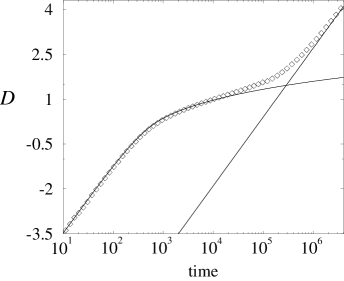
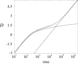
Figure 1: Symbols represent ${\cal D}$ versus time for a harmonic chain with $N=32$, and with free–end (a) and fixed–end (b) boundary conditions, $\gamma=0.05,0.1$, respectively. Solid lines are plots of formula (11) and of the function $\exp(-2t/\tau_{\scriptscriptstyle N-1})$.

This peculiar behaviour is illustrated in figure 1. In order to check the validity of the above approximations we compared the analytical result (12) with the outcome of numerical simulations. We plot in a log–lin scale ${\cal D}$ vs time for two different lattices of size $N=32$ with fixed–end and free–end BC. We obtain an excellent agreement at least up to $t\approx\tau_{\scriptscriptstyle N-1}$, where a further crossover to an exponental decay occurs. This is an expected finite–size effect. Indeed, for times larger than $\tau_{\scriptscriptstyle N-1}$ only the modes around $\alpha=N-1$ are populated (in the fixed–end chain also those close to $\alpha=0$). Therefore, the long–term behavior of the function $E(t)/E(0)$ will be exponential, with time constant $\tau_{\scriptscriptstyle N-1}/2$. However, we note that the second crossover is BC–dependent, since the values of $\tau_{\scriptscriptstyle N-1}$, although both proportional to $N^{3}$, are different in the two cases.

To conclude this section, let us remark that the results reported here apply in their present form also to a more general class of models with harmonic on–site potential.

4 The FPU chain

In this section we study the FPU model,

$$V(x)=\frac{1}{2}x^{2}+\frac{1}{4}x^{4},$$ (13)

where the coupling constant of the quartic term has been set to one and we consider the energy as the only independent parameter of the hamiltonian system.

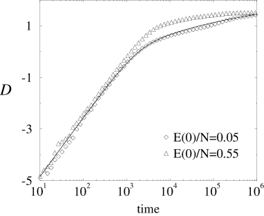
Figure 2: Symbols represent ${\cal D}$ versus time for an FPU chain with $N=256$, $\gamma=0.05$ and with free–end (a) and fixed–end (b) boundary conditions. Solid line is the plot of formula (11).

In figure 2 we plot ${\cal D}$ vs time for two chains of size $N=256$ with free–end and fixed–end BC. In both cases no evidence of stretched exponential decay is found. The curves follow to a very good extent the characteristic trend of the linear model (see equation (11) ). This remarkable observation can be interpreted by the following arguments. First of all, an approximate description in terms of an effective harmonic model with energy–dependent renormalized frequencies proved to succesfully account for a number of equilibrium properties of the FPU chain [10, 11]. If we assume that the energy extraction rate is slow enough for the system to evolve in a quasi–static fashion, we may reasonably expect that a similar scenario as the one described for the harmonic case emerges. Second, the harmonic approximation becomes increasingly accurate as time elapses, simply because more and more energy is extracted from the system by the reservoir.

Actually, the energy–dependent corrections to the linear spectrum only induce in the energy decay curves small deviations from the linear case. Indeed, a closer inspection of figure 2 reveals that changing the initial energy density $E(0)/N$ only affects the first crossover region, for both free–end and fixed–end BC.

A dramatic deviation from the linear–like behaviour emerges however at a later stage, when the localization of energy sets in. We observe the spontaneous birth of breathers, analogous to what reported in ref [5]. This process pins the energy at some sites in the chain, thus forcibly causing a further slowing down of the energy decay. Nevertheless, we note that this can hardly be detected from the energy decay curves, which are mainly determined by the relaxation of the Fourier modes. On the other hand, localization is clearly revealed by plotting the parameter ${\cal L}$ defined by formula (5) (see figure 3). Remarkably, in the free–end chain we have observed spontaneous excitation of breathers for all the performed numerical experiments. On the contrary, localization turns out to be strongly inhibited for the fixed–end chain. As a matter of fact, we have observed it in a very small fraction (say $5\%$) of the numerical experiments. Moreover, the degree of localization (i.e. the asymptotic value of ${\cal L}$) depends on the initial energy.

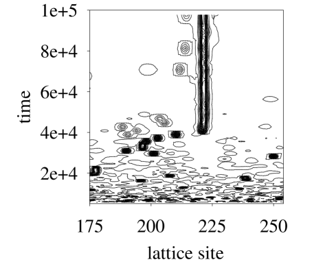
Figure 4: FPU chain with $N=256$. (a) Lower panel: log-log plot of the first power–law portion of the energy decay curves. Best fits (solid lines) give exponents $-0.51$ and $-0.53$ for $E(t)/E(0)=0.05$ and $1.0$, respectively. The upper panels show the trend of the localization parameter ${\cal L}$ for both cases in the same time domain. (b) Space–time contour plot of the symmetrized site energies for $E(t)/E(0)=1.0$. The figure shows a close–up in the region of the chain where the breather develops.

The pathway to localization is similar to the one described in ref [3], whereby one breather is formed from a collection of short–lived localized vibrations that eventually merge together. The situation is shown for a typical simulation in figure 4 (b) in the form of a space–time contour plot of the symmetrized site energies. The localized modes that emerge out of the relaxation process are very similar to the ones that originate from the modulational instability of the zone–boundary modes in the hamiltonian system [3, 12]. This is seen by looking at the displacement and velocity pattern of the particles and their spatial spectra. Moreover, the localized objects are seen to either stay fixed or move with a definite velocity [12]. As a consequence they may collide with the boundaries, thereby loosing some energy. However, these losses turn out to be tiny, not only because the interaction with the reservoirs are quasi–elastic (at least for $\gamma\ll 1$) but also because the breather velocity is typically smaller than the sound speed.

To further confirm that the damped system supports breathers similar to the ones known from the hamiltonian case, we have performed the following numerical experiment. A pattern corresponding to a zero–velocity DB solution in a lattice of size $N=256$ has been computed numerically within the framework of the rotating wave approximation (RWA) [13]. This solution has then been used as the initial condition for the evolution equations (1). The results are summarized in figure 5, where we plot the energy decay curve alongside with a snapshot of the lattice displacements at the end of the simulation and the localization parameter. The dissipation acts effectively in eliminating the vibrational junk radiating from the approximate solution and stabilizing it. The extremely slow decay of the breather energy (see lower panel in figure 5) is presumably due to anelastic scattering with small amplitude plane waves [14].

We can understand what difference the BC make for localization by recalling what we have learnt from the harmonic chain together with the known effect of modulational instability of the zone–boundary modes [12, 15]. In fact, we see that the main difference between the two cases is in the relaxation rates of the Fourier modes (see equation (8) and (9)). This implies that in the free–end system the long–wavelength modes quickly disappear from the lattice, leaving there just the long–lived zone–boundary ones. This explains why modulational instability is so effective for the formation of breathers. On the contrary, the “longevity” of the long–wavelength modes in the fixed–end chain spoils such instability process, unless a very big energy fluctuation overcomes the other effect providing an alternative localization pathway.

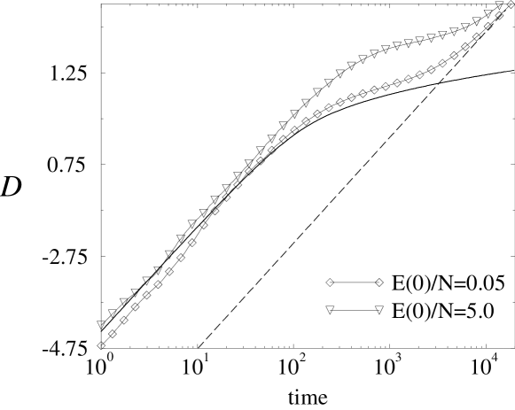
Figure 6: Symbol represent ${\cal D}$ versus time for an FPU chain with $N=16$ and fixed–end boundary conditions. Solid and dashed lines are plots of formula (11) and of the law $\exp(-2t/\tau_{N-1})$, with $\tau_{N-1}=N(N+1)^{2}/2\pi^{2}\gamma$, respectively.

As already pointed out, only the long–term portion of the energy relaxation curves is affected by localization. Indeed, in the absence of breathers, the energy slowly drifts back to an exponential law. This is clearly seen in figure 6, where we plot ${\cal D}$ versus time for a fixed-end FPU chain. In order to better illustrate this point, we show in figure 4 (a) two fits to the first power–law portion of the energy decay curves for two values of the initial energy. In the lower energy simulation localization has not yet occurred. On the contrary, at the higher energy, the same portion of the curve corresponds to arousal of localization (see also figure 4 (b)). This is reflected in the trend of ${\cal L}$ for the two cases. We see that the trends of ${\cal D}(t)$ are clearly indistinguishable in the two cases, making emergence of localization difficult to spot from the energy decay curves.

5 Conclusions

We have analysed the energy relaxation of chains of atoms with linear and FPU interaction potential by applying a damping term at the chain boundaries. Both free–end and fixed–end conditions have been considered. We have shown that also the simple linear system is characterized by nontrivial relaxation features, that are determined by the interplay of different relaxation time scales. These are characteristic for each Fourier mode, which relaxes exponentially in time with a decay rate depending on its wavenumber. In particular, we have derived a two–crossover picture of the decay process. More precisely, for $t>\tau_{0}=N/2\gamma$ the initial exponential behaviour slows down to an inverse square–root law. At a later stage ($t>\tau_{\scriptscriptstyle N-1}\propto N^{3}/\gamma$) the system comes back to an exponential decay with a relaxation rate twice the one of the slowest Fourier mode. Furthermore, the first crossover is independent of the BC, while the second one depends on them.

We have analysed the nonlinear system under the same conditions and found that the behaviour is almost concident with the linear case, provided the energy extraction rate is not too fast. Noticeably, our data are not compatible with a stretched–exponential relaxation. As a side but important result, we clarify why the fixed–end FPU chain does not display spontaneous localization as a product of the energy extraction process. This is because the long–wavelength modes of the fixed–end chain at equilibrium are characterized by high amplitudes and vanishing relaxation rates, that are proportional to $\gamma/N^{3}$ . As a result, the modulational instability of the short–wavelength modes is not effective in producing localized vibrations and the energy decay behaviour of the fixed–end FPU chain is practically equivalent to the linear case.

The dependence of the characteristic time scales on the system size stems from the choice of the damping matrix $\Gamma$. More generally, if one fixes the fraction $f$ of the damped particles, the first crossover time $\tau_{0}$ becomes independent of $N$ (and inversely proportional to $f$), while the second one $\tau_{\scriptscriptstyle N-1}$ is still expected to scale as $N^{3}$.

In summary, we have brought forward the intrinsic complexity of spontaneous breather excitation in spatially extended nonlinear systems. In particular, we have illustrated the importance of the system size and of the boundary conditions for such studies.

We want also to observe that the above conclusions hold for 1D nonlinear chains, where relaxation produces localization of the energy for arbitrarily small initial energy. The situation may be significantly different in 2D due to the presence of an energy threshold for breather solutions [16]. Preliminary numerical studies of the 2D FPU model seem to confirm such expectations. This point certainly deserves deeper investigations, that might provide further insight on the relevance of breathers as spontaneous excitations emerging from a relaxation dynamics in nonlinear lattices.

Appendix A

In this Appendix we report the details of the calculation of the damping rates for the harmonic lattice. In matrix notation the equations of motion read

$$\ddot{u}=Ku-\Gamma\dot{u}$$ (14)

where $u$ is the column vector $(u_{0},u_{1},\dots u_{N-1})$, while $K$ is the matrix

$$K_{pp^{\scriptscriptstyle\prime}}=\frac{k_{2}}{m}\left[\delta_{p^{\scriptscriptstyle\prime},p+1}+\delta_{p^{\scriptscriptstyle\prime},p-1}-2\delta_{p^{\scriptscriptstyle\prime},p}\right]$$ (15)

The top and bottom diagonal elements of matrix $K$ are defined as $K_{00}=K_{(N-1),(N-1)}=-k_{2}/m$ for free–end BC, while definition  (15) applies to fixed–end BC. The eigenvectors of the hamiltonian problem satisfy the orthonormality conditions

$$\eqalign{(\eta^{\alpha},\eta^{\alpha^{\scriptscriptstyle\prime}})=\sum_{p=0}^{N-1}\eta^{\alpha}_{p}\eta^{\alpha^{\scriptscriptstyle\prime}}_{p}=\delta_{\alpha,\alpha^{\scriptscriptstyle\prime}}\\ (\eta^{\alpha},K\eta^{\alpha^{\scriptscriptstyle\prime}})=\sum_{p,p^{\scriptscriptstyle\prime}=0}^{N-1}\eta^{\alpha}_{p}K_{pp^{\scriptscriptstyle\prime}}\eta^{\alpha^{\scriptscriptstyle\prime}}_{p^{\scriptscriptstyle\prime}}=-\omega_{\alpha}^{2}\delta_{\alpha,\alpha^{\scriptscriptstyle\prime}},}$$ (18)

By substituting expression (6) in equation (14), we get

$$\sum_{\alpha=0}^{N-1}[\ddot{c}_{\alpha}(t)-\omega_{\alpha}^{2}c_{\alpha}(t)-2i\omega_{\alpha}\dot{c}_{\alpha}(t)]e^{-i\omega_{\alpha}t}\eta^{\alpha}_{p}-\sum_{\alpha=0}^{N-1}c_{\alpha}(t)e^{-i\omega_{\alpha}t}\sum_{p^{\scriptscriptstyle\prime}=0}^{N-1}K_{pp^{\scriptscriptstyle\prime}}\eta^{\alpha}_{p^{\scriptscriptstyle\prime}}=$$

$$-\sum_{\alpha=0}^{N-1}[\dot{c}_{\alpha}(t)-i\omega_{\alpha}c_{\alpha}(t)]e^{-i\omega_{\alpha}t}\sum_{p^{\scriptscriptstyle\prime}=0}^{N-1}\Gamma_{pp^{\scriptscriptstyle\prime}}\eta^{\alpha}_{p^{\scriptscriptstyle\prime}}.$$

By taking the scalar product of the latter equation with $\eta^{\alpha^{\scriptscriptstyle\prime}}$ and recalling the orthonormality conditions contained in (18), we are led to the system of equations

$$\ddot{c}_{\alpha}(t)-2i\omega_{\alpha}\dot{c}_{\alpha}(t)=-\sum_{\alpha^{\scriptscriptstyle\prime}=0}^{N-1}[\dot{c}_{\alpha^{\scriptscriptstyle\prime}}(t)-i\omega_{\alpha^{\scriptscriptstyle\prime}}c_{\alpha^{\scriptscriptstyle\prime}}(t)]\,\Gamma^{\alpha\alpha^{\scriptscriptstyle\prime}}e^{-i(\omega_{\alpha^{\scriptscriptstyle\prime}}-\omega_{\alpha})t},$$ (19)

where

$$\Gamma^{\alpha\alpha^{\scriptscriptstyle\prime}}=(\eta^{\alpha},\Gamma\,\eta^{\alpha^{\scriptscriptstyle\prime}})=\sum_{p,p^{\scriptscriptstyle\prime}=0}^{N-1}\eta^{\alpha}_{p}\Gamma_{pp^{\scriptscriptstyle\prime}}\eta^{\alpha^{\scriptscriptstyle\prime}}_{p^{\scriptscriptstyle\prime}}$$ (20)

We can obtain approximate solutions of system (19) by means of a perturbative series of the form

$$c_{\alpha}(0)=c_{\alpha}^{[0]}(t)+c_{\alpha}^{[1]}(t)+c_{\alpha}^{[2]}(t)+\dots,$$

where $c_{\alpha}^{[1]}(t)$, $c_{\alpha}^{[2]}(t)$, $\dots$ are first order, second order amplitudes, and so on, in the perturbation parameter $\gamma$. We can then use the usual iterative procedure. If we assume that at $t=0$ only the mode $\alpha=\bar{\alpha}$ is populated, we can approximate $c_{\alpha}(t)=\delta_{\alpha,{\bar{\alpha}}}$ (independent of $t$) in the right–hand side of equation (19) and then integrate to get $c_{\alpha}^{[1]}(t)$. The procedure can be repeated for obtaining $c_{\alpha}^{[2]}(t)$, etc. For the first order approximation we obtain the following equation

$$\ddot{c}_{\alpha}(t)-[2i\omega_{\alpha}-\Gamma^{\alpha\alpha}]\dot{c}_{\alpha}(t)-i\omega_{\alpha}\Gamma^{\alpha\alpha}c_{\alpha}(t)=0,$$

which is readily integrated, yielding expression (7).

To calculate the matrix elements $\Gamma^{\alpha\alpha}$, we need the explicit expression of the eigenvectors of the unperturbed problem, which are

$$\eta^{\alpha}_{p}=\sqrt{\frac{2}{N}}\cos\left[q_{\alpha}\left(p+\frac{1}{2}\right)\right],\ \ \ \ q_{\alpha}=\frac{\alpha\pi}{N},\ \ \ \ \alpha=0,1\dots N-1$$ (21)

for the free–end chain, and

$$\eta^{\alpha}_{p}=\sqrt{\frac{2}{N}}\sin\left[q_{\alpha}(p+1)\right],\ \ \ \ q_{\alpha}=\frac{(\alpha+1)\pi}{N+1},\ \ \ \ \alpha=0,1\dots N-1$$ (22)

for the fixed–end one. By inserting these expressions in equation (20), one can easily obtain equation (8) and equation (9).

References

Figure captions

Figure 3: The localization parameter ${\cal L}$ vs time for an FPU chain of size $N=256$ with free–end (a) and fixed–end (b) boundary conditions.

Figure 5: Plots of an RWA solution relaxing in an $N=256$ chain. Lower panel: normalized energy vs time. Upper left panel: snapshot of the atomic displacements at $t=5\cdot 10^{6}$. Upper right panel: the localization parameter ${\cal L}$ vs time.

References

- [1] Flach S, Willis C R, 1998 Phys. Rep., 295, 181
- [2] Aubry S, MacKay R S, 1994 Nonlinearity 7, 1623
- [3] Cretegny T Dauxois T Ruffo S and Torcini A 1998 Physica D 121 106
- [4] Lepri S, Livi R and Politi A 1998 Europhys. Lett. 43 271
- [5] Tsironis G P and Aubry S 1996 Phys. Rev. Lett. 77 (26) 5225
- [6] Bikaki A, Voulgarakis N K Aubry S and Tsironis G P 1999 Phys. Rev. E 59 (1) 1234
- [7] Bunde A et al, 1998 Phil. Mag. B 77 (5) 1323 and references therein
- [8] Palmer R G Stein D L Abrahams E and Anderson P W 1984 Phys. Rev. Lett. 53 (10) 958
- [9] Sanz–Serna J M and Calvo M P 1994 Numerical Hamiltonian Problems (London: Chapman & Hall)
- [10] Alabiso C Casartelli M Marenzoni P 1995 J. Stat. Phys 79 451
- [11] Lepri S 1998 Phys. Rev. E 58 (6) 7165
- [12] Kosevich Yu A and Lepri S 2000 Phys. Rev. B 61 (1) 299
- [13] Sievers A J and Takeno S 1988 Phys. Rev. Lett. 61 970
- [14] Johansson M and Aubry S 2000 Phys. Rev. E 61 5864
- [15] Daumont I Dauxois T and Peyrard M 1997 Nonlinearity 10 617
- [16] Flach S Kladko K and MacKay R S 1997 Phys. Rev. Lett. 78 1207