Determination of the threshold of the break-up of invariant tori in a class of three frequency Hamiltonian systems

Abstract

We consider a class of Hamiltonians with three degrees of freedom that can be mapped into quasi-periodically driven pendulums. The purpose of this paper is to determine the threshold of the break-up of invariant tori with a specific frequency vector. We apply two techniques : the frequency map analysis and renormalization-group methods. The renormalization transformation acting on a Hamiltonian is a canonical change of coordinates which is a combination of a partial elimination of the irrelevant modes of the Hamiltonian and a rescaling of phase space around the considered torus. We give numerical evidence that the critical coupling at which the renormalization transformation starts to diverge is the same as the value given by the frequency map analysis for the break-up of invariant tori. Furthermore, we obtain by these methods numerical values of the threshold of the break-up of the last invariant torus.

1 Introduction

For Hamiltonian systems, the persistence of invariant tori influences the global properties of the dynamics. The study of the break-up of invariant tori is thus an important issue to understand the onset of chaos. For two degrees of freedom, there are several numerical methods to determine the threshold of the break-up of invariant tori : for instance, Greene’s criterion [1], obstruction method [2], converse KAM [3, 4], frequency map analysis [5, 6, 7, 8], or renormalization-group methods [9, 10, 11].
In this article, we propose to compute this threshold for a one-parameter family of Hamiltonians with three degrees of freedom and for a specific frequency vector, by two techniques : by frequency map analysis and by renormalization. The frequency map analysis is valid for any dimension, and has been applied to systems with a large number of degrees of freedom [5]. The set-up of renormalization-group transformations is also possible for any dimensions in the framework of Ref. [12], but only systems with two degrees of freedom have been investigated numerically.
We describe the renormalization-group transformation and we implement it numerically for the spiral mean torus. The result is that the values of the critical coupling given by the renormalization coincide up to numerical precision with the thresholds of the break-up of the spiral mean torus (of dimension 3) given by frequency map analysis. The two methods we compare are completely independent, both conceptually and in their practical realizations. The frequency map analysis is based on the analysis of trajectories, while the renormalization is based on a criterion of convergence of a sequence of canonical transformations.
We conjecture, on the basis of this numerical result, that the renormalization-group transformation converges up to the critical surface (the set of Hamiltonians where the torus of the given frequency is critical, i.e. at the threshold of its break-up), at least in a region of the critical surface of the Hamiltonian space where critical couplings are small enough (in order that the elimination procedure is well-defined [13]).

We consider a class of Hamiltonians with three degrees of freedom written in terms of actions $\bm{A}=(A_{1},A_{2},A_{3})\in{\mathbb{R}}^{3}$ and angles $\bm{\varphi}=(\varphi_{1},\varphi_{2},\varphi_{3})\in{\mathbb{T}}^{3}$ (the 3-dimensional torus parametrized, e.g., by $[0,2\pi]^{3}$)

$$H_{\varepsilon}(\bm{A},\bm{\varphi})=H_{0}(\bm{A})+\varepsilon V(\bm{\varphi}),$$ (1)

where $\varepsilon$ denotes the coupling parameter. In this article, we consider the particular class of models for which the integrable part $H_{0}$ is given by

$$H_{0}({\bm{A}})={\bm{\omega}}_{0}\cdot{\bm{A}}+\frac{1}{2}({\bm{\Omega}}\cdot{\bm{A}})^{2},$$ (2)

where $\bm{\omega}_{0}$ is the frequency vector of the considered invariant torus, and $\bm{\Omega}$ is another constant vector non-parallel to $\bm{\omega}_{0}$. We suppose that $\bm{\omega}_{0}$ is incommensurate, i.e. there is no nonzero integer vector $\bm{\nu}$ such that $\bm{\omega}_{0}\cdot\bm{\nu}=0$.
Since the quantity $\bm{\omega}_{0}^{\perp}\cdot\bm{\varphi}$ is conserved (where $\bm{\omega}_{0}^{\perp}$ denotes a vector orthogonal to $\bm{\Omega}$ and to $\bm{\omega}_{0}$), one can show (even if $\bm{\omega}_{0}^{\perp}\cdot\bm{\varphi}$ is not a function on the three-dimensional torus) that this model (1)-(2) is intermediate between two and three degrees of freedom; in appropriate coordinates it can be interpreted as one degree of freedom driven by a multi-periodic force with incommensurate frequencies $\bm{\omega}_{0}$. In particular, invariant tori in this intermediate model act as barriers in phase space (limiting the diffusion of trajectories) in a similar way as for two degrees of freedom Hamiltonian systems. We analyze in this article the break-up of invariant tori with spiral mean frequencies for this particular type of models, by choosing a special form of the perturbation (see section 3), such that the model is equivalent to a pendulum driven by two periodic forces with incommensurate frequencies. The method is however applicable to any perturbation and to the case of full three degrees of freedom [12, 19].
We are interested in the stability of the torus with frequency vector $\bm{\omega}_{0}$. For the unperturbed Hamiltonian $H_{0}$, this torus is located at $\bm{A}=\bm{0}$. Kolmogorov-Arnold-Moser (KAM) theorems were proven for Hamiltonians (1) provided that $\bm{\omega}_{0}$ satisfies a Diophantine condition [14]. This theorem shows the existence of the torus with frequency vector ${\bm{\omega}}_{0}$ for a sufficiently small and smooth perturbation $\varepsilon V$. The invariant torus is a small deformation of the unperturbed one. The existence of the torus outside the perturbative regime is still an open question even if efforts have been made to increase lower bounds for specific models (for a two dimensional model, see Ref. [15, 16]). Conversely, for sufficiently large values of the coupling parameter, it has been shown that the torus does no longer exist [3, 4]. The aim of this paper is to determine $\varepsilon_{c}$ such that $H_{\varepsilon}$ has a smooth invariant torus of the given frequency for $|\varepsilon|<\varepsilon_{c}$, and does not have this invariant torus for $|\varepsilon|>\varepsilon_{c}$.
The invariant torus we study (named the spiral mean torus) has the frequency vector

$${\bm{\omega}}_{0}=(\sigma^{2},\sigma,1),$$

where $\sigma$ is the spiral mean, i.e. the real root of $\sigma^{3}=\sigma+1$ ($\sigma\approx 1.3247$). From some of its properties, $\sigma$ plays a similar role as the golden mean in the two degrees of freedom case [17]. The analogy comes from the fact that one can generate rational approximants by iterating a single unimodular matrix $N$. In what follows, we call resonance an element of the sequence $\{{\bm{\nu}}_{k}=N^{k-1}{\bm{\nu}}_{1},k\geq 1\}$ where ${\bm{\nu}}_{1}=(1,0,0)$ and

$$N=\left(\begin{array}[]{ccc}0&0&1\\ 1&0&0\\ 0&1&-1\end{array}\right).$$

The word resonance refers to the fact that the small denominators ${\bm{\omega}}_{0}\cdot{\bm{\nu}}_{k}$ appearing in the perturbation series or in the KAM iteration, tend to zero geometrically as $k$ increases (${\bm{\omega}}_{0}\cdot{\bm{\nu}}_{k}=\sigma^{3-k}\to 0\mbox{ as }k\to\infty$). We notice that $\bm{\omega}_{0}$ is an eigenvector of $\tilde{N}$, where $\tilde{N}$ denotes the transposed matrix of $N$. One can prove [12] that $\bm{\omega}_{0}$ satisfies a Diophantine condition of the form :

$$|{\bm{\omega}}_{0}\cdot{\bm{\nu}}|>c|{\bm{\nu}}|^{-2},$$

where $|{\bm{\nu}}|=(|\nu_{1}|^{2}+|\nu_{2}|^{2}+|\nu_{3}|^{2})^{1/2}$, and $c\approx 0.6$.

2 Renormalization-group transformation

The renormalization transformations are defined for a fixed frequency vector $\bm{\omega}_{0}$, and contain a partial elimination of the irrelevant modes (the non-resonant part) of the perturbation, and a rescaling of phase space. The elimination of irrelevant modes is performed by iterating a change of coordinates as in KAM theory. We remark that other perturbative techniques can be used instead, leading to similar results. The rescaling of phase space combines a shift of the resonances, a rescaling of time, and a rescaling of the actions. The aim is to change the scale of the actions to a smaller one (and a longer time scale). This renormalization can be thought as a microscope in phase space. The non-resonant modes are the ones which affect the motion at short time scales, and can be dealt with averaging methods. We define the non-resonant modes to be the ones that satisfy the inequality

$$|\bm{\omega}_{0}\cdot\bm{\nu}|>\frac{1}{\sqrt{2}}|\bm{\omega}_{0}||\bm{\nu}|.$$ (3)

This set of modes, denoted $I^{-}$, is the interior of a cone around the $\bm{\omega}_{0}$-direction in the space of 3-dimensional vectors, with angle $\pi/4$. We define the resonant modes as the Fourier modes which do not satisfy the condition (3), i.e. this set, denoted $I^{+}$, is the complement of $I^{-}$ in ${\mathbb{Z}}^{3}$. Since $\bm{\nu}_{k}$ does not satisfy Eq. (3) for $k\geq 1$, $I^{+}$ contains the resonances that produce small denominators in the perturbation series or in the KAM theory. The “frequency cut-off” (between resonant and non-resonant modes) restricts the Fourier modes that can be eliminated in one renormalization step, without running into small denominator problems (the non-resonant modes). As it is common with cut-offs, there is not a single “natural” choice. More generally, other choices in the splitting of $\{e^{i\bm{\nu}\cdot\bm{\varphi}}\}$ into resonant and non-resonant modes should lead to the same results provided, e.g., that the ratio $|{\bm{\nu}}|/|{\bm{\omega}}_{0}\cdot{\bm{\nu}}|$ is bounded on $I^{-}$, and that the shift of the resonances contracts non-zero vectors ${\bm{\nu}}$ in $I^{+}$ and maps them into $I^{-}$ after a finite number of iterations of the transformation [11, 12].

The transformation, acting on a Hamiltonian $H$ of the form

$$H(\bm{A},\bm{\varphi})=H_{0}(\bm{A})+V(\bm{\Omega}\cdot\bm{A},\bm{\varphi}),$$ (4)

where $H_{0}$ is given by Eq. (2), combines four steps:
(1) We shift the resonances ${\bm{\nu}}_{k+1}\mapsto{\bm{\nu}}_{k}$: We require that the new angles $\bm{\varphi}^{\prime}$ satisfy

$$\cos(\bm{\nu}_{k+1}\cdot\bm{\varphi})=\cos(\bm{\nu}_{k}\cdot\bm{\varphi}^{\prime}),$$

for $k\geq 1$. This is performed by the linear canonical transformation

$$(\bm{A},\bm{\varphi})\mapsto(\bm{A}^{\prime},\bm{\varphi}^{\prime})=(N^{-1}\bm{A},\tilde{N}\bm{\varphi}).$$

Since $N$ is an integer matrix with determinant one, this transformation preserves the ${\mathbb{T}}^{3}$-structure of the angles. We notice that the resonance $\bm{\nu}_{1}$ is changed into $\bm{\nu}_{0}=(0,1,1)$ which satisfies the condition (3), i.e. it is a non-resonant mode : Some of the resonant modes are turned into non-resonant ones by this linear transformation.
This step changes the frequency ${\bm{\omega}}_{0}$ into $\tilde{N}{\bm{\omega}}_{0}=\sigma^{-1}{\bm{\omega}}_{0}$ (since ${\bm{\omega}}_{0}$ is an eigenvector of $\tilde{N}$ by construction), and the vector $\bm{\Omega}$ into $\tilde{N}\bm{\Omega}$. In order to keep a unit norm, we define the image of $\bm{\Omega}$ by

$$\bm{\Omega}^{\prime}=\frac{\tilde{N}\bm{\Omega}}{\|\tilde{N}\bm{\Omega}\|}.$$ (5)

(2) We rescale the energy (or equivalently time) by a factor $\sigma$ (i.e. we multiply the Hamiltonian by $\sigma$), in order to keep the frequency fixed at ${\bm{\omega}}_{0}$.
(3) We rescale the actions :

$$H^{\prime}({\bm{A}},{\bm{\varphi}})=\lambda H\left(\frac{{\bm{A}}}{\lambda},{\bm{\varphi}}\right),$$

such that the mean-value of the coefficient of the quadratic term in $H^{\prime}$ is equal to $(\bm{\Omega}^{\prime}\cdot\bm{A})^{2}/2$. This normalization condition is essential for the convergence of the transformation. After Steps 1, 2 and 3, the Hamiltonian expressed in the new variables is

$$H^{\prime}(\bm{A},\bm{\varphi})=\lambda\sigma H\left(\frac{1}{\lambda}N\bm{A},\tilde{N}^{-1}\bm{\varphi}\right).$$ (6)

For $H$ given by Eq. (4), this expression becomes

$$H^{\prime}(\bm{A},\bm{\varphi})=\bm{\omega}_{0}\cdot\bm{A}+\frac{\sigma}{2\lambda}\|\tilde{N}\bm{\Omega}\|^{2}(\bm{\Omega}^{\prime}\cdot\bm{A})^{2}+\lambda\sigma V\left(\frac{\|\tilde{N}\bm{\Omega}\|}{\lambda}\bm{\Omega}^{\prime}\cdot\bm{A},\tilde{N}^{-1}\bm{\varphi}\right).$$ (7)

Thus the choice of the rescaling in the actions (Step 3) is

$$\lambda=\sigma\|\tilde{N}\bm{\Omega}\|^{2}(1+2\langle V^{(2)}\rangle),$$ (8)

where $\langle V^{(2)}\rangle$ denotes the coefficient of the mean-value of the quadratic part, in the representation :

$$V(\bm{\Omega}^{\prime}\cdot\bm{A},\bm{\varphi})=\sum_{j\geq 0}V^{(j)}(\bm{\varphi})(\bm{\Omega}^{\prime}\cdot\bm{A})^{j}.$$

(4) We perform a near-identity canonical transformation ${\mathcal{U}}_{H}$ that eliminates completely the non-resonant part of the perturbation in $H^{\prime}$. This transformation satisfies the following equation :

$${\mathbb{I}}^{-}\left(H^{\prime}\circ{\mathcal{U}}_{H}\right)=0,$$ (9)

where ${\mathbb{I}}^{-}$ denotes the projection operator on the non-resonant modes acting on a Hamiltonian $H$ as

$${\mathbb{I}}^{-}H(\bm{A},\bm{\varphi})=\sum_{\bm{\nu}\in I^{-}}H_{\bm{\nu}}(\bm{A})e^{i\bm{\nu}\cdot\bm{\varphi}}.$$ (10)

Equation (9) is solved by a Newton method. We iterate a change of coordinates as in KAM theory that reduces the non-resonant modes of the perturbation from $\varepsilon$ to $\varepsilon^{2}$. One step of the elimination is performed by a Lie transformation ${\mathcal{U}}_{S}:({\bm{A}},{\bm{\varphi}})\mapsto({\bm{A}}^{\prime},{\bm{\varphi}}^{\prime})$, generated by a function $S(\bm{A},\bm{\varphi})$. The expression of a Hamiltonian $H$ in the new coordinates is given by

$$H\circ{\mathcal{U}}_{S}=\exp(\hat{S})H\equiv H+\{S,H\}+\frac{1}{2!}\{S,\{S,H\}\}+\cdots,$$ (11)

where $\{\,,\,\}$ is the Poisson bracket between two scalar functions of the actions and angles:

$$\{f,g\}=\frac{\partial f}{\partial\bm{\varphi}}\cdot\frac{\partial g}{\partial\bm{A}}-\frac{\partial f}{\partial\bm{A}}\cdot\frac{\partial g}{\partial\bm{\varphi}},$$ (12)

and the operator $\hat{S}$ is defined as $\hat{S}H\equiv\{S,H\}$. The generating function $S$ is chosen such that the order $\varepsilon$ of the non-resonant part of the perturbation vanishes. We construct recursively a series of Hamiltonians $H_{n}$, starting with $H_{1}=H^{\prime}$, such that the limit $H_{\infty}$ is canonically conjugate to $H^{\prime}$ but does not contain non-resonant modes, i.e. ${\mathbb{I}}^{-}H_{\infty}=0$. One step of this elimination procedure, $H_{n}\mapsto H_{n+1}$, is done by applying a change of coordinates ${\mathcal{U}}_{n}$ such that the order of the non-resonant modes of $H_{n+1}=H_{n}\circ{\mathcal{U}}_{n}$ is $\varepsilon_{n}^{2}$, where $\varepsilon_{n}$ denotes the order of the non-resonant modes of $H_{n}$. At the $n$-th step, the order of the non-resonant modes of $H_{n}$ is $\varepsilon_{0}^{2^{n-1}}$, where $\varepsilon_{0}$ is the order of the non-resonant modes of $H^{\prime}$. If this procedure converges, it defines a canonical transformation ${\mathcal{U}}_{H}={\mathcal{U}}_{1}\circ{\mathcal{U}}_{2}\circ\cdots\circ{\mathcal{U}}_{n}\circ\cdots$, such that the final Hamiltonian $H_{\infty}=H^{\prime}\circ{\mathcal{U}}_{H}$ does not contain any non-resonant mode.
The specific implementation of one step of this elimination procedure will be described more explicitly in the next sections. We will discuss two versions of this transformation : The first one is a renormalization for Hamiltonians in power series in the actions, and the second one is a slightly different version which eliminates only the non-resonant modes of the constant and linear part in the actions of the rescaled Hamiltonian $H^{\prime}$, and which allows us to define a renormalization within a space of quadratic Hamiltonians in the actions, following Thirring’s approach of the KAM theorem [18].
It has been proven in Ref. [12] that, for a sufficiently small non-resonant part of the perturbation, the transformation ${\mathcal{U}}_{H}$ is a well-defined canonical transformation such that a Hamiltonian expressed in these new coordinates does not have non-resonant modes. The domain of definition of ${\mathcal{U}}_{H}$ has been extended to some non-perturbative domain in Ref. [13].
Concerning the quadratic case, we lack at this moment a theoretical background to prove an analogous theorem. The convergence of the elimination procedure in both cases outside the perturbative regime ($\varepsilon$ small) is observed numerically.

In summary, the renormalization-group transformations we define act as follows : First, some of the resonant modes of the perturbation are turned into non-resonant modes by a frequency shift and a rescaling. Then, a KAM-type iteration eliminates these non-resonant modes, while slightly changing the resonant modes.

2.1 Renormalization scheme for Hamiltonians in power series in the actions

We define in this section, one step of the elimination of the non-resonant modes of the rescaled Hamiltonian $H^{\prime}$. The renormalization transformation acts on the following family of Hamiltonians

$$H(\bm{A},\bm{\varphi})=\bm{\omega}_{0}\cdot\bm{A}+\sum_{j=0}^{\infty}V^{(j)}(\bm{\varphi})(\bm{\Omega}\cdot\bm{A})^{j},$$ (13)

with $\langle V^{(0)}\rangle=0$. We suppose that $\langle V^{(2)}\rangle$ is nonzero (in order to have a twist direction in the actions). The approximations involved in this transformation are of two types : we truncate the Fourier series of the functions $V^{(j)}$, i.e. we approximate a scalar function $f$ of the angles by

$$f^{[\leq L]}(\bm{\varphi})=\sum_{\bm{\nu}\in{\mathcal{C}}_{L}}f_{\bm{\nu}}e^{i\bm{\nu}\cdot\bm{\varphi}},$$ (14)

where ${\mathcal{C}}_{L}=\{\bm{\nu}=(\nu_{1},\nu_{2},\nu_{3})\in{\mathbb{Z}}^{3}\left|\max_{i}|\nu_{i}|\leq L\right.\}$, and we also neglect all the terms of order $O\left((\bm{\Omega}\cdot\bm{A})^{J+1}\right)$ that are produced by the transformation.
One step of the elimination procedure $H\mapsto\tilde{H}=H\circ{\mathcal{U}}_{S}$ is constructed as follows : We consider that $V^{(j)}$ depends on a small parameter $\varepsilon$, such that ${\mathbb{I}}^{-}V^{(j)}$ is of order $\varepsilon$. We define $H_{0}$, the integrable part of $H$ as

$$H_{0}(\bm{A})=\bm{\omega}_{0}\cdot\bm{A}+\langle V^{(2)}\rangle(\bm{\Omega}\cdot\bm{A})^{2},$$ (15)

and the perturbation of $H_{0}$ is denoted $V^{\prime}=H-H_{0}=V-\langle V^{(2)}\rangle(\bm{\Omega}\cdot\bm{A})^{2}$. In order to eliminate the non-resonant modes of $V^{(j)}$ to the first order in $\varepsilon$, we perform a Lie transformation ${\mathcal{U}}_{S}:(\bm{A},\bm{\varphi})\mapsto(\bm{A}^{\prime},\bm{\varphi}^{\prime})$ generated by a function $S$ of order $\varepsilon$ and of the form

$$S(\bm{A},\bm{\varphi})=i\sum_{j=0}^{J}Y^{(j)}(\bm{\varphi})(\bm{\Omega}\cdot\bm{A})^{j}+a\bm{\Omega}\cdot\bm{\varphi}.$$ (16)

The first terms of $\tilde{H}$ are $H_{0}+V^{\prime}+\{S,H_{0}\}+\{S,V^{\prime}\}+O(\varepsilon^{2})$. The function $S$ is determined by imposing that the order $\varepsilon$ vanishes :

$${\mathbb{I}}^{-}\{S,H_{0}\}+{\mathbb{I}}^{-}V^{\prime}+{\mathbb{I}}^{-}\{S,{\mathbb{I}}^{+}V^{\prime}\}=0.$$ (17)

This condition determines the non-resonant modes of $S$. For the resonant ones, we choose ${\mathbb{I}}^{+}S=0$. Thus we notice that the mean value of $\{S,{\mathbb{I}}^{+}V^{\prime}\}$ is zero. The constant $a$ eliminates the linear term in the $(\bm{\Omega}\cdot\bm{A})$-variable, $\langle V^{(1)}\rangle$, by requiring that $\langle\{S,H_{0}\}\rangle+\langle V^{(1)}\rangle\bm{\Omega}\cdot\bm{A}=0$:

$$a=-\frac{\langle V^{(1)}\rangle}{2\Omega^{2}\langle V^{(2)}\rangle}.$$ (18)

We solve Eq. (17) by a Newton method with an initial condition which satisfies ${\mathbb{I}}^{-}\{S,H_{0}\}+{\mathbb{I}}^{-}V=0$, since ${\mathbb{I}}^{+}V^{\prime}$ is expected in general to be small. Then we compute $\tilde{H}=H\circ{\mathcal{U}}_{S}$ by calculating recursively the Poisson brackets $\hat{S}^{k}H=\hat{S}\hat{S}^{k-1}H$, for $k\geq 1$. Denoting $H_{k}=\hat{S}^{k}H$, $\tilde{H}$ becomes

$$\tilde{H}=\sum_{k=0}^{\infty}\frac{H_{k}}{k!}.$$ (19)

2.2 Thirring’s scheme for quadratic Hamiltonians

We consider the following family of quadratic Hamiltonians in the actions and described by three scalar functions of the angles

$$H({\bm{A}},{\bm{\varphi}})=\bm{\omega}_{0}\cdot\bm{A}+m({\bm{\varphi}})({\bm{\Omega}}\cdot{\bm{A}})^{2}+g({\bm{\varphi}}){\bm{\Omega}}\cdot{\bm{A}}+f({\bm{\varphi}}),$$ (20)

The KAM transformations are constructed such that the iteration stays within the space of Hamiltonians quadratic in the actions [18]. In order to prove the existence of a torus with frequency vector ${\bm{\omega}}_{0}$ for Hamiltonian systems described by Eq. (20), it is not necessary to eliminate $m$, but only $g$ and $f$ (the main point is that the torus with frequency vector $\bm{\omega}_{0}$ is located at $\bm{A}=\bm{0}$ for any $H$ with $f=g=0$, even if $H$ is not globally integrable). The elimination of $f$ and $g$ can be achieved with canonical transformations with generating functions that are linear in the action variables, and thus map the family of Hamiltonians (20) into itself. This is very convenient numerically, as one only works with three scalar functions $m$, $g$ and $f$. The only approximation involved in the numerical implementation of the transformation is a truncation of the Fourier series of these functions, according to Eq. (14).
In this section, we describe one step of the elimination of the non-resonant modes $H\mapsto\tilde{H}=H\circ{\mathcal{U}}_{S}$. We assume that $g$ and $f$ depend on a (small) parameter $\varepsilon$, in such a way that ${\mathbb{I}}^{-}g$ and ${\mathbb{I}}^{-}f$ are of order $\varepsilon$. The idea is to eliminate the non-resonant modes of $g$ and $f$ to first order in $\varepsilon$, at the expense of adding terms that are of order $O(\varepsilon)$ in the resonant modes and of order $O(\varepsilon^{2})$ in the non-resonant modes. This is performed by a Lie transformation ${\mathcal{U}}_{S}:({\bm{A}},\bm{\varphi})\mapsto(\bm{A}^{\prime},\bm{\varphi}^{\prime})$ generated by a function $S$ of order $\varepsilon$ linear in the action variables, of the form

$$S(\bm{A},\bm{\varphi})=Y(\bm{\varphi})\bm{\Omega}\cdot\bm{A}+Z(\bm{\varphi})+a\bm{\Omega}\cdot\bm{\varphi}\ ,$$ (21)

characterized by two scalar functions $Y$, $Z$, and a constant $a$. The expression of the Hamiltonian in the new variables is obtained by Eq. (11). A consequence of the linearity of $S$ in $\bm{A}$ is that the Hamiltonian $\tilde{H}$ is again quadratic in the actions, and of the form

$$\tilde{H}({\bm{A}},{\bm{\varphi}})={\bm{\omega}}_{0}\cdot\bm{A}+\tilde{m}({\bm{\varphi}})({\bm{\Omega}}\cdot{\bm{A}})^{2}+\tilde{g}({\bm{\varphi}}){\bm{\Omega}}\cdot{\bm{A}}+\tilde{f}({\bm{\varphi}}).$$ (22)

This can be seen by this simple argument : Given a quadratic function in the $(\bm{\Omega}\cdot\bm{A})$-variable and a linear function $S$, then $\hat{S}H$ is again quadratic in the $(\bm{\Omega}\cdot\bm{A})$-variable. The derivatives $\partial H/\partial\bm{A}$ and $\partial S/\partial\bm{\varphi}$ are linear in the $(\bm{\Omega}\cdot\bm{A})$-variable, and $\partial H/\partial\bm{\varphi}$ is quadratic, while $\partial S/\partial\bm{A}$ is constant in this variable. Therefore, $\hat{S}H$ given by Eq. (12) is quadratic. Consequently, iterating this argument, $\exp(\hat{S})H$ is also quadratic. We notice that the vector $\bm{\Omega}$ remains unchanged during each step of the elimination.
The functions $Y$, $Z$, and the constant $a$ are chosen in such a way that ${\mathbb{I}}^{-}\tilde{g}$ and ${\mathbb{I}}^{-}\tilde{f}$ vanish to order $\varepsilon$. The constant $a$ corresponds to a translation in the actions, which has the purpose of eliminating the mean value of the linear term in the $(\bm{\Omega}\cdot\bm{A})$-variable. Then we express $\tilde{H}$ by calculating recursively the Poisson brackets $\hat{S}^{k}H=\hat{S}\hat{S}^{k-1}H$, for $k\geq 1$, like in the previous section.
We notice that for some purposes it is more convenient to eliminate also the non-resonant part of $m$, together with the one of $g$ and $f$ (see the remarks in Refs [12, 11]). But such elimination procedure generates arbitrary orders in the $\bm{\Omega}\cdot\bm{A}$-variable and this leads to the first version of the transformation. The advantage to work with this second version of the elimination procedure is that the Hamiltonians (20) are described by only three scalar functions of the angles. Thus it is numerically more efficient since the renormalization map is of lower dimension. Concerning the renormalization transformation for Hamiltonians in power series in the actions, we truncate the Fourier series of each scalar function of the angles with a cut-off parameter $L$, and the Taylor series with a cut-off parameter $J$. For fixed $L$ and $J$, the dimension of the renormalization map is equal to $(J+1)(2L+1)^{3}+2$. Concerning the renormalization defined for quadratic Hamiltonians, the renormalization map is of dimension $3(2L+1)^{3}+2$.
Remark : Another advantage to work the Thirring’s version of the renormalization is that it can be generalized more easily to non-degenerate Hamiltonians $H(\bm{A},\bm{\varphi})=H_{0}(\bm{A})+V(\bm{A},\bm{\varphi})$ with $\mbox{Rank }\partial^{2}H_{0}/\partial\bm{A}^{2}\geq 1$. (see Ref. [19]).

3 Determination of the critical coupling

We consider the following quasi-periodically driven pendulum model :

$$H=\frac{1}{2}p^{2}-p+\varepsilon\left(\cos x+\cos(x+\nu_{1}t)+\mu\cos(x+\nu_{2}t)\right),$$ (23)

with the frequencies $\nu_{1}=\sigma+1$, $\nu_{2}=\sigma^{2}+1$, and $\mu$ a real parameter. This model can be mapped into the following degenerate Hamiltonian system with three degrees of freedom :

$$H_{\varepsilon}({\bm{A}},{\bm{\varphi}})={\bm{\omega}}_{0}\cdot{\bm{A}}+\frac{1}{2}({\bm{\Omega}}\cdot{\bm{A}})^{2}+\varepsilon f({\bm{\varphi}})\ ,$$ (24)

where $\bm{\Omega}=(1,1,-1)$ and the perturbation $f$ is given by

$$f({\bm{\varphi}})=\mu\cos\varphi_{1}+\cos\varphi_{2}+\cos\varphi_{3},$$ (25)

This can be seen by considering the three angles $\varphi^{\prime}_{1}=x$, $\varphi^{\prime}_{2}=\nu_{1}t\mbox{ mod }2\pi$, and $\varphi^{\prime}_{3}=\nu_{2}t\mbox{ mod }2\pi$. The Hamiltonian (23) becomes :

$$H=\frac{1}{2}A_{1}^{{}^{\prime}2}-A^{\prime}_{1}+\nu_{1}A^{\prime}_{2}+\nu_{2}A^{\prime}_{3}+\varepsilon\left(\cos\varphi^{\prime}_{1}+\cos(\varphi^{\prime}_{1}+\varphi^{\prime}_{2})+\mu\cos(\varphi^{\prime}_{1}+\varphi^{\prime}_{3})\right),$$ (26)

where we added $\nu_{1}A^{\prime}_{2}+\nu_{2}A^{\prime}_{3}$ to the Hamiltonian in order to satisfy the equations of motion for the new variables $\varphi^{\prime}_{2}$ and $\varphi^{\prime}_{3}$ when $\varphi^{\prime}_{2}=\varphi^{\prime}_{3}=0$ at time $0$. The linear canonical transformation $(\bm{A}^{\prime},\bm{\varphi}^{\prime})=(M\bm{A},\tilde{M}^{-1}\bm{\varphi})$ with

$$M=\left(\begin{array}[]{ccc}1&1&-1\\ 0&1&0\\ 1&0&0\end{array}\right),$$

maps Hamiltonian (26) into Hamiltonian (24).

3.1 Torus with frequency vector $\bm{\omega}_{0}$

We are looking at the break-up of the invariant torus with frequency vector $\bm{\omega}_{0}$ which is located at $\bm{\Omega}\cdot\bm{A}=0$ for Hamiltonian (24) with $\varepsilon=0$. We notice that this torus is located at $p=0$ for Hamiltonian (23) and its frequency is equal to $-1$. The three main resonances (of order $\varepsilon$) are located at $p=1$, $p=-\sigma$, and $p=-\sigma^{2}$, and thus the torus is located in between the resonances $p=-\sigma$ and $p=1$. We first discuss two rough estimates of the critical coupling obtained by some drastic simplifications : $(a)$ Applying Chirikov’s criterion [20] gives the following approximate value for the critical coupling $\varepsilon_{c}\approx(\sigma+1)^{2}/16\approx 0.3377$. $(b)$ If we neglect the effect of the resonance located at $p=-\sigma^{2}$, e.g., by setting $\mu=0$ in the perturbation of Eq. (23), we can apply the renormalization procedure described in Ref. [21] for Hamiltonians with two degrees of freedom. Since Hamiltonian (26) does not depend on $\varphi^{\prime}_{3}$ in this case, $A^{\prime}_{3}(t)$ is constant and the problem reduces to the study of the break-up of the invariant torus with frequency vector $\bm{\omega}_{0}^{(2d)}=(-1,\sigma+1)$ for the following Hamiltonian system with two degrees of freedom :

$$H=\frac{1}{2}A_{1}^{{}^{\prime}2}+\bm{\omega}_{0}^{(2d)}\cdot(A^{\prime}_{1},A^{\prime}_{2})+\varepsilon(\cos\varphi^{\prime}_{1}+\cos(\varphi^{\prime}_{1}+\varphi^{\prime}_{2})).$$

This method gives $\varepsilon_{c}\approx 0.112$.

We perform the complete renormalization procedure described in the preceding sections for Hamiltonian system (24) for a given value of $\mu$. We fix the cut-off parameters $L$ and $J$ of the renormalization transformation, and we take successively larger couplings $\varepsilon$ in order to determine whether the renormalization transformation ${\mathcal{R}}$ converges to an integrable Hamiltonian, or whether it diverges. By a bisection procedure, we determine the critical coupling $\varepsilon_{c}(\mu;L,J)$ such that as $n$ tends to $+\infty$ :

$${\mathcal{R}}^{n}H_{\varepsilon}\to H_{0}\quad\mbox{ for }|\varepsilon|<\varepsilon_{c},$$

$${\mathcal{R}}^{n}H_{\varepsilon}\to\infty\quad\mbox{ for }|\varepsilon|>\varepsilon_{c}.$$

Table 1 gives the values of $\varepsilon_{c}$ for $\mu=1$ as a function of $L$ and $J$ computed by the two renormalization transformations. We notice that the values $\varepsilon_{c}(\mu=1;L,J)$ converge to $\varepsilon_{c}\approx 0.0886$ as $L$ and $J$ grow.
Figure 1 shows the values of $\varepsilon_{c}(\mu)$ for $\mu\in[0,10]$ determined by the renormalization transformation for quadratic Hamiltonians with cut-off parameter $L=3$.

3.2 Frequency Map Analysis

Frequency Map Analysis[5, 6, 7, 8] allows to study the destruction of KAM tori by looking at the regularity of the frequency map defined from the action like variables to the numerically determined frequencies. In the present case (23), the frequency map is very simple as the system is equivalent to a one degree of freedom system with a quasiperiodic perturbation [8]. The angle variable $x$ can then be fixed to $x=0$, and we are left to a one dimensional map $F:R\longrightarrow R$, $p_{0}\longrightarrow\nu$, where $\nu$ is determined numerically from the output of the numerical integration of $(p(t),x(t))$ over a time interval of length $T$, starting with initial conditions $(p(0),x(0))=(p_{0},0)$ [8]. On the set of KAM tori $F$ is regular, or more precisely, it can be extended to a smooth function. Thus, when $F$ appears to be non regular, this is an indication that all tori are destroyed in the corresponding interval. This allows to obtain a global vision of the dynamics of the system, as illustrated by figure 2 for Hamiltonian (23) with $\mu=1$, where $\nu=F(p_{0})$ is plotted versus $p_{0}$ for $\varepsilon=0.09$ and $\varepsilon=0.12$, and for $p_{0}\in[-2.5,2.5]$ for a moderate precision ($T=1000$). It seems clear on these figures that in the region between the two resonances $\nu=-1-\sigma^{2}$ and $\nu=0$, there are no tori left for $\varepsilon=0.12$, while many of them remain in the region $\nu\in[-1,0]$ for $\varepsilon=0.09$.

In order to have a more detailed view for the destruction of the tori with frequency $\nu=-1$, we have extended the time interval to $T=500000$, and reduced very much the stepsize in $p_{0}$ (figure 3). With these settings and for $\mu=1$, it appears clearly that the torus with frequency $\nu=-1$ is destroyed for $\varepsilon=0.0895$ (b), while the behavior of the frequency map appears to be very regular for $\varepsilon=0.089$ (a). It should be noted that the frequency map analysis provides a criterion for the destruction of tori. The fact that the frequency curve appears to be irregular provides an evidence that the tori are destroyed, but when the curve is regular, a higher accuracy (which means a longer time span $T$) could reveal the destruction of additional tori.

For $\varepsilon=0.0895$ and for $\mu=1$, all tori in the vicinity of $\nu=-1$ are destroyed, which is in agreement with the value $\varepsilon_{c}\approx 0.0886$ found with the renormalization technique, as this is the largest value of $\varepsilon$ for which the renormalization converges.
We have performed computations for other values of the parameter $\mu$. Figure 1 shows the agreement between the couplings obtained by Frequency Map Analysis and the ones obtained by the renormalization transformation. A better accuracy can be obtained by taking a larger cut-off parameter $L$ for the renormalization computations.

3.3 Last KAM torus

It appears clearly in figure 2 that the torus with frequency $\nu=-1$ is not the last torus to be destroyed in the interval of frequencies $[-1-\sigma^{2},0]$ for $\mu=1$, and that many tori still survive for $\varepsilon>0.0895$. We thus have searched for the value of the parameter $\varepsilon$ for which the last torus disappears. This is done by increasing the value of the parameter $\varepsilon$ until all tori disappear. In this procedure, at each stage we identify the resonant islands and chaotic regions, and then decrease the stepsize in $p_{0}$. This allows one to obtain very refined details as one gets close to the critical value of $\varepsilon$.

The frequencies of the last invariant torus can be investigated by frequency map analysis. This method gives a critical threshold at about $\varepsilon_{c}\approx 0.11$ (see figure 4). For Hamiltonian (23) with $\mu=1$, the last invariant torus is located between the resonances $p=1$ and $p=-\sigma$ at $p_{0}\approx 0.354$. The corresponding frequencies for the last three-dimensional torus for the family of Hamiltonians (24) are $p_{0}+\sigma^{2}$, $p_{0}+\sigma$ and $1-p_{0}$.

A nearby invariant torus has the frequencies $(\sigma+2)(1-p_{0})$, $(\sigma^{-2}+2)(1-p_{0})$ and $1-p_{0}$. The critical coupling for the break-up of this invariant torus can be computed by the renormalization transformation defined in Sec. 2, mainly by defining first a unimodular transformation that maps the frequencies of the torus into the frequencies $\sigma^{2}$, $\sigma$ and 1 (the perturbation is then different from Eq. (25)). The renormalization gives $\varepsilon_{c}\approx 0.11$.
If we neglect the resonance located at $p=-\sigma^{2}$, renormalization methods and frequency map analysis show that there are two last KAM tori, one located at $p\approx 0.112$ and the other one at $p\approx-0.436$, with a critical threshold of $\varepsilon_{c}\approx 0.149$. Thus the effect of the third resonance at $p=-\sigma^{2}$ is to destabilize the motion in the region between $p=1$ and $p=-\sigma$ closer to $p=-\sigma$ (since the third resonance is closer to $p=-\sigma$). Consequently the last KAM torus is located nearer $p=1$ than in the system without the third resonance, and the value of the threshold of global stochasticity (break-up of the last KAM surface) is smaller.

	RG1					RG2
L	J=2	J=3	J=4	J=5	J=6
2	0.089230	0.090104	0.089924	0.089936	0.08988	0.089114
3	0.087744	0.088466	0.088438	0.088379	0.088326	0.088673
4	0.087672	0.088392	0.088283	0.088194	0.088238	0.088645
5	0.087667	0.088384	0.088234	0.088184	0.088224	0.088649
6	0.087666	0.088384	0.088237	0.088186	0.088226	0.088646
15	-	-	-	-	-	0.088644

Table 1: Critical coupling $\varepsilon_{c}$ for Hamiltonian (23) with $\mu=1$ as a function of the cut-off parameters $L$ and $J$, computed with the transformation RG1 defined in Sec. 2.1, and with the transformation RG2 defined in Sec. 2.2. Frequency Map Analysis indicates that the spiral mean torus is broken for couplings larger than 0.0895.

Figure 1: Values of the critical couplings $\varepsilon_{c}(\mu)$ for Hamiltonian (23) with $\mu\in[0,10]$. The dashed curve is obtained by the renormalization method, and the continuous curve is obtained by Frequency Map Analysis.

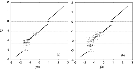
Figure 2: Frequency map for Hamiltonian (23) with $\mu=1$ and with $\varepsilon=0.09$ (a) and $\varepsilon=0.12$ (b). The dotted lines correspond to $\nu=0,-1,-1-\sigma,-1-\sigma^{2}$. $T=1000$.

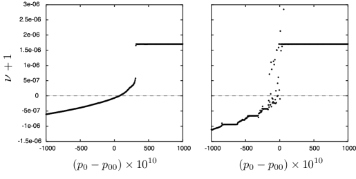
Figure 3: Frequency map for Hamiltonian (23) with $\mu=1$ and with parameter $\varepsilon=0.089$ (a) and $\varepsilon=0.0895$ (b). $\nu+1$ is plotted versus $(p_{0}-p_{00})\times 10^{10}$, where $p_{00}=-3.3307\times 10^{-4}$. The dotted lines corresponds to $\nu=-1$. $T=500000$.

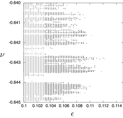
Figure 4: Determination of the last KAM tori for the Hamiltonian (23) with $\mu=1$. For each selected value of the parameter $\varepsilon$, the set of frequencies $\nu$ for which tori are not destroyed is plotted versus $\varepsilon$. The critical value of $\varepsilon$ for which no tori will survive is thus $\varepsilon_{c}\approx 0.11$.

References

- [1] J.M. Greene, A method for determining a stochastic transition, J. Math. Phys. 20 (1979) 1183–1201.
- [2] A. Olvera, C. Simó, An obstruction method for the destruction of invariant curves, Physica 26D (1987) 181–192.
- [3] R.S. MacKay, I.C. Percival, Converse KAM: Theory and practice, Commun. Math. Phys. 98 (1985) 469–512.
- [4] R.S. MacKay, J.D. Meiss, J. Stark, Converse KAM theory for symplectic twist maps, Nonlinearity 2 (1989) 555-570.
- [5] J. Laskar, The chaotic behavior of the solar system: A numerical estimate of the chaotic zones, Icarus 88 (1990) 266–291.
- [6] J. Laskar, C. Froeschlé, A. Celletti, The measure of chaos by numerical analysis of the fundamental frequencies. Application to the standard mapping, Physica D 56 (1992) 253–269.
- [7] J. Laskar, Frequency analysis for multi-dimensional systems. Global dynamics and diffusion, Physica D 67 (1993) 257.
- [8] J. Laskar, Introduction to frequency map analysis, in: C. Simó (Ed.), Hamiltonian Systems with Three or More Degrees of Freedom, NATO ASI Series, Kluwer Academic Publishers, Dordrecht, 1999, pp. 134 – 150.
- [9] M. Govin, C. Chandre, H.R. Jauslin, Kolmogorov-Arnold-Moser–renormalization-group analysis of stability in Hamiltonian flows, Phys. Rev. Lett. 79 (1997) 3881–3884.
-
[10]
C. Chandre, M. Govin, H.R. Jauslin,
Kolmogorov-Arnold-Moser renormalization-group approach to the breakup of invariant tori in Hamiltonian systems, Phys. Rev. E 57 (1998) 1536–1543. - [11] C. Chandre, M. Govin, H.R. Jauslin, H. Koch, Universality for the breakup of invariant tori in Hamiltonian flows, Phys. Rev. E 57 (1998) 6612–6617.
- [12] H. Koch, A renormalization group for Hamiltonians with applications to KAM tori, Erg. Theor. Dyn. Syst. 19 (1999) 475–521.
- [13] J.J. Abad, H. Koch, Renormalization and periodic orbits for hamiltonian flows, Commun. Math. Phys. 212 (2000) 371–394.
- [14] C. Chandre, H.R. Jauslin, A version of Thirring’s approach to the Kolmogorov-Arnold-Moser theorem for quadratic Hamiltonians with degenerate twist, J. Math. Phys. 39 (1998) 5856–5865.
- [15] A. Celletti, L. Chierchia, Construction of analytic KAM surfaces and effective stability bounds, Commun. Math. Phys. 118 (1988) 119–161.
- [16] A. Celletti, A. Giorgilli, U. Locatelli, Improved estimates on the existence of invariant tori for Hamiltonian systems, Nonlinearity 13 (2000) 397–412.
- [17] S. Kim, S. Ostlund, Simultaneous rational approximations in the study of dynamical systems, Phys. Rev. A 34 (1986) 3426–3434.
- [18] W. Thirring, A Course in Mathematical Physics I: Classical Dynamical Systems, Springer-Verlag, Berlin, 1992.
-
[19]
C. Chandre, H.R. Jauslin, G. Benfatto, A. Celletti,
Approximate renormalization-group transformation for Hamiltonian systems with three degrees of freedom, Phys. Rev. E 60 (1999) 5412 – 5421. - [20] B.V. Chirikov, A universal instability of many-dimensional oscillator systems, Phys. Rep. 52 (1979) 263–379.
- [21] C. Chandre, H.R. Jauslin, Strange attractor for the renormalization flow for invariant tori of Hamiltonian systems with two generic frequencies, Phys. Rev. E 61 (2000) 1320 – 1328.