Discrete breathers in dissipative lattices

Abstract

We study the properties of discrete breathers, also known as intrinsic localized modes, in the one-dimensional Frenkel-Kontorova lattice of oscillators subject to damping and external force. The system is studied in the whole range of values of the coupling parameter, from $C=0$ (uncoupled limit) up to values close to the continuum limit (forced and damped sine-Gordon model). As this parameter is varied, the existence of different bifurcations is investigated numerically. Using Floquet spectral analysis, we give a complete characterization of the most relevant bifurcations, and we find (spatial) symmetry-breaking bifurcations which are linked to breather mobility, just as it was found in Hamiltonian systems by other authors. In this way moving breathers are shown to exist even at remarkably high levels of discreteness. We study mobile breathers and characterize them in terms of the phonon radiation they emit, which explains successfully the way in which they interact. For instance, it is possible to form “bound states” of moving breathers, through the interaction of their phonon tails. Over all, both stationary and moving breathers are found to be generic localized states over large values of $C$, and they are shown to be robust against low temperature fluctuations.

I INTRODUCTION

The phenomenon of (non-topological) localization in discrete nonlinear lattices (i.e. intrinsic localized modes or discrete breathers) has received a great deal of attention from both theoretical and (as of lately) experimental research. Indeed, recent observations [1, 2, 3] of discrete roto-breathers in Josephson-junction ladder circuits have placed the subject on a firm experimental footing (see also [4]). Most of the theoretical and computational work on discrete breathers has dealt with Hamiltonian systems, of fundamental interest in Physics. For a review, see Refs. [5, 6]. Comparatively, the easier case of dissipative breathers has received much less attention, though the experimental systems that we have just mentioned belong to this class.

Mathematical proofs of existence of discrete breathers in rather general dissipative networks of oscillators [7, 6] appeared soon after those of Hamiltonian networks [8]. While in the later case, a condition of non-resonance of the localized oscillation with the band of extended normal modes of the lattice has to be satisfied, that is not an issue in the forced-damped case, and the dissipative breather possesses the character of attractor for initial conditions in the corresponding basin of attraction. As archetypical example of Klein-Gordon lattices of oscillators, we consider the standard Frenkel-Kontorova model with commensurability one (i.e. average interparticle distance equal to the period of the sinusoidal substrate potential). In section II we discuss the numerical procedures used to obtain accurate breather solutions, which are based on the continuation from the uncoupled limit of the model.

In section III we explain some general features of the linear stability (Floquet) analysis of forced-damped periodic discrete breathers. For the sake of readability, this section is intended to be self-contained, to some extent. After deriving some straightforward properties of the Floquet multipliers, we obtain some formal conditions for the non-appearance of extended instabilities of the uniformly oscillating background, along with the tail analysis valid for not-too-large forcing. The good fitting of our numerical data to the results of this section ensures its validity for the parameters used in the numerical work.

Section IV reports on our numerical findings, concerning pinned discrete breathers, which are summarized in the phase diagram against the coupling parameter. Pitchfork and Andronov-Hopf bifurcations separating different periodic and quasiperiodic breathers appear as generic features of this phase diagram. At very high values of the coupling parameter, when the width of the discrete breather is much larger than the period of the substrate potential, a Goldstone mode in the Floquet spectrum signals the approach to the continuum limit.

In section V we study the mobility of discrete breathers, a subject which is yet poorly understood. After discussing the procedures used to obtain and continue mobile breathers we explain successfully, with the aid of simple physical arguments, the numerical power spectra in the tails. Then we study collisions between discrete breathers. We find all possible scenarios, ranging from “elastic” to completely “inelastic” collisions; this latter case includes both breather annihilation and, more interestingly, the formation of “breather molecules” which can be either pinned or mobile. Finally, in section VI, we summarize the main conclusions of our work.

II MODEL AND BREATHER GENERATION

The equations of motion of the Frenkel-Kontorova chain subject to damping and an (spatially uniform) external driving force are, in dimensionless form,

$$\ddot{u}_{j}+\alpha\dot{u}_{j}+ \frac{1}{2\pi}\sin(2\pi u_{j})=$$ (2)

$$C\left(u_{j+1}-2u_{j}+u_{j-1}\right)+F_{ac}\sin(\omega_{b}t)$$

In order to generate a discrete breather configuration we start in the anti-integrable (uncoupled) limit $C=0$, using two different amplitude attractors of the single pendulum equation of motion. That is, we first consider the dynamics of a single forced and damped pendulum, and try to find a region of parameters where there is at least two different attractors coexisting. Note that, generically, all oscillators have at least two attractors for sufficiently low values of the damping $\alpha$ and the force $F_{ac}$, if the frequency of the force $\omega_{b}$ is not wildly different from the typical frequencies of the autonomous oscillator.

Therefore we initially choose values for $\alpha$, $F_{ac}$, and $\omega_{b}$, and keep them fixed while we vary $C$. Then, for instance, we fix one of the oscillators to the high amplitude solution and all the others to the low one. Using as initial condition this anti-integrable configuration, we turn on adiabatically the coupling parameter $C$. Following Sepulchre and MacKay’s work on dissipative breathers [7], the initial solution can be continued for $C\neq 0$, at least until a bifurcation is reached. That paper shows how, in contrast to Hamiltonian systems, forced and damped systems have it easier to comply with the conditions of the continuation theorem, since there is no problem of resonance with phonons (we have attractors), and the relative phases of the oscillators are locked by the external force.

Moreover, if the variation in $C$ is small enough, the discrete breather remains an attractor of the dynamics (since one expects the basins of attraction to evolve continuously with $C$ as well). This makes the numerical continuation greatly simpler: it is possible to just vary adiabatically the coupling $C$ as we integrate the equations of motion (2), and the dissipative dynamics drives the system to the stable attractor. Contrast this with the expensive root-finding methods one needs to use for breather continuation in Hamiltonian problems [9].

In addition, we performed a linear stability analysis of the periodic solutions (Floquet-Bloch analysis, see below) in order to investigate the nature of possible bifurcations. In some cases we have added to the initial conditions a small random noise (typically of order $10^{-5}$) to test for robustness. We have taken special care dealing with finite size effects. For low values of $C$ ($C<0.6$) small lattice sizes can be used (say $N=40$). However, once the breather is dressed by a phonon tail (see below), we have needed to increase the lattice size up to $N=900$ in order to avoid finite size effects. We think this is an important point to check since experiments in real dissipative systems are done in small lattices [1, 2]. Numerical integration of equations of motion has been done using a fourth-order Runge-Kutta scheme. Most of the simulations in this paper have been done with the following parameters: $\alpha=0.02$, $\omega_{b}=0.2\pi$, and $F_{ac}=0.02$, although we have sometimes changed them to confirm the general validity of our results.

III LINEAR STABILITY ANALYSIS

A Floquet multipliers

Let us consider a small perturbation, $\{v_{j}(t)\}$, of the discrete breather $\{u_{j}(t)\}$ solution, $v_{j}=u_{j}+\epsilon_{j}$. After direct substitution in the equations of motion and discarding terms which are nonlinear in $\epsilon_{j}$, one finds

$$\ddot{\epsilon}_{j}+\alpha\dot{\epsilon}_{j}+\cos(2\pi u_{j}(t))\epsilon_{j}=C\left(\epsilon_{j+1}-2\epsilon_{j}+\epsilon_{j-1}\right)$$ (3)

These form a system of coupled linear differential equations with time periodic coefficients, for $u_{j}(t)$ is a periodic function of time. For a system of size $N$, the integration of the linearized equations (3) over a period $t_{b}=2\pi/\omega_{b}$ of each of the $2N$ vectors $\{\epsilon_{j}(0),\dot{\epsilon}_{j}(0)\}$ forming some basis of the tangent space defines the $2N\times 2N$ Floquet (or monodromy) matrix $\cal F$

$$\left(\begin{array}[]{c}\epsilon_{j}(t_{b})\\ \dot{\epsilon}_{j}(t_{b})\end{array}\right)=\cal{F}\left(\begin{array}[]{c}\epsilon_{j}(0)\\ \dot{\epsilon}_{j}(0)\end{array}\right)$$ (4)

that relates the small perturbations at $t=t_{b}$ to those at $t=0$; in other words, $\cal F$ is the matrix associated to the $t_{b}$-map of (3).

The linear stability of the breather solution $\{u_{j}(t)\}$ requires that all the eigenvalues of the Floquet matrix (called also Floquet multipliers) are inside the unit circle. Since $\cal F$ is real, if $\mu$ is an eigenvalue of $\cal F$, its complex conjugate $\overline{\mu}$ is also an eigenvalue of $\cal F$. But the Floquet spectrum has more structure, since one can transform the linear system of Eq. (3) into a Hamiltonian one (see Ref. [10]). By transforming the $\epsilon_{j}$ variables according to

$$\epsilon_{j}(t)=e^{-\alpha t/2}\eta_{j}(t),$$ (5)

this yields

$$\ddot{\eta}_{j}-\Bigl{(}\alpha^{2}/4-\cos\bigl{(}2\pi u_{j}(t) \bigr{)}\Bigr{)}\eta_{j}=$$ (7)

$$C(\eta_{j+1}-2\eta_{j}+\eta_{j-1})$$

These are the equations of motion of a (non autonomous) Hamiltonian system of oscillators, for which the eigenvalues of the (symplectic) $t_{b}$-map must come in pairs such that their product is unity. Together with the fact that the map is real, one has these well known [11] three possible cases: (i) pairs of eigenvalues lying on the unit circle, with $\lambda_{1}=\overline{\lambda}_{2}$; (ii) pairs lying on the real axis, with $\lambda_{1}=1/\lambda_{2}$; (iii) 4-tuples of eigenvalues with $\lambda_{1}=\overline{\lambda}_{3}$, $\lambda_{2}=\overline{\lambda}_{4}$, $\lambda_{1}=1/\overline{\lambda}_{4}$.

Since the transformation (5) scales the eigenvalues by a factor $\exp[-\alpha t_{b}/2]$, the Floquet multipliers of (3) must either lie on a circle of radius $\exp(-\alpha t_{b}/2)$, or on the real axis such that $\mu_{1}\mu_{2}=\exp(-\alpha t_{b})$, or come as 4-tuples such that $\mu_{1}=\overline{\mu}_{3}$, $\mu_{2}=\overline{\mu}_{4}$, $\mu_{1}=\exp(-\alpha t_{b})/\overline{\mu}_{4}$.

An important difference with the Hamiltonian case, where a “phase” and the “growth” modes [6] are always associated to the double eigenvalue $+1$ in the Floquet matrix of the discrete breather, is that these modes do not exist for the forced-damped case. The reason for that is that both the breather frequency and the time origin are fixed by the external force, so that the associated degeneracies are removed.

B Extended instabilities

In the limit of an infinite system ($N\rightarrow\infty$), the spectrum of $\cal F$ consists of a continuous part associated with spatially extended eigenvectors and a discrete part associated with spatially localized eigenvectors. The continuous part of the spectrum of $\cal F$ is the continuous spectrum of the linearized problem around the homogeneous solution (i.e., without breather) $\{u_{j}(t)\}=\{u_{\infty}(t)\}$. As pointed out by Marín and Aubry [12], using the fact that the limit (in the appropriate sense) of the sequence of spatial translations of the Floquet matrix $\cal F$ of the system with breather is the Floquet matrix ${\cal F}_{0}$ of the system without the breather, one proves easily that the spectrum of ${\cal F}_{0}$ is included in the spectrum of $\cal F$. Reciprocally, the limit of the sequence of spatial translations of an extended eigenvector of $\cal F$ can be seen to belong to the spectrum of ${\cal F}_{0}$.

First, we are going to consider the spectrum of ${\cal F}_{0}$, so we now will pay attention to the linearized equation of motion (3) around the homogeneous solution of (2), $\{u_{j}(t)\}=\{u_{\infty}(t)\}$ and denote simply $f(t)=\cos(2\pi u_{\infty}(t))$. Under the usual periodic boundary conditions, we look for solutions of the linear problem with the plane-wave form

$$\eta_{j}(t)=e^{iqj}\chi^{q}(t)$$ (8)

In other words, $\chi^{q}(t)$ is the (spatial) Fourier coefficient of $\eta_{j}(t)$. Inserting (8) into the equations (3), and denoting by $E(q)=4C\sin^{2}(q/2)-\alpha^{2}/4$, we have, for each value of $q$, the equation

$$\ddot{\chi}^{q}(t)+\bigl{(}E(q)+f(t)\bigr{)}\chi^{q}(t)=0$$ (9)

This is a Hill equation. For each solution $\chi^{q}(t)$ of the single Hill equation (9) we have a solution of the form (8) for the equations (7), and thus, a solution

$$\epsilon_{j}(t)=e^{iqj}e^{-\alpha t/2}\chi^{q}(t)$$ (10)

for the linearized problem. The Hill equation (9) has a general solution which can be expressed in terms of its normal solutions, which have the property

$$\chi^{q}(t+2\pi/\omega_{b})=\lambda_{q}\chi^{q}(t),$$ (11)

where $\lambda_{q}$ is called the characteristic number of the equation. The complex number $\rho_{q}$ defined as $\lambda_{q}=\exp(2\pi\rho_{q}/\omega_{b})$ is the called characteristic exponent (its imaginary part being defined up to an additive multiple of $\omega_{b}$). In the generic case in which equation (9) has two different characteristic numbers $\lambda_{q}^{+},\lambda_{q}^{-}$, their product is equal to unity, $\lambda_{q}^{+}\lambda_{q}^{-}=1$, and the general solution has the form

$$\chi^{q}(t)=c_{+}e^{\rho_{q}^{+}t}\psi_{q}^{+}(t)+c_{-}e^{\rho_{q}^{-}t}\psi_{q}^{-}(t)$$ (12)

where $c_{+},c_{-}$ are constants and $\psi_{q}^{+},\psi_{q}^{-}$ are time periodic functions with period $2\pi/\omega_{b}$. Consequently, $\chi^{q}(t)$ is bounded by $K\exp(\rho^{\text{max}}_{q}t)$, with $K$ some constant, and $\rho^{\text{max}}_{q}=\max\{\rho_{q}^{+},\rho_{q}^{-}\}$. Thus, from equation (10), we conclude that the stability of the homogeneous solution $\{u_{\infty}(t)\}$ is assured in the parameter region in which

$$\rho_{\text{sup}}=\sup_{q}\rho_{q}^{\text{max}}<\alpha/2$$ (13)

The determination of this region in parameter space can only be made by numerical means. For the range of parameters that we have used in our study of damped-forced breathers, the function $f(t)$ is a low amplitude oscillation around the value $1$, and, as expected from the well-known results on weakly time dependent Hill equations, we have not observed instabilities by extended modes.

In the next section, we will follow the continuation of the breather solution from the uncoupled limit, for increasing coupling and numerically compute the eigenvalues of the Floquet matrix ${\cal F}$. This will allow the characterization of the different bifurcations that the breather experiences when the coupling parameter increases.

C Tail analysis

To proceed a bit further, we will assume from now on in this section that $u_{\infty}(t)$ is an oscillation of very low amplitude, so that for $|j|\gg 1$ the coefficient $\cos(2\pi u_{j}(t))$ in equations (3) is essentially unity, if one discards terms less than or equal to $u^{2}_{\infty}(t)$. Then we are left with the standard problem of a linear chain with damping, which we can solve exactly (a similar analysis to the one below appears in Ref. [13]).

Let us consider a semi-infinite chain with the boundary condition at the beginning given by $\epsilon_{0}(t)=\exp(-i\omega t)$, and look for solutions of (3) of the form

$$\epsilon_{j}(t)=e^{(-\xi+iq)j}e^{-i\omega t}$$ (14)

Inserting (14) into equations (3) one obtains for the real and imaginary part, respectively

$$\cosh\xi\cos q = 1+\frac{1}{2C}(1-\omega^{2})$$ (16)

$$\sinh\xi\sin q = \frac{\alpha\omega}{2C}$$ (17)

First, we will analyze the situation in which $\alpha=0$, and see how one recovers the well-known results for Hamiltonian discrete breathers [14, 15]. For $\xi=0$, one has the familiar normal mode solutions, where the frequencies are given by the dispersion relation

$$\omega^{2}=1+4C\sin^{2}(q/2)$$ (18)

and $q$ ($-\pi<q<\pi$) is the wave-vector of the normal mode. It is customary to denote loosely the normal modes as “phonons”, and the interval of values of $\omega$ defined by (18) as “phonon band”. For $\xi\neq 0$ one has exponentially decaying solutions

$$\epsilon_{j}(t) = e^{-\xi j}e^{-i\omega t}$$ (20)

$$\epsilon_{j}(t) = (-1)^{j}e^{-\xi j}e^{-i\omega t}$$ (21)

where the inverse decay length $\xi$ and the frequency $\omega$ are related, respectively, through:

$$\omega^{2} = 1-4C\sinh^{2}(\xi/2)$$ (23)

$$\omega^{2} = 1+4C\cosh^{2}(\xi/2)$$ (24)

Note that the values of $\omega$ in (III C) are, respectively, below and above the phonon band, so we observe how the Hamiltonian linear lattice damps out any solution with a frequency component outside the phonon band (18), while the normal modes are extended ($\xi=0$). As a consequence, a Hamiltonian breather needs to have all breather harmonics $n\omega_{b}$ out of the phonon band, and then they decay exponentially with the characteristic length $\xi^{-1}(n\omega_{b})$. Thus the size of the Hamiltonian breather is given by $\xi^{-1}_{b}=\sup_{n}\xi^{-1}(n\omega_{b})$.

When $\alpha\neq 0$, we have that $\xi(\omega)\neq 0$. Thus, any solution decays exponentially. For very low values of the damping, and frequencies well inside the (Hamiltonian) phonon band, the decay length $\xi^{-1}$ is very large, so that $\sinh\xi\simeq\xi$ in equation (17), and thus it can be approximated by

$$\xi^{-1}\simeq\frac{2C\sin q}{\alpha\omega}=\frac{2v_{g}}{\alpha}$$ (25)

where $v_{g}=(d\omega/dq)$ is the “group velocity” of the corresponding normal mode, obtained from the dispersion relation (18). This approximation admits a simple physical interpretation in terms of the competition between the damping and the velocity $v_{g}$ at which the wave generated (at the beginning of the semi-infinite chain) by the sustained perturbation propagates: The amplitude of the excited phonon decays in time as $\exp(-\alpha t/2)$, so that the time after which the amplitude has decayed by a factor of ($1/e$) is $2/\alpha$, and thus the distance traveled by the phonon is $2v_{g}/\alpha$.

An example of the solutions $\xi(\omega)$ and $q(\omega)$ of equations (III C), for the particular values $\alpha=0.02$ and $C=0.75$, appears in Fig. 1. For comparison purposes, the graphs corresponding to the same value of coupling for the Hamiltonian case are included.

Note that for the existence of damped-forced discrete breathers there is no need of a non-resonance condition (in contrast with the Hamiltonian case), because for any frequency $\omega$, $\xi(\omega)\neq 0$. However, for low values of $\alpha$, if some breather harmonic $n\omega_{b}$ belong to the interval of values of $\omega$ for which $\xi(\omega)$ is very small, the breather profile will show large “wings”. In Fig. 2 we plot $\xi(3\omega_{b})$ as a function of the coupling $C$, for $\alpha=0.02$ and $\omega_{b}=0.2\pi$. Observe the dramatic decay of $\xi(3\omega_{b})$ at around $C=0.6$ corresponding to the entrance of the third breather harmonic in the (so to speak) “phonon band”, and compare the breather profiles for two values of C, respectively below and above, in Fig. 3. Both the wave-vector and the size of the wings in figure fit very well with $q(3\omega_{b})$ and $\xi(3\omega_{b})$ from equations (III C).

IV BIFURCATIONS AND PHASE DIAGRAM

We have continued numerically breather solutions from the uncoupled (or anti-integrable) limit, for fixed values of the damping coefficient ($\alpha=0.02$), external force frequency ($\omega_{b}=0.2\pi$) and intensity ($F_{ac}=0.02$). The spectrum of Floquet multipliers was also numerically computed for each solution, thus monitoring their evolution on the complex plane. The configurations we have focused on are two: the one-site breather and the two-site breather (adjacent sites). Of course many other configurations are possible, by choosing from all combinations of sites in either the high-amplitude or low-amplitude attractor. However these two simplest breathers already provide a quite rich behavior, and, surprisingly, they allow continuation into very high values of $C$, where the continuum limit is approached.

At very low values of $C$ the continued one-site breather is very narrow, symmetric around its localization site (i.e. $u_{-i}(t)=u_{i}(t)$ for all $t$ and $i$), and all the Floquet multipliers lie on the circle of radius $\exp(-\alpha t_{b}/2)$ in the complex plane. The breather remains stable for increasing coupling up to the value $C_{\text{P1}}=0.52962$ where a Floquet multiplier, which had previously detached along the real axis from that inner circle, reaches the unit circle at $+1$. The corresponding eigenvector of the Floquet matrix is localized around the breather site and possesses odd mirror symmetry with respect to that site, as shown in Fig. 4. Past the bifurcation, we are left with an unstable symmetric breather and two new stable breathers, spatially asymmetric and one being the mirror image of the other. We can conclude that this is a forward pitchfork bifurcation [16], associated to a spatial symmetry-breaking transition of the discrete breather.

In order to visualize the mirror symmetry breaking character of this bifurcation, we plot in Fig. 5 the difference $\Delta(0)=u_{-1}(0)-u_{1}(0)$ at time $t=0\pmod{t_{b}}$ of the positions of the neighbor oscillators on both sides of the localization site, as a function of the coupling parameter $C$ in the vicinity of the bifurcation value. It is not surprising that, close to the bifurcation, the difference $\Delta(0)$ scales with the coupling parameter as $(C-C_{\text{P1}})^{1/2}$, because the one-dimensional character of the unstable manifold of the symmetric breather allows to reduce the analysis to that of a pitchfork bifurcation in a one-dimensional map, where this scaling behavior for the distance between branches is well-known.

The asymmetric stable branches born at $C_{\text{P1}}$ can be continued for higher values of coupling. We then observe how the amplitude of one of the neighbors of the central site keeps increasing, until it equals the amplitude of the central oscillator (which has in turn decreased slightly), at $C_{\text{P2}}=0.55315$. It should be noted that the relative phases of the oscillators do not appear to change, At this value, a backward pitchfork bifurcation occurs, where the two stable asymmetric breathers and one unstable symmetric two-site breather merge, and a stable mirror-symmetric two-site breather comes out. As in the bifurcation analyzed before, only one Floquet eigenvector, associated to a Floquet multiplier of value $+1$, is involved.

This unstable two-site breather which joins this second pitchfork is nothing but the two-site breather which can be continued from the uncoupled limit. Thus we have that the two elementary breathers constructed at the uncoupled limit, one-site and two-site, undergo an exchange of stability via this symmetry-breaking pitchfork mechanism. For $C<C_{\text{P1}}$ the one-site breather is stable and the two-site one unstable. For $C_{\text{P1}}<C<C_{\text{P2}}$ both are unstable, and the new asymmetric breather is stable. Past $C_{\text{P2}}$, the two-site breather is stable and the one-site unstable. This is exactly the same mechanism that was previously found by other authors [17] for Hamiltonian breathers, and which is related to breather mobility as we explore in the next section. It is therefore plausible to conjecture that the mechanism is highly generic and might be expected in a large class of models.

To be thorough in our description, a much less interesting bifurcation does appear in the two-site breather branch at very low $C$. The two-site breather is initially stable at the uncoupled limit, but loses stability after a pitchfork bifurcation at $C\approx 0.02$. This is also a symmetry-breaking bifurcation as above, however it is instructive to investigate the differences: this time the spatial symmetry is broken in such a way that the new stable, asymmetric breathers suffer a de-phasing between the two central sites. This can be confirmed rigorously by examination of the relevant eigenvector at the bifurcation. If one takes as reference for the time origin the instant at which the two central sites have maximum amplitude, the unstable eigenvector for this second pitchfork shows components only in the velocity part, not in amplitudes; the former bifurcation shows exactly the opposite behavior. In any case, the continuation of the asymmetric breather from this bifurcation at $C=0.02$ is quickly lost after a Hopf bifurcation, and we have not found any more interesting behavior arising from these curious branches.

Now we turn on to the continuation of the stable two-site breather branch past $C>C_{\text{P2}}$. We find now that near $C=0.817$ two complex conjugate Floquet multipliers cross the unit circle at $\exp(\pm i\varphi)$, with $\varphi=1.285$, and the (periodic) two-site breather becomes unstable. The real and imaginary components of the associated eigenvectors are shown in Fig. 6. Close to the bifurcation, small perturbations of the unstable periodic breather bring it into a quasiperiodic breather (as verified by inspection of the Poincaré section), thus confirming the scenario of an (Andronov-) Hopf bifurcation [18]. Indeed, the power spectrum analysis of the quasiperiodic attractor (see figure) reveals two basic frequencies, $\omega_{b}$ and $\omega_{\text{new}}=0.0873$. However, since this new frequency is rather different from the frequency $\varphi\omega_{b}/2\pi=0.1285$ associated to the destabilizing eigenvalue couple, one concludes that the stable quasiperiodic attractor does not come out straight from the bifurcation. In other words, the simplest scenario of a subcritical Hopf bifurcation is discarded. Moreover, the quasiperiodic attractor can be easily continued back for lower values of the coupling (i.e., $C<0.817$), therefore confirming that we have a subcritical Hopf bifurcation. Note that, as parameters other than $C$ change, it is possible for these subcritical Hopf bifurcations to become supercritical, for their genericity lies in the Hopf character, not in being subcritical or supercritical.

The lack of periodicity for the new (quasiperiodic) breather attractor prevents the use of Floquet analysis. However, its stable character can be numerically ascertained, checking its robustness against small perturbations in the dynamics. This quasiperiodic two-site breather turns out to be stable for couplings up to $C=0.88$, beyond which it starts moving spontaneously. Only when we reach $C=0.96$ we recover again a stable, pinned quasiperiodic breather. Meanwhile, the pinned, periodic two-site breather (which became unstable after the Hopf bifurcation at $C=0.817$) can be continued by a Newton method. At a value near $C\approx 0.995$, it rejoins the quasiperiodic two-site breather in an inverse (now supercritical) Hopf bifurcation, becoming stable again.

We have tried to summarize most of these bifurcations in the sketch of Fig. 8. We postpone to the next section the analysis of the observed mobile breathers in this region (and others) of parameter space.

To conclude this section we will comment on the continuation and stability analysis as $C\rightarrow\infty$, i.e. the so-called continuum limit. The first interesting fact is that both the one-site and two-site breather, whether stable or unstable, have been found to be continuable for couplings as high as desired. In other words, they never disappear by, say, saddle-node bifurcations or the like. Another interesting point is that for $C>1$ we have also found pitchforks which connect the two branches, exactly in the same way as the first one at $C_{\text{P1}}$, $C_{\text{P2}}$. The ranges of coupling between forward and backward pitchfork bifurcations (that is, where the connecting branches of stable asymmetric breathers exist) get progressively narrower for higher coupling values. And finally, both the breather profiles and their Floquet spectrum reveal a very natural approach to the continuum limit: the solutions get broader in size, while the eigenvalue responsible for the pitchforks remains closer and closer to $+1$ at all times, announcing the appearance of the Goldstone mode (due to translational invariance) as $C\rightarrow\infty$. These effects were ostensibly manifest at $C\gtrsim 5$.

V MOBILE BREATHERS

The problem of the mobility of discrete breathers is still very poorly understood. While the fundamental theory of stationary breathers is now firmly established [8], moving discrete breathers (MB for short) have so far eluded a rigorous treatment. But the fact is that moving breathers have been observed and studied through numerical simulation in various works [19, 20, 21, 17, 22], and they appear to be a phenomenon with the same degree of genericity as the stationary case. Up to now most of those works have dealt with Hamiltonian systems; here we present a study of moving breathers in our forced and damped F-K model. Some of the results are strikingly similar to those observed in Hamiltonian systems.

We should first point out that a moving breather is something to be distinguished from a similar class of solutions, namely lattice solitons [23, 24]. In a lattice soliton a pulse propagates without dispersion through the lattice, but, unlike breathers, there is no “internal” oscillation. This additional degree of freedom makes the moving breather a more complicated object. For instance, in Hamiltonian lattices, it is easy to see that inevitably the moving breather resonates with the phonon band (note the presence of a quasi-periodic spectrum due to the additional frequency introduced by the translational motion), and therefore it is not possible to have tails which decay to zero. It is not clear whether the solution is just a transient which eventually decays by phonon radiation, or maybe an infinite lifetime breather which “rides” on an infinite, small amplitude radiation background.

But our model here is dissipative and has external forcing, and it turns out that moving breathers appear as proper attractors of the dynamics. Since these solutions are not transients, we can study and characterize them accurately and with great confidence. Even though this will not shed any light on the problem of existence of Hamiltonian moving breathers, there is another aspect of theoretical interest in which this study can contribute: the (possible) concept of a Peierls-Nabarro barrier for breather motion. This concept arises because of the similarities with the problem of mobility of discommensurations (kinks) in the Frenkel-Kontorova model [25]. The discommensuration is an equilibrium static structure, for which one may ask how much energy it costs to displace it by one lattice site, until it reaches the equivalent configuration by (discrete) translational invariance. This is commonly referred to as the Peierls-Nabarro (PN) barrier. And it is possible to give a precise definition: from all possible continuous deformations of the initial configuration into the final one, take the one in which the maximal energy change along the path is the minimum. Very fruitful results in the theory of the F-K model have stemmed from this definition [25].

But a corresponding definition of a PN barrier for breathers proves quite problematic. The difficulty lies in that it is not clear which space to use, since the configurations are now periodic functions, not static points. Some authors have suggested possible candidates for a rigorous definition, but the issue is still under debate [26, 6, 27]. Technicalities aside, it is still possible to give a working definition of the Peierls-Nabarro barrier for breathers, at least in some cases. Most studies generate moving breathers by perturbing stationary ones, and Ref. [28] gave a systematic method to do this. Looking at the linear stability analysis of the breather (Floquet analysis), they found that in many cases one can identify an eigenmode which is distinctively localized and whose spatial symmetry is the appropriate for breather motion (note that similar depinning modes are responsible for the depinning of discommensurations [25] under uniform forcing). It was found that adding a perturbation along this depinning eigenmode, provided one overcomes a certain threshold, results in a moving breather. Such thresholds are probably the best pragmatic approach to the definition of a PN barrier.

A further study [17] showed that many Hamiltonian lattices exhibit a very interesting behavior which is linked to mobility. It was found that, as the coupling is increased from $C=0$, the one-site breather and the two-site breather each undergo a pitchfork bifurcation, where new branches of periodic but spatially asymmetric breathers emerge. These branches do in fact connect those pitchfork points, and the corresponding Floquet eigenmodes responsible for the bifurcations obviously show a spatial symmetry which we could dub as “depinning”. This is exactly what we have found in our dissipative model, as shown in the previous section. And, just as in the cited works on Hamiltonian systems, we have also verified that the mobility is greatly enhanced for values of coupling in the vicinity of these bifurcations: very small amounts of perturbation along the depinning mode are enough to create the mobile breather. The upshot is that this phenomenon provides a mechanism for the existence of mobile breathers at relatively low couplings (high discreteness) and with very slow velocities, two properties which were counterintuitive and unexpected.

We should note that the continuous sine-Gordon equation under external ac forcing and losses does not support MB solutions [29]. The way in which a continuous breather destabilizes is by a transition to a quasiperiodic state and finally creation of a kink-antikink pair [30].

In the following we begin exploring this relation between the stability of stationary breathers and the existence of their mobile counterparts. Then we concentrate on studying the properties of moving breathers in dissipative systems in more detail. Finally, we explore other aspects such as collisions.

A Generation and phase diagram of MB

We have found MB as proper attractors of the dynamics in a wide range of couplings, in particular for $0.5\lesssim C\lesssim 0.96$. We have found them either by excitation of the depinning mode of stationary breathers (as explained below) or simply by letting the system evolve to a steady state after the instabilities of some stationary breathers develop fully. Then it is possible to carry out a continuation of the MB into other parameter values, since their attractor property allows to change slowly a parameter and track the MB solution. Figure 9 shows the phase diagram of MB we have constructed with this procedure.

Around the first symmetry-breaking bifurcation there is a narrow region in which we found MBs with regular motion and well defined velocity (Fig. 10). A similar region is found in the interval $0.7\lesssim C\lesssim 0.88$. We call these solutions induced fast breathers. To generate these steady state MB we have followed the procedure described in [28]. Surprisingly, this method works very well not only near the bifurcations. We typically use as initial conditions:

$$u_{i}(t=0)=u^{0}_{i}+\lambda\epsilon^{a}_{i},$$ (26)

where $u_{i}^{0}$ is a stationary breather solution, $\epsilon^{a}_{i}$ corresponds to the antisymmetric (and localized) eigenvector mode at the bifurcation taking place near $C=0.53$, and finally $\lambda$ measures the strength of the perturbation applied. It is found that, as in the Hamiltonian case, a critical $\lambda_{c}$ is necessary to unpin the breather. However, in contrast to the results for Hamiltonian systems, once the breather starts to move the velocity is unique (independent of $\lambda$), i.e. the MB is a robust attractor of the dynamics. Once a induced MB is generated at a value of $C$, this solution can be continued by varying $C$ slowly, with almost no variation in velocity. The analysis of Poincaré sections of this MB shows clearly a quasiperiodic behavior. Therefore there is not commensurability between the internal frequency $\omega_{b}$ and the new frequency associated to the velocity $\omega_{\text{mb}}=2\pi v_{\text{mb}}$. This behavior precludes the use of fixed point methods (like Newton method) based in the periodicity of solutions, to find (numerically) exact MB solutions. Also, this quasiperiodicity prevent us to extend the Floquet analysis to MB.

For intermediate couplings $0.60\lesssim C\lesssim 0.72$ (shadow region in the phase diagram), the breather portrays random motion. For some time interval, the MB moves regularly in one direction, then suddenly remains inmobile (but quasiperiodic) for a while, changing then its motion to the other direction, and so on. A plausible scenario is that of the occurrence of a crisis [31] at $C\approx 0.72$ which destabilizes the regularly moving breathers (of positive and negative velocity, respectively), giving rise to a chaotic attractor consisting of intervals (of random length) of approximately regular motion, followed by changes of direction.

As we have already mentioned, at $C=0.88$ the stationary breather solution (quasiperiodic) disappears, and only the MB solutions survive. We will refer to this breather as spontaneous slow MB. Its velocity is approximately half of the fast MB and shows a great variation as a function of $C$. Moreover, there is a narrow window around $C=0.89$ where both the slow and fast MB coexist.

Regular motion MB are also stable against variation of parameters other than $C$. By increasing $F_{ac}$, the velocity of the breather increases, showing a very asymmetric profile, as shown in Fig. 11. As we explain below, the origin of this asymmetric shape can be explained in terms of forward and backward emission of phonons from the moving breather, which suffer a Doppler effect. Above a critical value of $F_{ac}$, which is dependent on $C$, a shock wave is formed and the regular motion becomes again diffusive.

B Emission of phonons

An important feature of both pinned quasiperiodic and moving breathers is the emission of low amplitude linear waves (phonons). In both cases the breather tails clearly show a complex quasiperiodic behavior in which many frequencies are involved. For the moving breather, these tails are also markedly asymmetric, due to the translational motion. Other authors have investigated the behavior of Hamiltonian breathers when subject to phonon scattering [15]; note that in our case it is the breather itself the source of phonons.

In order to investigate the phonon emission we have computed the power spectrum of $\dot{u}_{i}(t)$ for sites sufficiently far away from the breather center, as given by the expression

$$S(\omega)=\left|\int_{-\infty}^{\infty}\dot{u}_{j}(t)e^{i\omega t}dt\right|^{2}$$ (27)

In all spectra, we can observe peaks corresponding to the driving frequency and its odd harmonics, as expected. We also observe a broad band spectrum corresponding to frequencies in the phonon band, with several resonant peaks. In both cases we can explain those frequencies satisfactorily in terms of emission of phonons by the breather.

Figure 12 shows a time snapshot and the corresponding power spectra for a particle in the tails of a quasiperiodic pinned breather. In this case, the resonant peaks simply correspond to frequencies which are linear combinations of $\omega_{b}$ and $\omega_{\text{new}}$ (the second basic frequency of the quasiperiodic breather):

$$\omega_{\text{tail}}=m\omega_{b}+n\omega_{\text{new}},\qquad m,n\in{\mathbb{Z}}$$ (28)

In the case of moving breathers, the peaks also correspond to the frequencies given above, but shifted by the Doppler effect since they are emitted by a moving source. Their calculation requires thus a little more care. We recall that the propagation of phonons is given by the dispersion relations (III C). The frequency of the emitting source, in the reference frame of the source itself, is $\omega_{\text{src}}=n\omega_{b}+2\pi mv_{\text{mb}}$. This second frequency appears because the breather is moving over a periodic potential with velocity $v_{\text{mb}}$. However, in the reference frame of the medium (the lattice), this frequency will be modified according to:

$$\omega_{\text{tail}}=\omega_{\text{src}}\pm 2\pi q(\omega_{\text{tail}})v_{\text{mb}},$$ (29)

which is the well-known Doppler effect, only that the medium is dispersive [32]. In particular, note how the wavevector $q$ of the propagated phonon depends on $\omega$, as given by Eqs. (III C). Therefore Eqs. (III C) and (29) have to be solved self-consistently for $q$ and $\omega_{\text{tail}}$, and then the different peaks of the power spectrum can be worked out. The agreement of this calculation with the observed frequencies (see Fig. 13) is excellent.

Finally we remark that for small lattice sizes, and when using periodic boundary conditions, tails in front of and behind the breather can overlap. In such cases, solutions are similar to the so-called nanopterons [33] of Hamiltonian systems, in which the MB appears to move in a “sea” of phonons.

C Breather Collisions and Thermal Effects

Since we are dealing with a system in which pinned (periodic and quasiperiodic) and mobile breathers coexist for the same parameter values, it seems natural to study their stability against collisions between them. Very different kind of events appear depending on the breather velocity and the initial conditions (initial distance between breathers). The faster the breathers are, the more likely they are to destroy each other. The main result is that, when the breathers survive to the collision, the interaction is mediated by the phonons which dress the breather. For large velocity, the tail in front of the breather is short (the MB is very asymmetric), so the breather cores can overlap and we observe they get destroyed. For moderate velocities, the opposite occurs: the tails are large, and it seems as if they mediated the collision, slowing down the breathers and preventing the cores to touch. A clear example of this latter case can be seen in the figure 14, where we observe an “elastic” collision in which the breathers approach each other up to a distance which is the range of the phonon tail. Note that this distance ($\approx 150$) is much larger than the core breather size ($\approx 10$).

In figure 15 we show some of the multiple behaviors we have observed in simulations: (i) Collision between two MB at low $F_{ac}$ and thus low velocity, at $C=0.75$. Their velocity is low enough to not destroy themselves, but to create a new multibreather state; (ii) elastic collision of two “slow” breathers at $C=0.89$; (iii) collision which gives a mobile two-breather state. The last two collisions only differ in the initial conditions. Finally, (iv) breather annihilation between a “slow” and “fast” breather at $C=0.89$ where they coexist.

An interesting phenomenon arising from the simulations above is the formation of multibreather solution both pinned and mobile. These breather “molecules” are appear to be linked by “phonon bonds”. Surprisingly, these multibreather solutions are more robust against changes of parameters. For instance, they can be subject to larger $F_{ac}$ without losing regular motion and then reaching larger velocities. However, a systematic study and rigorous characterization of these configurations will be left for further publication.

Finally, we have incorporated in the equations of motion (2) a random force $\xi_{i}(t)$ with $<\xi_{i}(t)>=0$ and $<\xi_{i}(t)\xi_{j}(t^{\prime})>=2T\delta_{i,j}\delta(t-t^{\prime})$ in order to simulate the Langevin dynamics of our system. For low $T$ ($T<10^{-4}$) breathers solutions (pinned and mobile) are stable in the whole range of coupling $C$, in the sense that localization persists. To be precise, we observe that, if we are in a region of parameters where the MB exists, the noise always induces motion, which is of course stochastic itself. This can be understood again in a scenario of crisis induced by the thermal noise. For higher $T$ the thermal excitation of kink-antikink pairs and other breathers masks the original breather.

VI DISCUSSION and CONCLUSIONS

Dissipative discrete breathers (DB’s, for short) are generic solutions of forced-damped lattices of non linear oscillators. Contrary to their Hamiltonian counterparts, which are severely affected by harmonic resonances with the phonon band, the intrinsic localization of energy in the dissipative case is not easily destroyed by resonances due to the efficient damping of the radiation away from the localization site. The character of attractor of the dissipative DB’s allows their numerical continuation in parameter space with simpler procedures than those needed for the continuation of Hamiltonian DB’s, and their robustness against all kind of small perturbations (including stochastic ones) ensures their observability in experimental situations.

Pinned dissipative DB’s which are continued from the uncoupled limit experience generically different kinds of instabilities by localized modes, namely pitchfork (forward and backward) and Hopf (supercritical and subcritical) bifurcations. Pitchfork bifurcations produce DB’s with broken mirror symmetry, while Hopf bifurcations lead to quasiperiodic DB’s. In any case it is remarkable that the two basic solutions (one-site and two-site periodic breather) are found to be continuable (as stable or unstable solutions) up to the continuum limit, where continuous translational invariance is restored in the model and then a Goldstone mode appears in their Floquet spectrum. For not-too-large forcing, tail analysis as explained in section III C explains successfully the numerical power spectra in sites away from the breather center, as well as DB profiles.

In certain regions of the parameter space, mobile DB’s occur as attractors for an open set of initial conditions (basin of attraction) in phase space. Their velocity is determined by the model parameters, and it is slow compared with the time scale set by the forcing frequency. One class of mobile solutions are connected to the existence of depinning modes in the Floquet spectrum of periodic DB’s, when they are in the vicinity of (symmetry-breaking) pitchfork bifurcations. This mechanism allows the generation of mobile DB’s for values of the coupling which are surprisingly low. Another class is related to the De-stabilization of quasiperiodic pinned breathers, and their velocity is even slower than that of the previous class.

Finally, we tested the robustness of breathers by means of collisions and the application of stochastic perturbations (Langevin noise). It is concluded that breathers are quite robust in the sense that the localization persists; however, in regions of parameters where mobile DB’s exist, the thermal noise induces random motion in the breather.

VII ACKNOWLEDGEMENTS

We acknowledge C. Baesens, A. Sánchez, and J. J. Mazo for many useful discussions on this work. Financial support is acknowledged to DGES PB98-1592 of Spain, Acción Integrada Hispano-Británica HB1999-0104, and European Network LOCNET HPRN-CT-1999-00163. JLM acknowledges a Return Grant from the Spanish MEC.

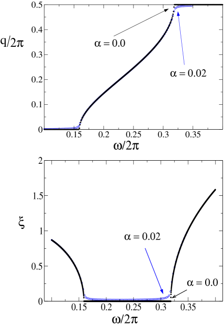
FIG. 1.: Wave vector $q$ and inverse of the decay length $\xi$ as functions of $\omega$ for two different values of the damping, $\alpha=0.02$ (open circles) and the Hamiltonian case $\alpha=0.0$ (filled ones). The coupling parameter $C$ is in both cases equal to $0.75$.

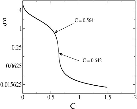
FIG. 2.: Inverse of the decay length (in logarithmic scale) as a function of the coupling parameter $C$, for a fixed value $\omega=3\omega_{b}$. We mark two values of $C$, $0.564$ and $0.642$, which correspond to two rather different values of $\xi$, also used in the next figure. The rest of the parameters are $\omega_{b}=0.2\pi$, $\alpha=0.02$ and $F_{ac}=0.02$.

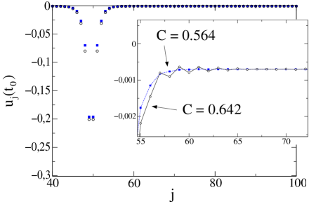
FIG. 3.: Breather profiles (two-site breathers) at a given time for two different values of $C$ ($0.564$ filled circles and $0.642$ open ones, see also the previous figure). The inset shows the right hand side tails, where we can observe the existence of a phonon in the second case, corresponding to the entrance of the third harmonic of $\omega_{b}$ in the phonon band. The points are connected as a guide to the eye.

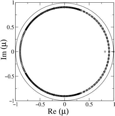
FIG. 4.: Floquet spectrum for the one-site breather near $C=0.5296$ and closely after the first pitchfork bifurcation. All eigenvalues are in a circle of radius $\exp(-\alpha t_{b}/2)$ except two, one of which crosses the unit circle by $+1$. The lower figure shows the profile of the eigenvector corresponding to this unstable eigenvalue (both velocity and position components, $\dot{\epsilon}_{i}$, $\epsilon_{i}$). Note that it is antisymmetric and strongly localized.

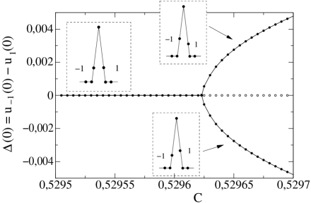
FIG. 5.: Profiles of the breather around the area of the pitchfork bifurcation.

FIG. 6.: Floquet spectrum for the Hopf bifurcation at $C=0.871$. An eigenvalue and its complex conjugate cross the unit circle at a non-zero angle in the complex plane. The figure at the bottom shows the corresponding eigenvector.

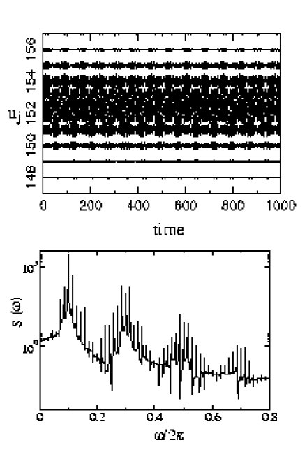
FIG. 7.: Two-site quasiperiodic breather. Note that particles on both sides of the breather are out of phase. The figure below shows the power spectrum of one of the central particles. The peaks are linear combinations of the two relevant frequencies, $\omega_{b}$ and $\omega_{\text{new}}$. Note that only odd harmonics of $\omega_{b}$ appear.

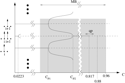
FIG. 8.: Scheme showing all bifurcations found in our model up to values of $C\approx 1$. The most relevant ones are probably the pitchforks which exchange stability between the one-site and the two-site breather ($C_{\text{P1}}$, $C_{\text{P2}}$). At $C=0.817$ the two-site breather has a subcritical Hopf bifurcation, connecting it to a quasiperiodic breather. At $C=0.88$ this quasiperiodic solution disappears as it turns into a slow moving breather. The grey-shaded areas between $C=0.51$ and $C=0.96$ are those where moving breathers, either fast or slow, can be found.

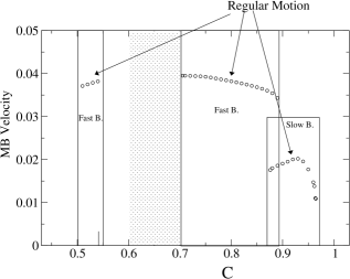
FIG. 9.: Velocity of MB vs. coupling parameter $C$. Dashed area shows the region in which MB have a diffusive motion. It is also showed different regions of “slow” and “fast” MB. See the text for details.

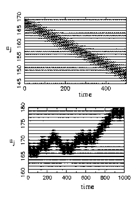
FIG. 10.: The upper figure shows a MB with regular motion at $C=0.75$. Below, a MB with diffusive motion at $C=0.65$.

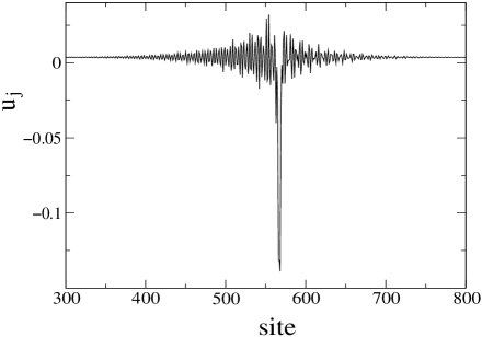
FIG. 11.: Instantaneous profile of a MB at $C=0.75$ and $F_{ac}=0.045$. Note the clear asymmetry of the phonon tails in front of and behind the breather.

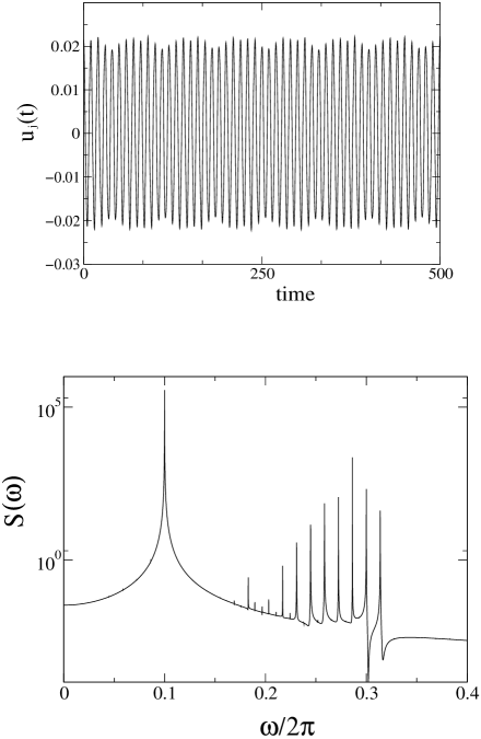
FIG. 12.: Time evolution for the tail of quasiperiodic breather at $C=0.817$ (upper figure) and the corresponding power spectrum (down figure) whose peaks are given by linear combinations of two frequencies $\omega_{b}$ and $\omega_{new}$.

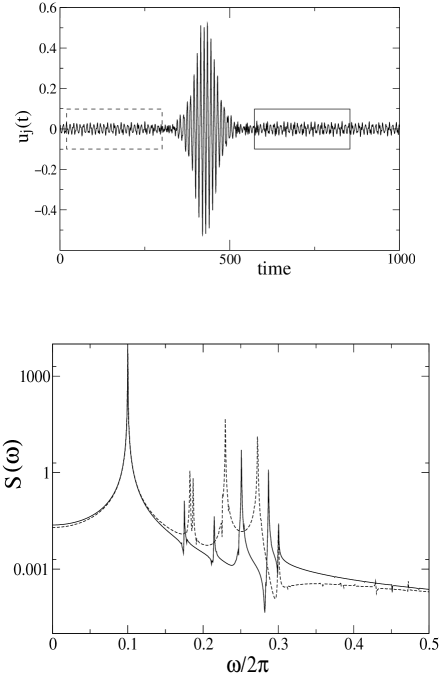
FIG. 13.: Time evolution for a particle which is passed by a MB (upper). Below, power spectra corresponding to the tails before and after the passage of the breather. Note how the peaks are shifted by Doppler effect.

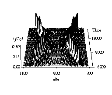
FIG. 14.: An elastic collision between two slowly moving breathers. It is possible to appreciate how the breathers “see” each other through their phonon tails. This collision was obtained at $C=0.89$.

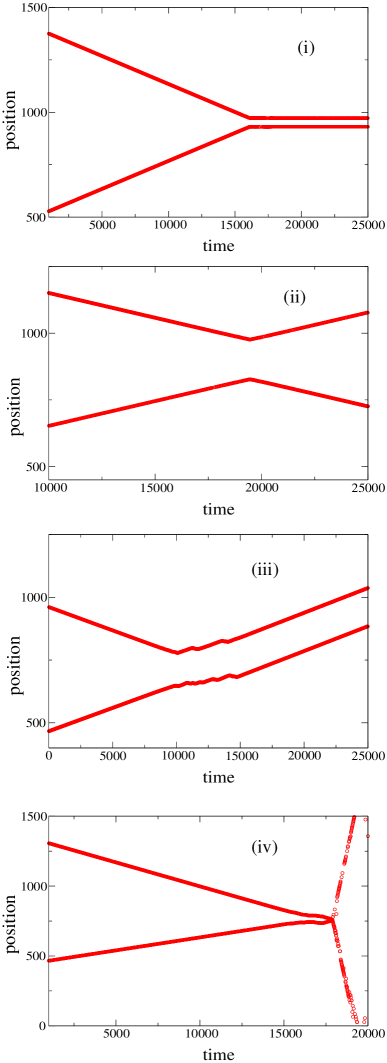
FIG. 15.: Four scenarios of collisions between breathers. We represent the traces by plotting the position of the energy maximum. (i) Formation of a pinned “molecule” after a collision of two MB at $C=0.75$ and $F_{ac}=0.011$. (ii) “elastic” collision at $C=0.89$ and $F_{ac}=0.02$. (iii) Formation of mobile “molecule” $C=0.89$ and $F_{ac}=0.02$. (iv) Annihilation of a “slow” and a “fast” breather at $C=0.89$ and $F_{ac}=0.02$. In this last case, the traces after the collision correspond to linear radiation (phonons).

REFERENCES

- [1] E. Trías, J. J. Mazo, and T. P. Orlando, Phys. Rev. Lett. 84, 741 (2000).
- [2] P. Binder et al., Phys. Rev. Lett. 84, 745 (2000).
- [3] P. Binder, D. Abraimov, and A. V. Ustinov, Phys. Rev. E 62, 2858 (2000).
- [4] U. T. Schwarz, L. Q. English, and A. J. Sievers, Phys. Rev. Lett. 83, 223 (1999).
- [5] S. Flach and C. R. Willis, Physics Reports 295, 181 (1998).
- [6] S. Aubry, Physica D 103, 201 (1997).
- [7] J.-A. Sepulchre and R. S. MacKay, Nonlinearity 10, 679 (1997).
- [8] R. S. MacKay and S. Aubry, Nonlinearity 7, 1623 (1994).
- [9] J. L. Marín and S. Aubry, Nonlinearity 9, 1501 (1996).
- [10] S. Watanabe, H. S. J. van der Zant, S. H. Strogatz, and T. Orlando, Physica D 97, 429 (1996).
- [11] V. I. Arnold, Mathematical Methods of Classical Mechanics, 2nd ed. (Springer, New York, 1989).
- [12] J. L. Marín and S. Aubry, Physica D 119, 163 (1998).
- [13] S. Flach and M. Spicci, J. Phys.: Condens. Matter 11, 321 (1999).
- [14] J. L. Marín, Intrinsic Localized Modes in Nonlinear Lattices (University of Zaragoza, Spain, 1997), also available at wanda.unizar.es.
- [15] T. Cretegny, S. Aubry, and S. Flach, Physica D 119, 73 (1998).
- [16] S. H. Strogatz, Nonlinear dynamics and chaos (Perseus Books, Reading, MA, 1994).
- [17] S. Aubry and T. Cretegny, Physica D 119, 34 (1998).
- [18] A. Katok and B. Hasselblatt, Introduction to the Modern Theory of Dynamical Systems (Cambridge University Press, Cambridge, U.K., 1995).
- [19] K. W. Sandusky, J. B. Page, and K. E. Schmidt, Phys. Rev. B 46, 6161 (1992).
- [20] K. Hori and S. Takeno, J. Phys. Soc. Jpn. 61, 2186 (1992).
- [21] K. Hori and S. Takeno, J. Phys. Soc. Jpn. 61, 4263 (1992).
- [22] S. Flach and K. Kladko, Physica D 127, 61 (1999).
- [23] J. C. Eilbeck and R. Flesch, Phys. Lett. A 149, 200 (1990).
- [24] D. B. Duncan, J. C. Eilbeck, H. Feddersen, and J. Wattis, Physica D 68, 1 (1993).
- [25] L. M. Floría and J. J. Mazo, Adv. Phys. 45, 505 (1996).
- [26] S. Flach and C. R. Willis, Phys. Rev. Lett. 72, 1777 (1994).
- [27] T. Ahn, R. S. MacKay, and J.-A. Sepulchre, Preprint (1999).
- [28] D. Chen, S. Aubry, and G. Tsironis, Phys. Rev. Lett. 77, 4776 (1996).
- [29] N. R. Quintero and A. Sánchez, Eur. Phys. J. B 6, 133 (1998).
- [30] P. S. Lomdahl and M. R. Samuelsen, Phys. Lett. A 128, 427 (1988).
- [31] E. Ott, Chaos in Dynamical Systems (Cambridge University Press, Cambridge, U.K., 1993).
- [32] L. D. Landau and E. M. Lifschitz, Fluid Mechanics, 2nd ed. (Pergamon, Oxford, 1982).
- [33] J. P. Boyd, Nonlinearity 3, 177 (1990).