Shape-Changing Collisions of Coupled Bright Solitons in Birefringent Optical Fibers

Abstract

We critically review the recent progress in understanding soliton propagation in birefringent optical fibers. By constructing the most general bright two-soliton solution of the integrable coupled nonlinear Schrödinger equation (Manakov model) we point out that solitons in birefringent fibers can in general change their shape after interaction due to a change in the intensity distribution among the modes eventhough the total energy is conserved. However the standard shape-preserving collision (elastic collision) property of the $(1+1)$ dimensional solitons is recovered when restrictions are imposed on some of the soliton parameters. As a consequence the following further properties can be deduced using this shape-changing collision.

(i) The exciting possibility of switching of solitons between orthogonally polarized modes of the birefringent fiber exists.

(ii) When additional effects due to periodic rotation of birefringence axes are considered, the shape changing collision can be used as a switch to suppress or to enhance the periodic intensity exchange between the orthogonally polarized modes.

(iii) For ultra short optical soliton pulse propagation in non-Kerr media, from the governing equation an integrable system of coupled nonlinear Schrödinger equation with cubic-quintic terms is identified. It admits a nonlocal Poisson bracket structure.

(iv) If we take the higher-order terms in the coupled nonlinear Schrödinger equation into account then their effect on the shape changing collision of solitons, during optical pulse propagation, can be studied by using a direct perturbational approach.

1. Introduction

The study of optical wave propagation in a nonlinear dispersive (dielectric) fiber has been receiving considerable attention in recent times as the fiber can support under suitable circumstances a stable pulse called optical soliton [1-3]. It arises essentially due to a compensation of the effect of dispersion of the pulse by the nonlinear response of the medium.

The analysis of such pulse propagation naturally starts from the Maxwell’s equations for electromagnetic wave propagation in a dielectric medium,

$$\nabla^{2}\overrightarrow{E}-\frac{1}{c^{2}}\frac{\partial^{2}\overrightarrow{E}}{\partial t^{2}}=-\mu_{0}\frac{\partial^{2}\overrightarrow{P}}{\partial t^{2}},$$ (1)

where the induced polarization for silica fibers is

$$\overrightarrow{P}(\overrightarrow{r},t)=\epsilon_{0}\left[\chi^{(1)}.\overrightarrow{E}\right.\\ \left.+\chi^{(3)}\vdots\overrightarrow{E}\overrightarrow{E}\overrightarrow{E}+...\right].$$

In equation(1), $\overrightarrow{E}$ represents the electric field, c is the velocity of light, $\mu_{0}$ and $\epsilon_{0}$ are the permeability and permitivity of free space respectively, $\chi^{(m)}$ is the mth order susceptibility tensor.

In order to analyse equation(1) it is necessary to make several simplifying assumptions: (i) The nonlinear part of the induced polarization is treated as a small perturbation to the linear part. (ii) The optical field is assumed to maintain its polarization along the fiber. (iii) Fiber loss is assumed to be very small. (iv) The nonlinear response of the fiber is assumed to be instantaneous. (v) In a slowly varying envelope approximation for pulse propagation along the fiber, the electric field can be written as [4]

$$\overrightarrow{E}(\overrightarrow{r},t)=\frac{1}{2}\overrightarrow{e}\Big{[}F(x,y)E(z,t)\\ e^{i(K_{0}z-\omega_{0}t)}+c.c\Big{]},$$

where c.c stands for complex conjugate, $\overrightarrow{e}$ is the unit polarization vector of the light assumed to be linearly polarized, E is the slowly varying electric field, $F(x,y)$ is the mode distribution function in the $(x,y)$ plane, while $K_{0}$ and $\omega_{0}$ denote the propagation constant and central frequency of the optical pulse respectively.

Under the above assumptions, rewriting equation(1) by using the method of separation of variables and introducing the coordinate system, $T$$=$$t$$-$$\frac{z}{v_{g}}$, moving with the pulse at the group-velocity $v_{g}$ = $\frac{\partial K}{\partial\omega}$, one can obtain a wave equation for the evolution of E as

$$i\frac{\partial E}{\partial z}-\frac{K^{\prime\prime}}{2}\frac{\partial^{2}E}{\partial T^{2}}+\gamma_{0}|E|^{2}E=0,$$ (2)

where $\gamma_{0}$$=$$\frac{n_{2}\omega_{0}}{cA_{eff}}$. Here $A_{eff}$ denotes the effective core area of the single-mode fiber, $n_{2}$ represents the nonlinear index coefficient and the parameter $K^{\prime\prime}=\left(\frac{\partial^{2}K}{\partial\omega^{2}}\right)_{\omega=\omega_{0}}=\frac{1}{v_{g}^{2}}$ accounts for the group velocity dispersion (GVD). After normalizing equation(4) and using the transformation, $q=\left[\frac{\gamma_{0}T_{0}^{2}}{|K^{\prime\prime}|}\right]^{\frac{1}{2}}E,\;\;\xi=\frac{z|K^{\prime\prime}|}{T_{0}^{2}},\;\;\tau=\frac{T}{T_{0}}$ and then redefining $\xi$ as z and $\tau$ as t we get the ubiquitous nonlinear Schrödinger (NLS) equation,

$$iq_{z}-(\mbox{sgn}\,K^{\prime\prime})q_{tt}+2|q|^{2}q=0,$$ (3)

in which $T_{0}$ represents the width of the incident pulse, z and t are the normalized distance and time along the direction of propagation and q is the normalized envelope. The NLS equation admits the familiar bright envelope (one) soliton

$$q(z,t)=\frac{k_{1R}exp\left[i\left(\left(k_{1R}^{2}-k_{1I}^{2}\right)z+k_{1I}t+\eta_{1I}^{(0)}\right)\right]}{\mbox{cosh}\left[k_{1R}\left(t-k_{1I}z+\eta_{1R}^{(0)}\right)\right]},$$ (4)

in the anamolous dispersion region $(K^{\prime\prime}<0)$, where $k_{1R}$ and $k_{1I}$ give the amplitude and velocity of the soliton respectively and $\eta_{1}^{(0)}$ is an arbitrary complex parameter. In the normal dispersion regime $(K^{\prime\prime}>0)$, equation(5) possesses dark soliton solutions [5]. Equation(5) is valid in the picosecond regime since in obtaining the above equation the optical field is assumed to be quasi-monochromatic. For ultra short pulses (width $\leq 100fs$) one has to include additional effects such as third order dispersion, nonlinear dispersion, self induced Raman effect, etc. Then equation(5) is for example replaced by the higher-order NLS (HNLS) equation,

$$iq_{z}-(\mbox{sgn}\,K^{\prime\prime})q_{tt}+2|q|^{2}q-\epsilon q_{ttt}-\lambda_{1}(|q|^{2}q)_{t}-\lambda_{2}|q|^{2}_{t}q=0.$$ (5)

Considerable attention has been paid to this HNLS equation which results from the delayed response of the fiber nonlinearity [6].

2. Electromagnetic Wave Propagation in Birefringent Fibers and the Coupled NLS Equation

In general a single mode fiber can support two distinct modes of polarization which are orthogonal to each other. This phenomenon is known as birefringence. Among these two modes one corresponds to the ordinary ray (O-ray) in which the refractive index of the medium is constant along every direction of the incident ray. The other is the extraordinary ray (E-ray) whose refractive index for the medium varies with the direction of the incident ray. In an ideal fiber these two modes are degenerate, while in a real fiber due to the fiber nonlinearity this degeneracy is broken and the phenomenon is known as “modal birefringence” [1].

Thus due to the effect of birefringence and nonlinear response of the medium there is a possibility of interaction of two copropagating modes. As a result of this the phase of one mode not only depends on its own intensity (Self Phase Modulation (SPM)) but also on the intensity of the copropagating mode (Cross Phase Modulation (XPM)) [1,2].

The propagation equation for such modes can be obtained again from the Maxwell’s equations by considering the electric field $\overrightarrow{E}$ in the slowly varying envelope approximation as

$$\overrightarrow{E}(\overrightarrow{r},t)=\frac{1}{2}\left[(\overrightarrow{e_{1}}E_{1}(z,t)e^{iK_{01}z}+\overrightarrow{e_{2}}E_{2}(z,t)\right.\left.e^{iK_{02}z})F(x,y)e^{-i\omega_{0}t}+c.c\right],$$ (6)

where $E_{1}$, $E_{2}$ are the amplitudes of two polarization components and $\overrightarrow{e}_{1}$, $\overrightarrow{e}_{2}$ are the unit orthonormal polarization vectors and $F(x,y)$ is the fiber mode distribution.

Proceeding in the same way as in the case of the single mode fiber one can obtain the following coupled system of equations for the envelopes of the two copropagating waves,

$$iE_{1z}+\frac{i}{v_{g1}}E_{1t}-\frac{K^{\prime\prime}}{2}E_{1tt}+\gamma_{0}(|E_{1}|^{2}+B|E_{2}|^{2})E_{1}=0,$$

$$iE_{2z}+\frac{i}{v_{g2}}E_{2t}-\frac{K^{\prime\prime}}{2}E_{2tt}+\gamma_{0}(|E_{2}|^{2}+B|E_{1}|^{2})E_{2}=0,$$ (7)

where z and t represent the normalized distance and time along the direction of propagation, $v_{g1}$ and $v_{g2}$ represent the group velocity of the two copropagating waves $E_{1}$ and $E_{2}$ respectively and $B=\frac{2+2\sin^{2}\vartheta}{2+\cos^{2}\vartheta}$ is the XPM coupling parameter ($\vartheta$ - birefringence ellipticity angle which varies between 0 and $\frac{\pi}{2}$ ). After suitable transformations as in the case of NLS equation we can rewrite the equation(9) in its normalized form as

$$iq_{1z}+q_{1tt}+2\mu(|q_{1}|^{2}+B|q_{2}|^{2})q_{1}=0,$$

$$iq_{2z}+q_{2tt}+2\mu(|q_{2}|^{2}+B|q_{1}|^{2})q_{2}=0.$$ (8)

The above equation is the coupled nonlinear Schrödinger (CNLS) equation which is in general nonintegrable. However for B$=$1 this reduces to the celebrated Manakov equations [7],

$$iq_{1z}+q_{1tt}+2\mu(|q_{1}|^{2}+|q_{2}|^{2})q_{1}=0,$$

$$iq_{2z}+q_{2tt}+2\mu(|q_{1}|^{2}+|q_{2}|^{2})q_{2}=0,$$ (9)

which is a completely integrable soliton system. The Lax pair for the Manakov system (11) can be identified as

$$L=\left(\begin{array}[]{ccc}-i\lambda&q_{1}&q_{2}\\ -q_{1}^{*}&i\lambda&0\\ -q_{2}^{*}&0&i\lambda\end{array}\right),\quad M=\left(\begin{array}[]{ccc}\{-2i\lambda^{2}+&\{2\lambda q_{1}&\{2\lambda q_{2}\\ i(|q_{1}|^{2}+|q_{2}|^{2})\}&+iq_{1t}\}&+iq_{2t}\}\\ \\ -2\lambda q_{1}^{*}+iq_{1t}^{*}&\{2i\lambda^{2}&-iq_{1}^{*}q_{2}\\ &-i|q_{1}|^{2}\}&\\ -2\lambda q_{2}^{*}+iq_{2t}^{*}&-iq_{1}q_{2}^{*}&\{2i\lambda^{2}\\ &&-i|q_{2}|^{2}\}\\ \end{array}\right),$$ (20)

such that

$$L_{z}-M_{t}+[L,M]=0,$$ (21)

which is equivalent to the Manakov equations (11). The existence of infinite number of involutive integrals of motion confirms the integrability of the Manakov system (11).

3. Bilinearization and Bright Two-Soliton Solution

In recent years to study the solution properties of the integrable systems several effective tools have been developed which include inverse scattering transform method, Hirota’s bilinearization method, Bäcklund transformation method, geometrical methods and so on. In this section by applying Hirota’s technique we point out that the most general bright one-soliton and two-soliton solutions for the Manakov system (11) can be obtained [8].

Considering equation (11) and by making the following bilinear transformation $q_{1}=\frac{g}{f}$, $q_{2}=\frac{h}{f}$, where g(z,t), h(z,t) are complex functions while f(z,t) is a real function, the following bilinear equations can be obtained,

$$(iD_{z}+D_{t}^{2})g.f=0,\;\;(iD_{z}+D_{t}^{2})h.f=0,\;\;D_{t}^{2}f.f=2\mu(gg^{*}+hh^{*}),$$ (22)

where $D_{z}$ and $D_{t}$ are Hirota’s bilinear operators. The above set of equations can be solved by making the following power series exapansion to g, h and f:

$$g=\lambda g_{1}+\lambda^{3}g_{3}+...,\;\;h=\lambda h_{1}+\lambda^{3}h_{3}+...,\;\;f=1+\lambda^{2}f_{2}+\lambda^{4}f_{4}+...,$$ (23)

where $\lambda$ is the formal expansion parameter. The resulting equations, after collecting the terms with the same power in $\lambda$, can be solved to obtain the forms of g, h and f. In order to get the one-soliton solution the power series expansions for g, h and f are terminated as follows, $g$$=$$\lambda g_{1}$, $h$$=$$\lambda h_{1}$ and $f$ $=$ $1$ $+$$\lambda^{2}f_{2}$. After following the procedure as mentioned before, the bright one-soliton solution is obtained as

$$\left(\begin{array}[]{c}q_{1}\\ q_{2}\end{array}\right)=\left(\begin{array}[]{c}\alpha\\ \beta\end{array}\right)\frac{e^{\eta_{1}}}{1+e^{\eta_{1}+\eta_{1}^{*}+R}}\;\;=\left(\begin{array}[]{c}A_{1}\\ A_{2}\end{array}\right)\frac{k_{1R}e^{i\eta_{1I}}}{\mbox{cosh}\,(\eta_{1R}+\frac{R}{2})},$$ (30)

where   $\eta_{j}=k_{j}(t+ik_{j}x)+\eta_{j}^{(0)},\;\;j=1,\;\;A_{1}=\frac{\alpha}{\Delta},\;\;A_{2}=\frac{\beta}{\Delta},\;\;\Delta=\sqrt{\mu(|\alpha|^{2}+|\beta|^{2})},$   $e^{R}=\frac{\mu(|\alpha|^{2}+|\beta|^{2})}{(k_{1}+k_{1}^{*})^{2}}$,   $\alpha$,  $\beta$, $k_{j}$ and $\eta_{j}^{(0)}$ are complex parameters. Here $\sqrt{\mu}(A_{1},A_{2})$ represents the unit polarization vector, $k_{1R}$ and $k_{1I}$ give the amplitude and velocity of the Manakov one soliton respectively.

For obtaining the bright two-soliton solution, the series is terminated as $g=\lambda g_{1}+\lambda^{3}g_{3},\;\;h=\lambda h_{1}+\lambda^{3}h_{3}$ and $f=1+\lambda^{2}f_{2}+\lambda^{4}f_{4}.$ After proceeding in a similar fashion as in the case of the one-soliton solution, the following bright two-soliton solution with six arbitrary complex parameters $k_{1}$, $k_{2}$, $\alpha_{1}$, $\beta_{1}$, $\alpha_{2}$ and $\beta_{2}$ can be obtained,

$$q_{1} = \frac{\alpha_{1}e^{\eta_{1}}+\alpha_{2}e^{\eta_{2}}+e^{\eta_{1}+\eta_{1}^{*}+\eta_{2}+\delta_{1}}+e^{\eta_{1}+\eta_{2}+\eta_{2}^{*}+\delta_{2}}}{D},$$

$$q_{2} = \frac{\beta_{1}e^{\eta_{1}}+\beta_{2}e^{\eta_{2}}+e^{\eta_{1}+\eta_{1}^{*}+\eta_{2}+\delta_{1}^{\prime}}+e^{\eta_{1}+\eta_{2}+\eta_{2}^{*}+\delta_{2}^{\prime}}}{D},$$ (31)

where

$$D = \displaystyle 1+e^{\eta_{1}+\eta_{1}^{*}+R_{1}}+e^{\eta_{1}+\eta_{2}^{*}+\delta_{0}}+e^{\eta_{1}^{*}+\eta_{2}+\delta_{0}^{*}}+e^{\eta_{2}+\eta_{2}^{*}+R_{2}}+e^{\eta_{1}+\eta_{1}^{*}+\eta_{2}+\eta_{2}^{*}+R_{3}},$$

$$e^{\delta_{0}} = \frac{\kappa_{12}}{k_{1}+k_{2}^{*}},\;\;e^{R_{1}}=\frac{\kappa_{11}}{k_{1}+k_{1}^{*}},\;\;\;\;e^{R_{2}}=\frac{\kappa_{22}}{k_{2}+k_{2}^{*}},$$

$$e^{\delta_{1}} = \frac{k_{1}-k_{2}}{(k_{1}+k_{1}^{*})(k_{1}^{*}+k_{2})}(\alpha_{1}\kappa_{21}-\alpha_{2}\kappa_{11}),\;\;e^{\delta_{2}}=\frac{k_{2}-k_{1}}{(k_{2}+k_{2}^{*})(k_{1}+k_{2}^{*})}(\alpha_{2}\kappa_{12}-\alpha_{1}\kappa_{22}),$$

$$e^{\delta_{1}^{{}^{\prime}}} = \frac{k_{1}-k_{2}}{(k_{1}+k_{1}^{*})(k_{1}^{*}+k_{2})}(\beta_{1}\kappa_{21}-\beta_{2}\kappa_{11}),\;\;e^{\delta_{2}^{{}^{\prime}}}=\frac{k_{2}-k_{1}}{(k_{2}+k_{2}^{*})(k_{1}+k_{2}^{*})}(\beta_{2}\kappa_{12}-\beta_{1}\kappa_{22}),$$

$$e^{R_{3}} = \frac{|k_{1}-k_{2}|^{2}}{(k_{1}+k_{1}^{*})(k_{2}+k_{2}^{*})|k_{1}+k_{2}^{*}|^{2}}(\kappa_{11}\kappa_{22}-\kappa_{12}\kappa_{21})\;\;\mbox{and}\;\;\kappa_{ij}=\frac{\mu(\alpha_{i}\alpha_{j}^{*}+\beta_{i}\beta_{j}^{*})}{k_{i}+k_{j}^{*}}.$$

The above most general bright two-soliton solution corresponds to a shape changing (inelastic) collision of two bright solitons which will be explained in the following sections.

4. Inelastic Collision and Switching of Bright Solitons in the Manakov Model

The collision property of bright solitons can be revealed by analysing the asymptotic form of the two-soliton solution [8]. Without loss of generality we assume that $k_{iR}>0\;\;\mbox{and}\;\;k_{1I}>k_{2I},$ where i=1,2, which corresponds to a head-on collision. One can easily check that asymptotically the two-soliton solution becomes two well separated solitons $S_{1}$ and $S_{2}$. Thus for the above condition, asymptotically the $\eta_{iR}$’s for the two-solitons become as (i)$\eta_{1R}\sim 0$, $\eta_{2R}\rightarrow\pm\infty$ as $z\rightarrow\pm\infty$ and  (ii)$\eta_{2R}\sim 0$, $\eta_{1R}\rightarrow\mp\infty$ as $z\rightarrow\pm\infty.$   This leads to the following asymptotic forms for the two-soliton solution.
(i)Limit z $\rightarrow-\infty$: (a) $S_{1}$ ($\eta_{1R}\sim 0,\;\;\eta_{2R}\rightarrow-\infty):$

$$\left(\begin{array}[]{c}q_{1}\\ q_{2}\end{array}\right)\rightarrow\left(\begin{array}[]{c}\alpha_{1}\\ \beta_{1}\end{array}\right)\frac{e^{\eta_{1}}}{1+e^{\eta_{1}+\eta_{1}^{*}+R_{1}}}=\left(\begin{array}[]{c}A_{1}^{1-}\\ A_{2}^{1-}\end{array}\right)k_{1R}e^{i\eta_{1I}}{\mbox{sech}\,\left(\eta_{1R}+\frac{R_{1}}{2}\right)},$$ (38)

where $(A_{1}^{1-},A_{2}^{1-})=[\mu(\alpha_{1}\alpha_{1}^{*}+\beta_{1}\beta_{1}^{*})]^{-\frac{1}{2}}(\alpha_{1},\beta_{1})$. Here superscript 1- denotes $S_{1}$ at the limit $z\rightarrow-\infty$ and subscripts 1 and 2 refer to the modes $q_{1}$ and $q_{2}$.

(b) $S_{2}$ ($\eta_{2R}\sim 0,\;\;\eta_{1R}\rightarrow\infty)$:

$$\left(\begin{array}[]{c}q_{1}\\ q_{2}\end{array}\right)\rightarrow\left(\begin{array}[]{c}e^{\delta_{1}-R_{1}}\\ e^{\delta_{1}^{\prime}-R_{1}}\end{array}\right)\frac{e^{\eta_{2}}}{1+e^{\eta_{2}+\eta_{2}^{*}+R_{3}-R_{1}}}=\left(\begin{array}[]{c}A_{1}^{2-}\\ A_{2}^{2-}\end{array}\right)k_{2R}e^{i\eta_{2I}}{\mbox{sech}\,\left(\eta_{2R}+\frac{(R_{3}-R_{1})}{2}\right)},$$ (39)

where $(A_{1}^{2-},A_{2}^{2-})=(\frac{a_{1}}{a_{1}^{*}})\;c\;[\mu(\alpha_{2}\alpha_{2}^{*}+\beta_{2}\beta_{2}^{*})]^{-\frac{1}{2}}\left[(\alpha_{1},\beta_{1})\kappa_{11}^{-1}-(\alpha_{2},\beta_{2})\kappa_{21}^{-1}\right]$ in which $a_{1}=(k_{1}+k_{2}^{*})\left[(k_{1}-k_{2})(\alpha_{1}^{*}\alpha_{2}+\beta_{1}^{*}\beta_{2})\right]^{\frac{1}{2}}$  and   $c=\left[\frac{1}{|\kappa_{12}|^{2}}-\frac{1}{\kappa_{11}\kappa_{22}}\right]^{-\frac{1}{2}}.$

(ii)Limit $z\rightarrow\infty$: (a) $S_{1}$ ($\eta_{1R}$ $\sim$0,   $\eta_{2R}$ $\rightarrow$ $\infty$):

$$\left(\begin{array}[]{c}q_{1}\\ q_{2}\end{array}\right)\rightarrow\left(\begin{array}[]{c}e^{\delta_{2}-R_{2}}\\ e^{\delta_{2}^{\prime}-R_{2}}\end{array}\right)\frac{e^{\eta_{1}}}{1+e^{\eta_{1}+\eta_{1}^{*}+R_{3}-R_{2}}}=\left(\begin{array}[]{c}A_{1}^{1+}\\ A_{2}^{1+}\end{array}\right)k_{1R}e^{i\eta_{1I}}{\mbox{sech}\,\left(\eta_{1R}+\frac{(R_{3}-R_{2})}{2}\right)},$$ (40)

where $(A_{1}^{1+},A_{2}^{1+})=(\frac{a_{2}}{a_{2}^{*}})\;c\;[\mu(\alpha_{1}\alpha_{1}^{*}+\beta_{1}\beta_{1}^{*})]^{-\frac{1}{2}}\left[(\alpha_{1},\beta_{1})\kappa_{12}^{-1}-(\alpha_{2},\beta_{2})\kappa_{22}^{-1}\right]$ in which $a_{2}=(k_{2}+k_{1}^{*})\left[(k_{1}-k_{2})(\alpha_{1}\alpha_{2}^{*}+\beta_{1}\beta_{2}^{*})\right]^{\frac{1}{2}}.$

(b) $S_{2}$ ($\eta_{2R}\sim 0,\;\;\eta_{1R}\rightarrow-\infty)$:

$$\left(\begin{array}[]{c}q_{1}\\ q_{2}\end{array}\right)\rightarrow\left(\begin{array}[]{c}\alpha_{2}\\ \beta_{2}\end{array}\right)\frac{e^{\eta_{2}}}{1+e^{\eta_{2}+\eta_{2}^{*}+R_{2}}}=\left(\begin{array}[]{c}A_{1}^{2+}\\ A_{2}^{2+}\end{array}\right)k_{2R}e^{i\eta_{2I}}{\mbox{sech}\,\left(\eta_{2R}+\frac{R_{2}}{2}\right)},$$ (47)

where $(A_{1}^{2+},A_{2}^{2+})=[\mu(\alpha_{2}\alpha_{2}^{*}+\beta_{2}\beta_{2}^{*})]^{-\frac{1}{2}}(\alpha_{2},\beta_{2})$.

In the above set of equations, the solitons before interaction are given by equations (18) and (19) and the solitons after interaction are given by equations (20) and (21). We observe from the above mentioned equations (18-21) that due to the interaction between two copropagating solitons $S_{1}$ and $S_{2}$, their amplitudes change from $(A_{1}^{1-}k_{1R},A_{2}^{1-}k_{1R})$ and $(A_{1}^{2-}k_{2R},A_{2}^{2-}k_{2R})$ to $(A_{1}^{1+}k_{1R},A_{2}^{1+}k_{1R})$ and $(A_{1}^{2+}k_{2R},A_{2}^{2+}k_{2R})$ respectively, in addition to a change in their phases by an amount $\frac{R_{3}-R_{1}-R_{2}}{2}$ and $\frac{-R_{3}+R_{1}+R_{2}}{2}$ respectively. The interesting behaviour which should be noted in this collision is that though the amplitude and phase of each soliton change during collision, the total intensity of each soliton is conserved, ie., $|A_{1}^{n\pm}|^{2}+|A_{2}^{n\pm}|^{2}=\frac{1}{\mu}$, where n=1,2 represent the solitons $S_{1}$ and $S_{2}$ respectively. Thus in such a collision there is a change in the distribution of intensity among the two component fields keeping the total intensity conserved. This is shown in Fig(1), where a head-on collision of two solitons is pictured for the parameter values, $k_{1}=1+i$, $k_{2}=2-i$, $\beta_{i}=1$, $\alpha_{1}=1$ and $\alpha_{2}=\frac{(39+i80)}{89}$. Here initially the time profiles of the two-solitons are evenly split between the two components $q_{1}$ and $q_{2}$. At the large positive z end the profile of the $S_{1}$ soliton is completely suppressed in the $q_{1}$ component while it is enhanced in the $q_{2}$ component. Noticeable changes in $S_{2}$ soliton also take place.

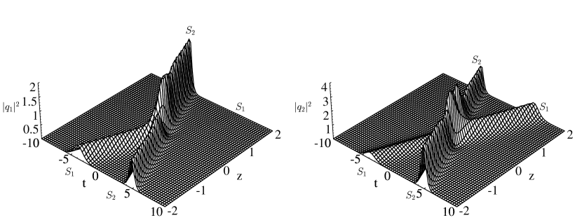
Fig. 1: Intensity profiles $|q_{1}|^{2}$ and $|q_{2}|^{2}$ of the head-on collision of the two-soliton solution of the Manakov model.

However we can regain the elastic collision for $\alpha_{2}=1$ [8]. Thus for the special case $\alpha_{1}:\alpha_{2}=\beta_{1}:\beta_{2}$ the standard elastic collision nature of the soliton can be obtained. The above analysis shows that the (1+1) dimensional soliton system given by equation(11) exhibits a novel type of shape changing collision not seen in any other (1+1) dimensional evolution equation which led us to identify the exciting possibility of switching of solitons between modes by changing the phase [8]. This novel type of interaction led Jakubowski et al. to suggest a method for implementing computation in a bulk nonlinear medium without interconnecting discrete components [9].

5. Periodically Twisted Birefringent Fibers and Soliton Interaction

Soliton propagation in a periodically twisted birefringent fiber has gained considerable attention recently [1,10]. The effect of periodic twist on the soliton propagation can be described by the coupled wave equations of the form

$$iq_{1z}+q_{1tt}+\varrho q_{1}+\sigma q_{2}+2\mu(|q_{1}|^{2}+|q_{2}|^{2})q_{1} = 0,$$

$$iq_{2z}+q_{2tt}-\varrho q_{2}+\sigma q_{1}+2\mu(|q_{1}|^{2}+|q_{2}|^{2})q_{2} = 0,$$ (48)

where $\sigma$ and $\varrho$ are the normalized linear coupling constants caused by the periodic twist of the birefringence axes and the phase-velocity mismatch from resonance respectively. It can be easily verified that the transformation, $q_{1}=\cos\theta e^{i\Gamma z}q_{1M}-\sin\theta e^{-i\Gamma z}q_{2M},\;\;q_{2}=\sin\theta e^{i\Gamma z}q_{1M}+\cos\theta e^{-i\Gamma z}q_{2M},$ where the subscript M refers to the Manakov model and $\Gamma=\sqrt{\varrho^{2}+\sigma^{2}}$ and $\theta=\frac{1}{2}tan^{-1}(\frac{\sigma}{\varrho})$, reduces equation(22) to the coupled system given by equation(11). Hence by making use of the solutions (16) and (17) we obtain the one-soliton and two-soliton solutions of equation(22) respectively as

$$q_{1} = \left\{\cos\theta e^{i\Gamma z}A_{1M}-\sin\theta e^{-i\Gamma z}A_{2M}\right\}q_{c},$$

$$q_{2} = \left\{\sin\theta e^{i\Gamma z}A_{1M}+\cos\theta e^{-i\Gamma z}A_{2M}\right\}q_{c},$$ (49)

where $q_{c}=k_{1R}\exp(i\eta_{1I})\mbox{sech}\,(\eta_{1R}+\frac{R}{2})$ and

$$q_{1} = \frac{\left[\cos\theta e^{i\Gamma z}\alpha_{1}-\sin\theta e^{-i\Gamma z}\beta_{1}\right]e^{\eta_{1}}+\left[\cos\theta e^{i\Gamma z}\alpha_{2}-\sin\theta e^{-i\Gamma z}\beta_{2}\right]e^{\eta_{2}}}{D}$$ (50)

$$+\frac{\left[\cos\theta e^{i\Gamma z+\delta_{1}}-\sin\theta e^{-i\Gamma z+\delta_{1}^{\prime}}\right]e^{\eta_{1}+\eta_{1}^{*}+\eta_{2}}}{D}$$

$$+\frac{\left[\cos\theta e^{i\Gamma z+\delta_{2}}-\sin\theta e^{-i\Gamma z+\delta_{2}^{\prime}}\right]e^{\eta_{1}+\eta_{2}+\eta_{2}^{*}}}{D},$$

where all the parameters in (23) and (24) as well as the quantity D are defined in the previous section and $q_{2}$ can be obtained by just replacing $\cos\theta$ by $\sin\theta$ and $\sin\theta$ by $-\cos\theta$ in the above equation. The soliton interaction for this system can be studied by carrying out the asymptotic analysis as before.

Then the form of $S_{1}$ and $S_{2}$ before interaction ($z\rightarrow-\infty$) is given by

$$(q_{1},q_{2})=\left([\cos\theta e^{i\Gamma z}A_{1}^{1-}-\sin\theta e^{-i\Gamma z}A_{2}^{1-}],[\sin\theta e^{i\Gamma z}A_{1}^{1-}+\cos\theta e^{-i\Gamma z}A_{2}^{1-}]\right)q^{1-}$$

and

$$(q_{1},q_{2})=\left([\cos\theta e^{i\Gamma z}A_{1}^{2-}-\sin\theta e^{-i\Gamma z}A_{2}^{2-}],[\sin\theta e^{i\Gamma z}A_{1}^{2-}+\cos\theta e^{-i\Gamma z}A_{2}^{2-}]\right)q^{2-}$$

respectively, where $q^{1-}=k_{1R}exp(i\eta_{1I})\mbox{sech}(\eta_{1R}+\frac{R_{1}}{2})$, $q^{2-}=k_{2R}exp(i\eta_{2I})\mbox{sech}(\eta_{2R}+\frac{(R_{3}-R_{1})}{2})$ and the polarization vectors $A_{i}^{j-},$ j=1,2 are the same as in equations(18,19).

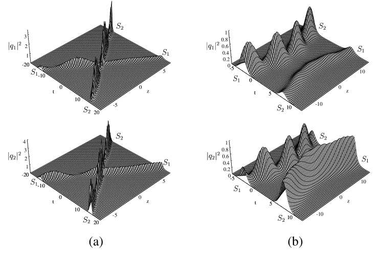
Fig. 2: (a) Evolution of the intensity profiles $|q_{1}|^{2}$ and $|q_{2}|^{2}$ showing the suppression in switching between the two modes of $S_{1}$ soliton in a twisted birefringent fiber. (b) Evolution of the intensity profiles $|q_{1}|^{2}$ and $|q_{2}|^{2}$ showing the suppression in switching of $S_{1}$ soliton and enhancement in $S_{2}$ soliton in a twisted birefringent fiber.

Proceeding in a similar fashion the form of $S_{1}$ and $S_{2}$ after interaction (limit z$\rightarrow\infty$) can be obtained as

$$(q_{1},q_{2})=\left([\cos\theta e^{i\Gamma z}A_{1}^{1+}-\sin\theta e^{-i\Gamma z}A_{2}^{1+}],[\sin\theta e^{i\Gamma z}A_{1}^{1+}+\cos\theta e^{-i\Gamma z}A_{2}^{1+}]\right)q^{1+}$$

and

$$(q_{1},q_{2})=\left([\cos\theta e^{i\Gamma z}A_{1}^{2+}-\sin\theta e^{-i\Gamma z}A_{2}^{2+}],[\sin\theta e^{i\Gamma z}A_{1}^{2+}+\cos\theta e^{-i\Gamma z}A_{2}^{2+}]\right)q^{2+}$$

respectively, where $q^{1+}=k_{1R}exp(i\eta_{1I})\mbox{sech}\left(\eta_{1R}+\frac{(R_{3}-R_{1})}{2}\right)$, $q^{2+}=k_{2R}exp(i\eta_{2I})\mbox{sech}(\eta_{2R}+\frac{R_{2}}{2})$ and the polarization vectors $A_{i}^{j+}$,i,j=1,2 are defined in section-4.

In order to facilitate the understanding of the above behaviour with reference to the optical soliton switching between the orthogonally polarized modes, it is convinient to obtain the oscillating part of the intensities associated with the above asymptotic forms as $\left|\frac{q_{l}(z,t)}{q^{n\mp}(z,t)}\right|^{2}=|A_{l}^{n\mp}|^{2}\cos^{2}\theta+|A_{j}^{n\mp}|^{2}\sin^{2}\theta+(-1)^{l}|A_{l}^{n\mp}||A_{j}^{n\mp}|\sin 2\theta\cos(2\Gamma z+\phi^{n\mp}),\;l,j=1,2,$ where $(l\neq j),$ $\phi^{n\mp}=\displaystyle\tan^{-1}\left(\frac{A_{1I}^{n\mp}}{A_{1R}^{n\mp}}\right)-\tan^{-1}\left(\frac{A_{2I}^{n\mp}}{A_{2R}^{n\mp}}\right).$ Now let us analyse how the presence of the oscillatory term in the above expression and the changes in $A_{j}^{n\pm}$ affect the switching dynamics of the solitons $S_{1}$ and $S_{2}$.

case(i): For all the $A_{j}^{n\pm}$’s are non zero, there is a periodic intensity switching which is always present in both the solitons and in both the components before as well as after the interaction.

case(ii): If any one of the $A_{j}^{n\pm}$’s is zero, and others are nonzero then soliton interaction suppresses or enhances switching dynamics. This is illustrated in Fig(2a), for the parameter values $k_{1}=1+i$, $k_{2}=2-i$, $\alpha_{1}=\beta_{1}=\beta_{2}=1$, $\alpha_{2}=\frac{(39+i80)}{89}$, $\rho=0.25$ and $\sigma=0.5$. Here we observe that for $|A_{1}^{1+}|\sim 0$ the switching in the intensity of soliton $S_{1}$ is fully suppressed in both the modes $q_{1}$ and $q_{2}$.

case(iii): If any two of the $A_{j}^{n\pm}$’s are zero then the soliton interaction suppresses and enhances switching dynamics. This can be verified from the Fig(2b), for the chosen parameters, $k_{1}=1+i(0.1)$, $k_{2}=1-i(0.1)$, $\alpha_{1}=0.86+i(0.5)$, $\alpha_{2}=0.5+i(0.86)$,  $\beta_{1}=0.7+i(0.72)$, $\beta_{2}=0.44+i(0.9)$ and $\rho=\sigma=0.25$. Thus for this case due to the interaction there is an exchange of periodic intensity between the two modes of soliton $S_{2}$ with the suppression of the switching dynamics in soliton $S_{1}$.

6. CNLS with Coupled Cubic-Quintic Nonlinearity

The model for ultra short optical pulse propagation in non-Kerr media (in particular materials with high nonlinear coefficients even at moderate optical intensities, for example, semiconductor dopped glasses, organic polymers, etc.) can be obtained by expanding the induced polarization vector in Maxwell’s equation(1) as

$$\overrightarrow{P}(\overrightarrow{r},t)=\epsilon_{0}[\chi^{(1)}.\overrightarrow{E}+\chi^{(3)}\vdots\overrightarrow{E}\overrightarrow{E}\overrightarrow{E}+\chi^{(5)}\dot{\dot{\vdots}}\overrightarrow{E}\overrightarrow{E}\overrightarrow{E}\overrightarrow{E}\overrightarrow{E}+...],$$ (51)

where $\chi^{(5)}$ is the fifth order nonlinear susceptibility and following the procedure as in the case of NLS equation. The resulting equation, in normalized form, describing the effects of quintic nonlinearity on the ultra short optical soliton pulse propagation is [11],

$$iq_{z}+q_{tt}+2|q|^{2}q+\gamma|q|^{4}q+i\gamma_{1}q_{ttt}+i\gamma_{2}(|q|^{2}q)_{t}+i\gamma_{3}(|q|^{4}q)_{t}=0.$$ (52)

The generalization of equation(26) in order to include multimode effects leads to the following coupled cubic-quintic NLS equation[11], after neglecting third order terms,

$$iq_{1z}+q_{1tt}+2(|q_{1}|^{2}+|q_{2}|^{2})q_{1}+(\rho_{1}|q_{1}|^{2}+\rho_{2}|q_{2}|^{2})^{2}q_{1}+2\rho_{2}[(\tau_{1}-\rho_{1})|q_{1}|^{2}\qquad$$

$$+(\tau_{2}-\rho_{2})|q_{2}|^{2}]\left|q_{2}\right|^{2}q_{1}-2i[(\rho_{1}|q_{1}|^{2}+\rho_{2}|q_{2}|^{2})q_{1}]_{t}+2i(\rho_{1}q_{1}^{*}q_{1t}+\rho_{2}q_{2}^{*}q_{2t})q_{1} = 0,$$

$$iq_{2z}+q_{2tt}+2(|q_{1}|^{2}+|q_{2}|^{2})q_{2}+(\tau_{1}|q_{1}|^{2}+\tau_{2}|q_{2}|^{2})^{2}q_{2}+2\tau_{1}[(\rho_{1}-\tau_{1})|q_{1}|^{2}\qquad$$

$$+(\rho_{2}-\tau_{2})|q_{2}|^{2}]\left|q_{1}\right|^{2}q_{2}-2i[(\tau_{1}|q_{1}|^{2}+\tau_{2}|q_{2}|^{2})q_{2}]_{t}+2i(\tau_{1}q_{1}^{*}q_{1t}+\tau_{2}q_{2}^{*}q_{2t})q_{2} = 0,$$

where $\rho_{1},\rho_{2},\tau_{1}$ and $\tau_{2}$ are real free parameters. The integrable nature of the above equation can be studied by obtaining the Lax pairs and conserved quantities for it. The Lax pair associated with equation(27) is

$$L=\left(\begin{array}[]{ccc}-i\lambda&q_{1}&q_{2}\\ -q_{1}^{*}&\ -i\theta_{1t}+i\lambda&0\\ -q_{2}^{*}&0&-i\theta_{2t}+i\lambda\end{array}\right),\;\;M=\left(\begin{array}[]{ccc}-2i\lambda^{2}&2\lambda q_{1}&2\lambda q_{2}\\ +i(|q_{1}|^{2}&+iq_{1t}&+iq_{2t}\\ +|q_{2}|^{2})&+\theta_{1t}q_{1}&+\theta_{2t}q_{2}\\ \\ -2\lambda q_{1}^{*}&2i\lambda^{2}&-iq_{1}^{*}q_{2}\\ +iq_{1t}^{*}&-i|q_{1}|^{2}&\\ -\theta_{1t}q_{1}^{*}&-i\theta_{1z}&\\ \\ -2\lambda q_{2}^{*}&-iq_{1}q_{2}^{*}&2i\lambda^{2}\\ +iq_{2t}^{*}&&-i|q_{2}|^{2}\\ -\theta_{2t}q_{2}^{*}&&-i\theta_{2z}\end{array}\right),$$ (68)

where $\theta_{1}=\int^{t}_{-\infty}(\rho_{1}|q_{1}|^{2}+\rho_{2}|q_{2}|^{2})dt^{\prime}$, $\theta_{2}=\int^{t}_{-\infty}(\tau_{1}|q_{1}|^{2}+\tau_{2}|q_{2}|^{2})dt^{\prime}$ and $\lambda$ is the spectral parameter. The compatability condition $L_{z}-M_{t}+[L,M]=0$ leads to equation(27). Though the integrable system(27) possesses infinite number of conserved quantities, only the lower ones are of physical importance. They can be written as

$$c_{1} = -{1\over 2i}\int_{-\infty}^{+\infty}dt(|q_{1}|^{2}+|q_{2}|^{2}),$$

$$c_{2} = -{i\over 4}\int_{-\infty}^{+\infty}dt[-i(q_{1}q_{1t}^{*}+q_{2}q_{2t}^{*})+\rho_{1}|q_{1}|^{4}+\tau_{2}|q_{2}|^{4}$$

$$+(\rho_{2}+\tau_{1})|q_{1}|^{2}|q_{2}|^{2}],$$

$$c_{3} = -{i\over 8}\int_{-\infty}^{+\infty}dt[(q_{1}q_{1tt}^{*}+q_{2}q_{2tt}^{*})+(|q_{1}|^{2}+|q_{2}|^{2})^{2}+i(|q_{1}|^{2}N_{1t}+|q_{2}|^{2}N_{2t})$$ (69)

$$+2i(N_{1}q_{1}q_{1t}^{*}+N_{2}q_{2}q_{2t}^{*})-(N_{1}^{2}|q_{1}|^{2}+N_{2}^{2}|q_{2}|^{2})],$$

etc., where $N_{1}=\theta_{1t}=\rho_{1}|q_{1}|^{2}+\rho_{2}|q_{2}|^{2}$ and $N_{2}=\theta_{2t}=\tau_{1}|q_{1}|^{2}+\tau_{2}|q_{2}^{2}|$. Here $c_{1}$, $c_{2}$ and $c_{3}$ may be related to the number operator, angular momentum and the Hamiltonian (energy) of the system(27) respectively. It is intriguing to note that the fields $q_{a}$ and $q_{a}^{*}$, a=1,2 do not have canonical Poisson bracket relations. However under the following nonultralocal Poisson bracket structure,

$$\{q_{1}(x),q^{*}_{1}(y)\} = \delta(x-y)+i\rho_{1}\epsilon(x-y)q_{1}(x)q^{*}_{1}(y),$$

$$\{q_{1}(x),q_{1}(y)\} = i\rho_{1}\epsilon(y-x)q_{1}(x)q_{1}(y),$$

$$\{q_{1}(x),q_{2}(y)\} = -i(\rho_{2}\theta(x-y)-\tau_{1}\theta(y-x))q_{1}(x)q_{2}(y),$$

$$\{q_{1}(x),q_{2}^{*}(y)\} = i(\rho_{2}\theta(x-y)-\tau_{1}\theta(y-x))q_{1}(x)q_{2}^{*}(y),$$ (70)

etc., where $\epsilon(x)=\theta(x)-\theta(-x)$ is the sign function defined through the step function, $\theta(x)=1$ for $x>0$, $\theta(x)=0,$ for $x\leq 0$, the integrals(29) become involutive. The interrelation between equation(27) and the Manakov system allows us to construct the soliton solution of equation(27) in terms of the known Manakov soliton solution.The fields of these two models are related through a

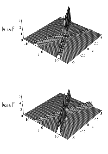
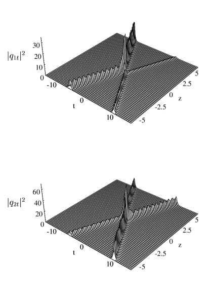
(a)                                                             (b)

Fig. 3: (a) Evolution of the intensity profiles $|q_{1Mt}|^{2}$ and $|q_{2Mt}|^{2}$ of the two-soliton solution of the Manakov model. (b) Intensity profiles $|q_{1t}|^{2}$ and $|q_{2t}|^{2}$ of the two-soliton solution of (27) for $\rho_{1}=\rho_{2}=\tau_{1}=\tau_{2}=1.$

nonlinear transformation for the dependent variables given by

$$q_{aM}=q_{a}exp(-i\theta_{a}),\;\;a=1,2$$ (71)

and the subscrip M represents the Manakov model. Their Lax pairs are related through a local gauge transformation $L^{\prime}=g^{-1}Lg-g^{-1}g_{t}$, $M^{\prime}=g^{-1}Mg-g^{-1}g_{x}$ where

$$g=\left[\begin{array}[]{ccc}1&0&0\\ 0&exp(-i\theta_{1})&0\\ 0&0&exp(-i\theta_{2})\end{array}\right].$$ (75)

Then the one-soliton solution takes the form

$$(q_{1},q_{2})=(\alpha e^{i\delta_{1}\tanh(\nu(t-vz+\delta))},\beta e^{i\delta_{2}\tanh(\nu(t-vz+\delta))})sech(\nu(t-vz+\delta))e^{i(\kappa t+\omega z)}$$ (76)

and the two-soliton solution can be obtained by substituting the two-soliton solution of the Manakov model in the transformation(31).

The effect of the dependence of phase change on the real free parameters $\rho_{1}$, $\rho_{2}$, $\tau_{1}$ and $\tau_{2}$ during collision can be revealed by carrying out the asymptotic analysis of the two-soliton solution as earlier. In this connection, we have taken the derivatives of the $|q_{j}^{n\mp}|,$ n,j=1,2, since the effect of the phases are reflected only in such terms rather than $|q_{j}^{n\mp}|^{2}$.

We have shown these effects for the parameter values $k_{1}=1.5+i(0.5),$ $k_{2}=2-i(0.7)$, $\alpha_{1}=\beta_{1}=\beta_{2}=1$ and $\alpha_{2}=\frac{39+i80}{89}$, by comparing the plots of the intensity profiles in the absence of the free parameters ($\rho_{1}$, $\rho_{2}$, $\tau_{1}$ and $\tau_{2}$) with those in their presence. It is obvious from equation(31) that for the choice of parameters $\rho_{1}$=$\rho_{2}$=$\tau_{1}$=$\tau_{2}$$=0$, the two-soliton solution of equation(27) reduces to that of the Manakov system. Hence in Figure(3a) we have plotted the intensity profiles of $|q_{1Mt}|^{2}$ and $|q_{2Mt}|^{2}$ for the above parametric values. In the figure there appears a splitting in each of the asymptotic profiles before and after interaction.

After setting $\rho_{1}$=$\rho_{2}$=$\tau_{1}$=$\tau_{2}$$=1$, we can show that the splitting disappears as shown in Figure(3b). Thus in addition to the inelastic soliton collision, there is a change in the asymptotic form (suppression of splitting) of the intensity profiles which arises due to the presence of the phase terms $\theta_{a}$ in the transformation(31).

7. General Soliton Perturbation

As mentioned in section(2) the CNLS equation is in general a nonintegrable one. We can apply the multiple scale perturbation theory to study such nonintegrable system with more general perturbations $R_{1}$ and $R_{2}$ as given below,

$$iq_{1z}+q_{1tt}+2\mu(|q_{1}|^{2}+|q_{2}|^{2})q_{1}=i\epsilon R_{1}(q_{1},q_{2},q_{1t},q_{2t}...),$$

$$iq_{2z}+q_{2tt}+2\mu(|q_{2}|^{2}+|q_{1}|^{2})q_{2}=i\epsilon R_{2}(q_{1},q_{2},q_{1t},q_{2t}...).$$ (77)

In the absence of the perturbation the above equation reduces to the Manakov system. After expanding $q_{i}$ as

$$q_{i}=q_{i}^{(0)}(k_{iR},k_{iI},A_{i}^{j\pm},\Phi_{i}^{j\pm})+\epsilon q_{i}^{(1)}+\epsilon^{2}q_{i}^{(2)}+...\;\mbox{i, j=1,2,}$$ (78)

where $A_{i}^{j\pm}$ and $\Phi_{i}^{j\pm}$ are the real and imaginary parts of the polarization vectors of the two-solitons respectively, in the asymptotic limits $z\rightarrow\pm\infty$. Substitution of this in equation(34), it is trivial to verify that $q_{i}^{(0)}$ is nothing but the two-soliton solution of the Manakov system. Asymptotically this two-soliton solution of the Manakov model given by equation(17) can be written as a combination of two one-solitons as $z\rightarrow\pm\infty$

$$\left(\begin{array}[]{c}q_{1}\\ q_{2}\end{array}\right)\rightarrow\left(\begin{array}[]{c}q_{1}^{1\pm}+q_{1}^{2\pm}\\ q_{2}^{1\pm}+q_{2}^{2\pm}\end{array}\right).$$ (83)

By using a direct perturbational approach [12] the evolution equations for the soliton parameters in the presence of perturbations can be obtained. Applying this method to CNLS equation(10) one can easily check that there occurs transmission and reflection scenarios during collision with a sensitive dependence of the collision outcome on the  cross phase modulation coefficient and initial soliton parameters. As a special case by taking $R_{i}=(-\gamma q_{i}+\bar{\beta}|q_{j}|^{2}q_{i}+\frac{\delta}{2}q_{itt})$ where i,j=1,2 we have studied the effect of perturbations such as fiber loss, dispersion gain and nonlinear gain. The importance of taking such a form for perturbation is that in the absence of $q_{1}$ and $q_{2}$ equation(34) along with the above specified form of $R_{1}$ and $R_{2}$ reduces to the Ginzburg-Landau equation governing pulse propagation in fiber amplifiers [1]. Since we have taken the asymptotic form of the more general two-soliton solution as the zeroth order solution, the collision properties of the system(34) can be directly studied by comparing the evolution of the soliton parameters in the limits $z\rightarrow-\infty$ and $z\rightarrow\infty$. We expect that this may lead to some novel results such that collision among the solitons may be used to compensate fiber loss experienced by the interacting coupled one-solitons corresponding to any one of the polarized modes.

8. Acknowledgement

This work is supported by the Department of Science and Technology, Government of India in the form of a Research Project.

References

- [1] G.P. Agarwal, Nonlinear Fiber Optics, 2nd ed., Academic Press, New York 1995.
- [2] N. Akhmediev and A. Ankiewicz, Solitons Nonlinear Pulses and Beams, Chapman and Hall, London 1997.
- [3] E. Iannone, F. Matera, A. Mecozzi and M.Settembre, Nonlinear Optical Communication Networks, Wiley-Interscience, New York 1998.
- [4] A. W. Snyder and J. Love, Optical Waveguide Theory, Chapman and Hall, London, 1983.
- [5] Y. S. Kivshar and H.Luther-Davies : Phys. Rep. 298, 81 (1998).
- [6] R. Radhakrishnan and M. Lakshmanan: Phys. Rev. E 54, 2949 (1996).
- [7] S. V. Manakov: Zh. Eksp. Teor. fiz 65, 505 (1973) [Sov. Phys. JETP 38, 248 (1974)].
- [8] R. Radhakrishnan, M. Lakshmanan and J. Hietarinta: Phys. Rev. E 56, 2 (1997).
- [9] M. H. Jakubowski, K. Steiglitz and R. Squiere: Phys. Rev. E 58, 6752 (1998).
- [10] R. Radhakrishnan and M. Lakshmanan: Phys. Rev. E 60, 2 (1999) in press.
- [11] R. Radhakrishnan, A.Kundu and M. Lakshmanan: Phys. Rev. E 60, 3 (1999) in press.
- [12] Y. Kodama and M. J. Ablowitz: Stud. Appl. Math 64, 225 (1981).