On the conditions for synchronization in unidirectionally coupled chaotic oscillators

Abstract

The conditions for synchronization in unidirectionally coupled chaotic oscillators are revisited. We demonstrate with typical examples that the conditional Lyapunov exponents (CLEs) play an important role in distinguishing between intermittent and permanent synchronizations, when the analytic conditions for chaos synchronization are not uniformly obeyed. We show that intermittent synchronization can occur when CLEs are very small positive or negative values close to zero while permanent synchronization occurs when CLEs take sufficiently large negative values. There is also strong evidence for the fact that for permanent synchronization the time of synchronization is relatively low while it is high for intermittent synchronization.

I Introduction

Much attention has been focussed on the synchronization of chaotic systems through different coupling schemes during the past decade or so. It has potential applications not only in secure communication but also in chaotic cryptographyvaidya0 . In order to achieve synchronization, coupled chaotic systems have to satisfy certain conditions. According to Pecora and Carroll the coupled chaotic systems can be regarded as master and slave systems which will perfectly synchronize only if the sub-Lyapunov or conditional Lyapunov exponents (CLEs) are all negativepecora1 ; pecora2 . However, recently there are reports claiming that synchronization can be achieved even with positive CLEsshuai ; guemez ; gutierrez . Also there are situations where one can observe intermittent or round-off induced synchronization phenomenonbaker ; baker2 ; zhou where locking occurs at certain time intervals only, so that the synchronization of chaos need not be always permanent. It is therefore important to understand clearly the conditions under which chaos synchronization can occur and to know how to distinguish between permanent and intermittent synchronizations exhibited by coupled chaotic systems.

In this paper, the analytic conditions for synchronization in coupled chaotic systems are revisited to show the difficulties in distinguishing between intermittent and permanent synchronizations which we illustrate by using simple chaotic systems. We demonstrate that the conditional Lyapunov exponents (CLEs) play an important role in distinguishing between intermittent and permanent synchronization, when the analytic conditions for chaos synchronization are not uniformly obeyed. We also point out that intermittent synchronization can occur when the largest CLE has a value close to zero (either positive or negative) while permanent synchronization occurs for sufficiently large negative values of the CLEs.

In Sec. II, we describe briefly the notion of chaos synchronization and the analytic conditions for synchronization which are to be uniformly obeyed as well as the existence of negative conditional Lyapunov exponents, with reference to a simple coupled system of autonomous Duffing-van der Pol (ADVP) oscillatorslakshman ; murali1 . Sec. III describes how the CLEs can be used to analyse the nature of synchronization in coupled ADVP oscillators. In Sec. IV, we show how conditional Lyapunov exponents play an important role in distinguishing between the intermittent and permanent synchronizations occurring in a class of unidirectionally coupled nonlinear oscillators including coupled chaotic pendulabaker , coupled Duffing oscillatorsbaker and coupled Murali-Lakshmanan-Chua (MLC) circuitslakshman either in the absence of the analytic criteria or when they are not uniformly obeyed. We also show how the time of synchronization can be used qualitatively to check the presence or absence of intermittent synchronization. Sec. V summarizes the results.

II Chaos synchronization and the conditions

In this section, we consider a set of two unidirectionally coupled autonomous Duffing-van der Pol (ADVP) oscillators as a model system to analyse the concept of chaos synchronization. Further, we show that the derived analytic conditions for the occurrence of chaos synchronization are uniformly obeyed in this system for a specific set of parametric values (that is, the analytic conditions are shown to be valid for all values of the variables, say, ($x_{1},x_{2},x_{3})\in{\cal R}^{3}$ for all $t$). We also indicate that when the usual analytic conditions are not uniformly obeyed by a given system, then it may either exhibit intermittent or permanent synchronizationbaker . In this case, the nature of the conditional Lyapunov exponents can be used profitably to distinguish between intermittent and permanent synchronization.

Figure 1: Figure showing the variation of synchronization error $\eta$ as time elapses in ADVP oscillators [Eqs. (1)] for $\nu=100$, $\alpha=0.35$, $\beta=300$ and $\varepsilon=1.35$.

We consider the ADVP model in which Murali and Lakshmanan demonstrated chaos synchronization lakshman ; murali1 . The rescaled and dimensionless version of the unidirectionally coupled ADVP oscillators can be written as

$$\dot{x}_{m} = -\nu(x_{m}^{3}-\alpha x_{m}-y_{m}),$$

$$\dot{y}_{m} = x_{m}-y_{m}-z_{m},$$

$$\dot{z}_{m} = \beta y_{m},$$ (1a)

$$\dot{x}_{s} = -\nu(x_{s}^{3}-\alpha x_{s}-y_{s})+\nu\varepsilon(x_{m}-x_{s}),$$

$$\dot{y}_{s} = x_{s}-y_{s}-z_{s},$$

$$\dot{z}_{s} = \beta y_{s}.$$ (1b)

Here $\nu$, $\alpha$, and $\beta$ are rescaled parameters, which are fixed at $\nu=100$, $\alpha=0.35$ and $\beta=300$. One can define a measure of the synchronization error, $\eta$, as

$$\eta=\sqrt{(x_{m}-x_{s})^{2}+(y_{m}-y_{s})^{2}+(z_{m}-z_{s})^{2}}.$$ (2)

For synchronization, the above measure $\eta\to 0$ as $t\to\infty$. The synchronization error $\eta$ versus time is plotted in Fig. 1. The falling up of $\eta$ to zero is an indication of synchronization at a finite time. However, this alone does not ensure that the synchronization is permanent and one has to verify additional criteria. For this purpose, we will first discuss conditions for which one can achieve permanent synchronization.

1. The criterion introduced by Fujisaka and Yamada fuji1 ; fuji2 for high quality synchronization requires that the largest eigenvalue of the Jacobian matrix corresponding to the flow evaluated on the synchronization manifold be negative. In order to check this for the system (1), let us consider the specific choice $\varepsilon=1+\alpha=1.35$ in Eqs. (1). In this case, then one can write the difference system of the ADVP oscillators for $x^{*}=(x_{m}-x_{s})$, $y^{*}=(y_{m}-y_{s})$, $z^{*}=(z_{m}-z_{s})$ in matrix form as

   $$\left(\begin{array}[]{c}\dot{x}^{*}\cr\dot{y}^{*}\cr\dot{z}^{*}\end{array}\right)=\left(\begin{array}[]{ccc}-\nu(1+a)&\nu&0\cr 1&-1&-1\cr 0&\beta&0\end{array}\right)\left(\begin{array}[]{c}x^{*}\cr y^{*}\cr z^{*}\end{array}\right),$$ (3)

   where $a=(x_{m}-x_{s})^{2}+3x_{m}x_{s}\geq 0$. The slave system (1b) synchronizes perfectly with the master system (1a) only if all the eigenvalues of the above linear system (3) possess negative real parts. One can easily prove that this is indeed the case for (3).

2. Recently, He and Vaidya vaidya developed a criterion for chaos synchronization based on the notion of asymptotic stability of dynamical systems, which refers to the condition for a given chaotic system with master-slave configuration to reach the same eventual state at a fixed (but sufficiently far enough) time irrespective of the choice of initial conditions. One of the practical ways to establish the asymptotic stability of the response subsystem is to find a suitable Lyapunov function which can be defined as the square of the magnitude of the vector describing the distance from the synchronization manifold. Then the condition for all the perturbations to decay to the synchronization manifold, without transient growth, is that the time rate of the Lyapunov function has a negative magnitude for all timesgauthier .

   Now for the difference system (3), one can analytically write a Lyapunov function in the following form for $\beta,\nu>0$lakshman ; murali1 ,

   $$E=\frac{\beta}{2}\left[x^{*2}+\nu y^{*2}\right]+\frac{\nu}{2}z^{*2}\geq 0.$$ (4)

   Then the rate of change of $E$ along the trajectories is given by

   $$\dot{E}=-\nu\beta\left[ax^{*2}+(x^{*}-y^{*})^{2}\right]\leq 0.$$ (5)

   Since $E$ is a positive definite function and $\dot{E}$ is negative definite for $(x^{*},y^{*},z^{*})\in{\cal R}^{3}$, according to Lyapunov theorem $x^{*}$, $y^{*}$ and $z^{*}\to 0$ as $t\to\infty$. Thus perfect synchronization occurs as $t\to\infty$.

3. In addition, if all the sub-Lyapunov or conditional Lyapunov exponents (CLE) are negative then one may have perfect synchronization between the master and slave systems. The CLEs are the corresponding Lyapunov exponents of the slave system. For the coupled ADVP oscillators [Eqs. (1)] the CLEs can be calculated numerically using the standard algorithmwolf . We find that for the system (1) with $\varepsilon=1+\alpha=1.35$, the numerical value of the largest CLE is $-0.3134$. Thus, one may expect that the ADVP oscillators will synchronize perfectly for $\varepsilon=1.35$ which is indeed true.

Consequently the conditions for synchronization in coupled chaotic systems may be atleast any one of the following:

1. The largest eigenvalue of the Jacobian matrix corresponding to the flow evaluated on the synchronization manifold must always be negative [see Eq. (3)].

2. Existence of a suitable Lyapunov function for the difference system as discussed earlier.

3. The sub-Lyapunov exponents or CLEs are all negative.

Among these three conditions, it is obvious that either of the conditions (i) and (ii) is both necessary and sufficient for perfect or permanent synchronization as the very definition of the latter implies these conditions. On the other hand the condition (iii) is only a necessary one, because the CLEs pertain to finite time averages only. As we have discussed above for the specific parametric ($\varepsilon=1.35$) case of the coupled ADVP oscillators (1), all the conditions (i) - (iii) are satisfied and so pemanent synchronization indeed occurs. However, suppose for a given system, if the first two conditions are not uniformly obeyed and only the third condition is satisfied, the question is whether the negativity of CLEs alone ensures permanent synchronization.

In fact, recent studies show that in certain specific systems the observed synchronization is not always a perfect one and rather one can have an intermittent synchronizationbaker ; muru1 even when all the CLEs are negative. Further, there are reports stating that one can achieve synchronization in the presence of positive conditional Lyapunov exponents as wellshuai . So one has to clarify the conditions under which permanent synchronization can occur in coupled chaotic systems and how one can distinguish between the intermittent and permanent synchronization.

III Nature of CLEs in ADVP oscillators [Eqs. (1)] for general $\varepsilon$

Based on the analysis of the previous section, one understands that the coupled ADVP oscillators (1) show perfect synchronization for $\varepsilon=1.35$. Now what happens to other values of $\varepsilon$ in the coupled system (1)? It does not seem to be feasible either to deduce analytically the nature of the largest eigenvalue of the Jacobian corresponding to the flow evaluated on the synchronization manifold or to obtain explicitly a suitable Lyapunov function.

In order to understand the nature of synchronization in Eqs. (1) for $\varepsilon\neq 1.35$, let us calcuate the CLEs. Fig. 2 shows the variation of the largest CLE as a function of

Figure 2: Figure showing the variation of largest CLE as a function of coupling strength ($\varepsilon$) for ADVP oscillators.

the coupling strength ($\varepsilon$). From the figure, one may expect that the ADVP oscillators will synchronize for $\varepsilon\geq 0.65$. However, the largest CLE value is almost zero in the range of $\varepsilon\in(0.5,0.65)$. On careful observation, by examining the synchronization error $\eta$ with the addition of a small amount of noise at every integration step, one finds that perfect synchronization will occur in the coupled ADVP oscillators for $\varepsilon\geq 0.65$ only.

In addition, the Jacobian matrix corresponding to the flow evaluated on the synchronization manifold can be given by

$$J=\left(\begin{array}[]{ccc}-\nu(3x_{\text{sm}}^{2}+c)&\nu&0\cr 1&-1&-1\cr 0&\beta&0\end{array}\right),$$ (6)

where $\varepsilon=\alpha+c$ ($c=\text{constant}$), $\alpha=0.35$. Then the eigenvalues take the form

$$\lambda_{1,2} = -\frac{1+\nu(3x_{\text{sm}}^{2}+c)}{2}$$

$$\pm\frac{\sqrt{[1+\nu(3x_{\text{sm}}^{2}+c)]^{2}-4\nu(3x_{\text{sm}}^{2}+c-1)}}{2},$$

$$\lambda_{3} = 0.$$ (7)

In the above, the sign of the largest eigenvaule is determined by the factor $(3x_{\text{sm}}^{2}+c-1)$ inside the square root sign. When $c=1$ (that is, $\varepsilon=1.35$), the largest eigenvalue is negative as discussed earlier. Further, it is evident that the largest eigenvalue remains negative for $c>1$.

On the other hand, if $c<1$ then one has to evaluate the eigenvalues numerically in order to check the nature of synchronization. For this purpose we examine the variation of the eigenvalues numerically.

Figure 3: Figure showing the plot of the largest eigenvalue of the Jacobian matrix (6) versus time for ADVP oscillators: (a) $\varepsilon=0.60$, (b) $\varepsilon=0.65$, (c) $\varepsilon=1.00$ and (d) $\varepsilon=1.35$.

Figs. 3 show the variation of the largest eigenvalue as a function of time. Fig. 3(a) illustrates the variation of the largest eigenvalue for $\varepsilon=0.60$ ($c=0.25$). Here the largest eigenvalue oscillates chaotically about zero with an average of the order of $+10^{-1}$ and hence no synchronization is possible for $\varepsilon=0.60$. For $\varepsilon=0.65$, the largest eigenvalue still oscillates chaotically about zero [see Fig. 3(b)] with an average $\approx 10^{-2}$. In the latter case the largest eigenvalue spends more time in the negative region despite the fact that its average value is positive. In addition, for $\varepsilon=0.65$, the CLE has a value of $-0.01298$ and thus it shows permanent synchronization. Similar arguments hold good for $0.65<\varepsilon<1.35$. Figs. 3(c) and 3(d) depict the largest eigenvalue for $\varepsilon=1.00$ and $\varepsilon=1.35$, respectively.

In addition to the above, one can also verify the condition (ii), by evaluating the time rate of the Lyapunov function

Figure 4: Figure showing the plot of $\dot{E}$ in the ADVP oscillators [Eq. 8] as a function of time for (a) $\varepsilon=0.64$ and (b) $\varepsilon=0.65$.

corresponding to the square of the magnitude of the vector describing the distance from the synchronization manifoldgauthier , which is given by

$$\dot{E} = -\nu(3x_{\text{sm}}^{2}+c)x^{*2}-y^{*2}$$ (8)

$$+(1+\nu)x^{*}y^{*}+(\beta+1)y^{*}z^{*}\leq 0.$$

Fig. 4(a) shows the variation of $\dot{E}$ for $\varepsilon=0.64$. From the figure it is clear that the condition (ii) is not uniformly satisfied. Thus, there is no synchronization in the coupled ADVP oscillators (1) for $\varepsilon=0.64$. However, $\dot{E}\to 0$ at a finite time for $\varepsilon=0.65$ and $\varepsilon>0.65$ [see Fig. 4(b)] and hence perfect synchronization does occur in the coupled ADVP oscillators for $\varepsilon\geq 0.65$.

Thus from the above analysis and from the nature of the CLEs, one may conclude that perfect synchronization in the coupled ADVP oscillators (1) will occur for $\varepsilon\geq 0.65$. The role of CLEs become even more important when both the analytic conditions (i) and (ii) are not uniformly satisfied. In such cases, in the following, we will analyse how the nature of CLEs can be effectively used to understand synchronization in typical coupled chaotic systems.

IV Distinguishing intermittent and permanent synchronization using CLEs

We now wish to clarify the conditions for which one can observe intermittent and permanent synchronization, albeit in a qualitative way, when the analytic conditions (i) and (ii) are not uniformly obeyed. In this regard we wish to analyse the nature of synchronization on the basis of the conditional Lyapunov exponents (CLEs) by considering three typical dynamical systems as examples. They are namely (i) coupled chaotic pendula, (ii) coupled Duffing oscillators and (iii) coupled MLC circuits. We find that all these three systems do not satisfy the analytic conditions (i) and (ii) uniformly in contrast to the coupled ADVP oscillators considered in Sec. II. We demonstrate how the nature of the CLEs become important in distinguishing the intermittent and permanent synchronizations exhibited by these systems.

IV.1 Coupled chaotic pendula

Figure 5: (a) Variation of the conditional Lyapunov exponent (CLE) as a function of $c$ and (b) synchronization error $\eta$ [see Eq. (10)] versus time in drive cycles for coupled pendula.

First we consider a pair of coupled chaotic pendula defined by the following set of equations and investigated by Baker, Blackburn and Smithbaker

$$\ddot{\theta}_{m}+Q^{-1}\dot{\theta}_{m}=\Gamma_{0}\cos\Omega t,$$ (9a)

$$\ddot{\theta}_{s}+Q^{-1}\dot{\theta}_{s}=\Gamma_{0}\cos\Omega t+c[\sin\theta_{s}-\sin\theta_{m}].$$ (9b)

Here $\theta_{m}$ and $\theta_{s}$ correspond to the angular coordinates of the master and slave systems, respectively. $Q^{-1}$ corresponds to the damping factor, $\Gamma_{0}$ is the normalized drive torque, $\Omega$ is the drive frequency and $c$ is the coupling strength. By fixing the parameters at $Q=5.0$, $\Gamma_{0}=1.2$ and $\Omega=0.5$, the quality of synchronization in the above coupled system (9) has been studied. This has been facilitated by finding the synchronization error,

$$\eta=\sqrt{(\theta_{s}-\theta_{m})^{2}+(\dot{\theta}_{s}-\dot{\theta}_{m})^{2}}.$$ (10)

As seen earlier, for synchronization $\eta\to 0$ as $t\to\infty$.

It has been shown by Baker, Blackburn and Smithbaker that permanent synchronization in the above coupled identical chaotic pendula (9) does not occur except as a numerical artifact arising from finite computational precision. Further, they showed that the synchronization of the above coupled pendula (9) is always intermittent, for any value of the coupling coefficient, by using numerical and analytical tests. However, contrary to the above the present authors have reported that there exists atleast certain range of coupling coefficient values for which one can observe permanent synchronization by computing the CLEsmuru1 ; muru2 . In order to understand this we proceed as follows.

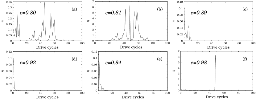
Figure 6: Figure showing the variation of synchronization error $\eta$ versus time in the coupled chaotic pendula for (a) $c=0.80$, (b) $c=0.81$, (c) $c=0.89$, (d) $c=0.92$, (e) $c=0.94$ and (f) $c=0.98$. Fluctuation in $\eta$ shows the possibility of having intermittent synchronization. In calculating $\eta$, tiny noise levels ($\approx 10^{-15}$) are included at each time step to avoid round off induced synchronization.

For the coupled chaotic pendula (9), as shown in Ref. baker the eigenvalues of the Jacobian matrix corresponding to the flow evaluated on the synchronization manifold take the form

$$\lambda_{1,2} = \frac{-1}{2Q}\left[1\pm\sqrt{1-2Q^{2}(1-c)\cos\theta_{\text{sm}}}\right],$$

$$\lambda_{3} = 0.$$ (11)

Here $\theta_{\text{sm}}$ corresponds to the angle coordinate on the synchronization manifold. On careful numerical observation, it has been shown by Baker, Blackburn and Smith baker that the term inside the square root sign varies chaotically about unity with an average value which is slightly less than one for a range of $c$ values. This implies that the largest eigenvalue is not always less than zero and hence the condition (i) is not obeyed uniformly.

Further, calculating the Lyapunov function which is the square of the magnitude of the vector describing the distance from the synchronization manifoldgauthier , the sufficient condition for permanent synchronization can be written asbaker

$$\dot{E}=\left(1-c-\cos\theta_{\text{sm}}\right)\theta^{*}\omega^{*}-Q^{-1}\omega^{*2}\leq 0,$$ (12)

where $\omega=\dot{\theta}$, $\theta^{*}=\theta_{m}-\theta_{s}$ and $\omega^{*}=\omega_{m}-\omega_{s}$. The time series of the above expression varies intermittently about zero with an average slightly less than zero for a range of $c$ values [$c\in(0.79,1.0)$] and hence the condition (ii) is also not obeyed for the coupled chaotic pendula. Thus, in the light of the above evidence, Baker, Blackburn and Smith baker ; baker2 conclude that intermittent synchronization can be a plausible behaviour in the coupled pendulum as the locking occurs intermittently. In order to verify this assertion, we have carried out an analysismuru1 by calculating the conditional Lyapunov exponents of system (9) in the parameter range $c\in(0.75,1.0)$. We find that there exists a range of $c$ values for which one can indeed have permanent synchronization, where Baker, Blackburn and Smithbaker have expected intermittent synchronization. In our calculations we have used the standard Wolf et al algorithmwolf and used $5000$ drive cycles for calculations after leaving out $5000$ drive cycles as transient.

Figure 5(a) shows the variation of CLE as a function of $c$ for the coupled pendula and it takes negative values for $0.796\leq c<1.0$ only. The CLE value for $c=0.79$ is $+0.00320$ ($\approx 10^{-3}$), for which synchronization can not occur and hence the observed intermittent synchronization (see Fig. 1 in Ref baker ) is a computer artifact. However, we find that for $c=0.932$, the CLE value becomes the lowest ($-0.06825$) and it is relatively a large negative value for which intermittent synchronization is absent as shown in Fig. 5(b). The absence of the intermittent synchronization has been verified upto $2\times 10^{6}$ drive cycles even with the addition of tiny noise levels showing that permanent synchronization does occur for this value of $c$. The same phenomenon persists over a range of $c$ values close to $0.932$. Figs. 6 show the variation of the synchronization error for various $c$ values. From the figures it is clear that one can indeed have intermittent synchronization for a range of $c$ values as noted by Baker, Blackburn and Smithbaker . For example, the system definitely exhibits intermittent synchronization for $c=0.80$, $0.81$ and $0.98$, where we find that in this range of $c$ values (that is, $c\leq 0.88$ or $c\geq 0.95$) the largest CLEs take values very close to zero (either positive or negative). But more interestingly we also find that there exists another range of $c$ values from $0.89$ to $0.94$ where one can have permanent synchronization. In calculating $\eta$ for Figs. 6(a)-(f), we have added a small amount of noise ($\approx 10^{-15}$) at each time step to avoid the effect of round off induced

Figure 7: Figure showing the variation of time of synchronization $t_{s}$ (in drive cycles) versus coupling strength for coupled chaotic pendula.

synchronization. We note that the CLEs are negative and the largest CLE is relatively away from zero in this range. Thus we note that the actual values of the CLEs, including the largest CLE, seem to distinguish between permanent and intermittent synchronization.

Next we calculate the time of synchronization ($t_{s}$), that is, the time taken by the system for which the synchronization error becomes zero. Fig. 7 depicts the variation of $t_{s}$ as a function of the coupling coefficient. It can be easily seen that the value of $t_{s}$ is very low for the range of $c$ values where the CLEs are large negative which corresponds to permanent synchronization. Similarly, the value of $t_{s}$ becomes high in the regions where the largest CLE has a value close to zero (either negative or positive) which corresponds to intermittent synchronization, as there exists large fluctuations in the finite time Lyapunov exponents here.

It is clear from the above analysis on the coupled chaotic pendula (9) that there exists intermittent synchronization for certain ranges of coupling strength values. However, permanent synchronization does occur for certain other range of $c$ values. In particular, we have pointed out that when the CLEs become very close to zero (either positive or negative) one can have intermittent synchronization while permanent synchronization does occur when the CLEs become large negative. Thus the CLEs play a crucial role in distinguishing between intermittent and permanent synchronization. In the following subsections we will examine the existence of similar intermittent synchronization in the coupled Duffing equations and coupled MLC circuits.

IV.2 Coupled Duffing oscillators

Now we consider the case of two coupled Duffing oscillators described by the following set of equations,

$$\ddot{x}_{m}+\alpha\dot{x}_{m}+\beta x_{m}^{3}=f\cos\omega t,$$ (13a)

$$\ddot{x}_{s}+\alpha\dot{x}_{s}+\beta x_{s}^{3}=f\cos\omega t+c(x_{s}-x_{m}),$$ (13b)

where $\alpha=0.1$, $\beta=1.0$, $f=10$ and $\omega=1.0$ and $c$ is the coupling strength. By setting $\dot{x}=y$, $z=\omega t$, one can rewrite the above equations as a set of first order ordinary differential equations of the form

$$\dot{x}_{m} = y_{m}$$

$$\dot{y}_{m} = -\alpha y_{m}-\beta x_{m}^{3}+f\cos z_{m}$$

$$\dot{z}_{m} = \omega$$ (14a)

$$\dot{x}_{s} = y_{s}$$

$$\dot{y}_{s} = -\alpha y_{s}-\beta x_{s}^{3}+f\cos z_{s}+c(x_{s}-x_{m})$$

$$\dot{z}_{s} = \omega$$ (14b)

First, we study the nature of synchronization in the above coupled Duffing equations by analysing the conditions (i) and (ii) of Sec. II as in the case of chaotic pendula

Figure 8: (a) Variation of the conditional Lyapunov exponent (CLE) as a function of $c$ and (b) synchronization error $\eta$ for coupled Duffing oscillators.

discussed above. Here the eigenvalues of the Jacobian matrix corresponding to the flow evaluated on the synchronization manifold can be explicitly written as

$$\lambda_{1,2}=\frac{-\alpha\pm\sqrt{\alpha^{2}+4(3\beta x_{\text{sm}}^{2}+c)}}{2\alpha},\;\;\;\;\lambda_{3}=0,$$ (15)

where $x_{\text{sm}}$ denotes the $x$-variable evaluated on the synchonization manifold. We found that the largest of eigenvalue oscillates chaotically about zero with an average value very close to

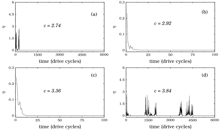
Figure 9: Figure showing the variation of synchronization error $\eta$ versus time in the coupled Duffing oscillators for (a) $c=2.74$, (b) $c=2.92$, (c) $c=3.36$ and (d) $c=3.84$ with the inclusion of tiny noise levels of the order of $10^{-15}$ at each integration step.

zero ($\approx\pm 10^{-3}$) for two ranges of $c\in(1.48,1.64)$ and $c\in(2.74,3.84)$. Thus the condition (i) is not uniformly obeyed. In addition, one can write the condition (ii) as

$$\dot{E}=(1-3\beta x_{\text{sm}}^{2}-c)x^{*}y^{*}-\alpha y^{*2}\leq 0,$$ (16)

with $x^{*}=x_{m}-x_{s}$ and $y^{*}=y_{m}-y_{s}$. On actual numerical simulation, it has been found that the time series of the above expression oscillates chaotically about zero with an average of the order of $\pm 10^{-3}$. This confirms that the condition (ii) is also not satisfied uniformly. Thus, the only way to

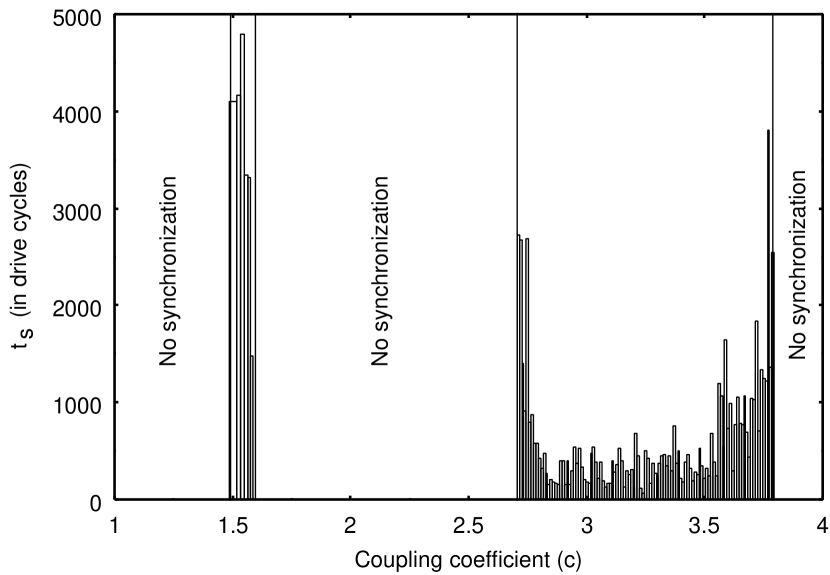
Figure 10: Figures showing the variation of time of synchronization $t_{s}$ versus $c$ in the coupled Duffing oscillators.

understand the nature of synchronization in Eqs. (14) is to analyse the CLEs. We have again calculated the largest CLE as a function of the coupling strength. Fig. 8 shows a plot of the largest CLE versus coupling strength ($c$). We find that the CLE takes small negative values close to zero ($\approx 10^{-3}$) for $c\in(1.48,1.64)$, where synchronization is essentially intermittent and numerical artifact does arise in this range. In addition, there exists another range of $c$ values, $2.74\leq c\leq 3.84$, where the CLEs are again negative (cf. Fig. 8(a)). We find that for $c=3.06$, the CLE takes the lowest value of $-0.05967$ (large negative value) for which persistent synchronization occurs and the intermittent synchronization is absent (cf. Fig. 8(b)). The variation of synchronization error for a range of selected $c$ values is depicted in Figs. 9(a)-(d). It can be noted from the figures that for $c=2.74$ and $3.84$ (Fig. 9(a) and (d)) the system can exhibit intermittent synchronization while for $c=2.92$ and $3.36$ (Fig. 9(b) and (c)) the system exhibits permanent synchronization. Here also tiny noise levels in all the variables were included at each integration step to ensure the absence of round off induced synchronization.

As in the case of coupled pendula, we have calculated the time of synchronization ($t_{s}$) by varying the coupling strength. Fig. 10 shows the variation of $t_{s}$ as a function of the coupling strength for this case. From the figure, it can be noted again that $t_{s}$ takes relatively low values for a region of $c$ values where the CLEs have large negative values which corresponds to permanent synchronization. Similarly, the values of $t_{s}$ becomes high in the regions where the largest CLE has a value close to zero or positive which corresponds to intermittent synchronization.

Figure 11: Figure showing (a) the variation of largest CLE as a function of the coupling coefficient $\varepsilon$ for the coupled MLC circuits and (b) blow up of a small region in (a) indicating the fluctuations of the largest CLE near zero.

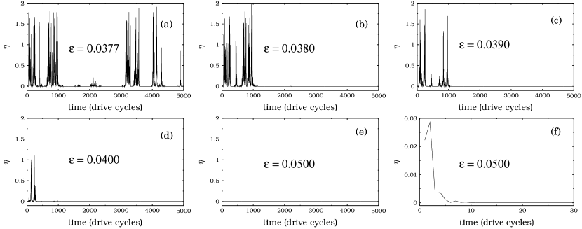
Figure 12: Figure showing the variation of synchronization error $\eta$ versus time in the coupled MLC circuits for (a) $\varepsilon=0.0377$, (b) $\varepsilon=0.0380$, (c) $\varepsilon=0.0390$, (d) $\varepsilon=0.0400$, (e) $\varepsilon=0.0500$ and (f) a small region in (e) with the inclusion of tiny noise levels at each integration step.

IV.3 Coupled MLC circuits

Finally we consider the case of the coupled Murali-Lakshmanan-Chua (MLC) circuits, represented by the following set of equationslakshman

$$\dot{x}_{m} = y_{m}-h(x_{m}),$$

$$\dot{y}_{m} = -\beta x_{m}+\sigma y_{m}+F\sin z_{m}$$

$$\dot{z}_{m} = \omega$$ (17a)

$$\dot{x}_{s} = y_{s}-h(x_{s})+\varepsilon(x_{m}-x_{s}),$$

$$\dot{y}_{s} = -\beta x_{s}+\sigma y_{s}+F\sin z_{s}$$

$$\dot{z}_{s} = \omega$$ (17b)

where $\varepsilon$ is the coupling strength and $h(x)=bx-0.5(a-b)(|x+1|-|x-1|)$. The uncoupled system of the above MLC circuits has been shown to exhibit chaos for the choice of parameter values $\beta=1$, $\sigma=1.015$, $a=-1.02$ and $b=-0.55$. We are interested to analyse the existence of intermittent synchronization in this case also.

First let us check the validity of the conditions (i) and (ii). In this case, the eigenvalues of the Jacobian matrix of the flow evaluated on the synchronization manifold can be written as

$$\lambda_{1,2} = -\frac{1}{2}\left[h^{\prime}(x_{\text{sm}})+\beta-\varepsilon\right]$$

$$\pm\frac{1}{2}\sqrt{\left[h^{\prime}(x_{\text{sm}})+\beta-\varepsilon\right]^{2}-4[(h^{\prime}-\varepsilon)\beta+\sigma]},$$

$$\lambda_{3} = 0.$$ (18)

Here $h^{\prime}(x_{\text{sm}})$ corresponds to the derivative of $h(x)$ with respect to $x$ variable evaluated on the synchronization manifold. From numerical analysis, we have found that the largest of the above eigenvalues oscillates chaotically about zero with an average slightly less than zero for a range of $\varepsilon\in(0.036,0.04)$ and thus the condition (i) is not uniformly obeyed. On the other hand, the condition (ii) for the coupled MLC circuits can be written as

$$\dot{E}=\left[\varepsilon-h^{\prime}(x_{\text{sm}})\right]x^{*2}-\beta y^{*2}+(1-\sigma)x^{*}y^{*}\leq 0,$$ (19)

with $x^{*}=x_{m}-x_{s}$ and $y^{*}=y_{m}-y_{s}$. Again by numerical analysis, we find that the above inequality is not uniformly obeyed and hence the condition (ii) is not satisfied. However, the coupled system (17) has been shown to exhibit perfect synchronizationlakshman . In order to analyse this we have evaluated the CLEs as in the case of chaotic pendula and Duffing oscillators.

The variation of the CLEs as a function of the coupling strength ($\varepsilon$) is shown in Fig. 11. The largest CLE changes its sign from positive to negative values at $\varepsilon=0.0377$ and it is slightly less than zero over the range $0.0377<\varepsilon\lesssim 0.04$. In this range the synchronization completely depends on the choice of initial conditions and the computer precision used. This implies that the observed synchronization is essentially due to the finite computational precision and accordingly locking ($\eta=0$) occurs after relatively long time, leading to an intermittent synchronization in this range of coupling strength.

We have also calculated the synchronization error ($\eta$) for various values of coupling strength as a function of time as in the case of previous systems and the results are depicted in Fig. 12. From Figs. 12(a)-(d), it is evident that one can have intermittent synchronization for $\varepsilon=0.0377$, $0.0380$, $0.0390$ and $0.04$. Fig. 12(e) and Fig. 12(f) indicates the presence of permanent synchronization for $\varepsilon=0.05$ where the sharp and quick fall off in the synchronization error towards zero occurs (see Fig. 12(f)).

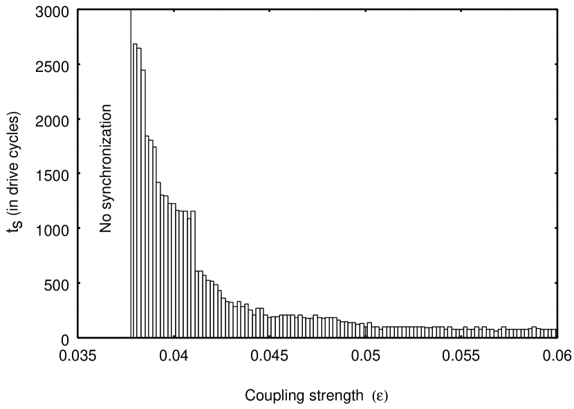
Figure 13: Figure showing the variation of time of synchronization $t_{s}$ versus coupling strength $\varepsilon$ for coupled MLC circuits.

Fig. 13 shows the variation of time of synchronization ($t_{s}$) as a function of the coupling strength ($\varepsilon$). As in the case of coupled pendula and Duffing oscillators, $t_{s}$ takes relatively low values for the range of $\varepsilon$ values where the CLEs take large negative values corresponding to permanent synchronization. However, the values of $t_{s}$ becomes high in the regions where the largest CLE has a value close to zero or positive which corresponds to intermittent synchronization. Thus one can conclude that permanent synchronization in coupled MLC circuits (17) occur for $\varepsilon>0.04$.

V Summary and conclusions

By considering typical examples of coupled oscillator models, we have discussed the quality of synchronization using various analytical and numerical tests. It has been noted that one can have an intermittent as well as permanent synchronization in the coupled oscillator systems depending on the choice of coupling strength. We have pointed out that the Conditional Lyapunov Exponents (CLEs) can be used to distinguish between the intermittent and permanent synchronization when the other criteria for asymptotic stability are not uniformly obeyed. Particularly, we find that intermittent synchronization can occur when CLEs are very small positive or negative values close to zero while persistent synchronization occurs when CLEs take sufficiently large negative values. This fact is further supported by the relative time taken for the system to approach the synchronization manifold.

The present work is mainly concerned with the qualitative analysis of chaos synchronization in unidirectionally coupled systems based on conditional Lyapunov exponents. In order to understand the entire dynamics one has to analyse the nature of the attractors that exist in the coupled system and their bifurcations. It is obvious that we have not made any quantitative analysis on how small or large be the magnitude of the largest conditional Lyapunov exponent in distinguishing the intermittent and permanent synchronizations. Work is in progress along these directions.

- (1) R. He and P. G. Vaidya, Phys. Rev. E 57, 1532 (1998).
- (2) L. M. Pecora and T. L. Corroll, Phys. Rev. Lett. 64, 821 (1990).
- (3) L. M. Pecora and T. L. Corroll, Phys. Rev. A 59, 2374 (1991).
- (4) J. W. Shuai, K. W. Wong, and L. M. Cheng, Phys. Rev. E 59, 2272 (1997).
- (5) J. Güémez, C. Marín, and M. A. Matías, Phys. Rev. E 55, 124 (1997).
- (6) J. M. Gutiérrez and A. Iglesias, Phys. Lett. A 239, 174 (1998).
- (7) G. L. Baker, J. A. Blackburn, and H. J. T. Smith, Phys. Rev. Lett. 81, 554 (1998).
- (8) G. L. Baker, J. A. Blackburn, and H. J. T. Smith, Phys. Lett. A 252, 191 (1999).
- (9) C. Zhou and C.-H. Lai, Phys. Rev. E 58, 5188 (1998).
- (10) M. Lakshmanan and K. Murali, Chaos in Nonlinear Oscillators: Controlling and Synchronization (World Scientific, Singapore, 1996).
- (11) K. Murali and M. Lakshmanan, Phys. Rev. E 48, R1624 (1993).
- (12) H. Fujisaka and T. Yamada, Prog. Theor. Phys. 69, 32 (1983).
- (13) H. Fujisaka and T. Yamada, Prog. Theor. Phys. 70, 1240 (1983).
- (14) R. He and P. G. Vaidya, Phys. Rev. A 46, 7387 (1992).
- (15) D. J. Gauthier and J. C. Bienfang, Phys. Rev. Lett. 77, 1751 (1996).
- (16) A. Wolf, J. B. Swift, H. L. Swinney, and J. A. Vastano, Physica D 77, 1751 (1996).
- (17) P. Muruganandam, S. Parthasarathy, and M. Lakshmanan, Phys. Rev. Lett. 83, 1259 (1999).
- (18) P. Muruganandam, Spatiotemporal Dynamics of Certain Discrete and Continuous Nonlinear Systems, Ph.D. thesis, Bharathidasan University (1999).