Classical dynamics on graphs

Abstract

We consider the classical evolution of a particle on a graph by using a time-continuous Frobenius-Perron operator which generalizes previous propositions. In this way, the relaxation rates as well as the chaotic properties can be defined for the time-continuous classical dynamics on graphs. These properties are given as the zeros of some periodic-orbit zeta functions. We consider in detail the case of infinite periodic graphs where the particle undergoes a diffusion process. The infinite spatial extension is taken into account by Fourier transforms which decompose the observables and probability densities into sectors corresponding to different values of the wave number. The hydrodynamic modes of diffusion are studied by an eigenvalue problem of a Frobenius-Perron operator corresponding to a given sector. The diffusion coefficient is obtained from the hydrodynamic modes of diffusion and has the Green-Kubo form. Moreover, we study finite but large open graphs which converge to the infinite periodic graph when their size goes to infinity. The lifetime of the particle on the open graph is shown to correspond to the lifetime of a system which undergoes a diffusion process before it escapes. PACS numbers:

02.50.-r (Probability theory, stochastic processes, and statistics);

03.65.Sq (Semiclassical theories and applications);

05.60.Cd (Classical transport);

45.05.+x (General theory of classical mechanics of discrete systems).

1 Introduction

The study of classical dynamics on graphs is motivated by the recent discovery that quantum graphs have similar spectral statistics of energy levels as the classically chaotic quantum systems [1, 2]. Since this pioneering work by Kottos and Smilansky, several studies have been devoted to the spectral properties of quantum graphs [3, 4, 5]. However, the classical dynamics, which is of great importance for the understanding of the short-wavelength quantum properties, has not yet been considered in detail. In Refs. [1, 2], a classical dynamics has been considered in which the particles are supposed to move on the graph with a discrete and isochronous (topological) time, ignoring the different lengths of the bonds composing the graph.

The purpose of the present paper is to develop the theory of the classical dynamics on graphs by considering the motion of particles in real time. This generalization is important if we want to compare the classical and quantum quantities, especially, with regard to the time-dependent properties in open or spatially extended graphs. A real-time classical dynamics on graphs should allow us to define kinetic and transport properties such as the classical escape rates and the diffusion coefficients, as well as the characteristic quantities of chaos such as the Kolmogorov-Sinai (KS) and the topological entropies per unit time.

An important question concerns the nature of the classical dynamics on a graph. A graph is a network of bonds on which the classical particle has a one-dimensional uniform motion at constant energy. The bonds are interconnected at vertices where several bonds meet. The number of bonds connected with a vertex is called the valence of the vertex. A quantum mechanics has been defined on such graphs by considering a wavefunction extending on all the bonds [1, 2]. This wavefunction has been supposed to obey the one-dimensional Schrödinger equation on each bond. The Schrödinger equation is supplemented by boundary conditions at the vertices. The boundary conditions at a vertex determine the quantum amplitudes of the outgoing waves in terms of the amplitudes of the ingoing waves and, thus, the transmission and reflection amplitudes of that particular vertex.

In the classical limit, the Schrödinger equation leads to Hamilton’s classical equations for the one-dimensional motion of a particle on each bond. When a vertex is reached, the square moduli of the quantum amplitudes give the probabilities that the particle be reflected back to the ingoing bond or be transmitted to one of the other bonds connected with the vertex. In the classical limit of arbitrarily short wavelengths, the transmission and reflection probabilities do not reduce to the trivial ones (i.e., to zero and one) for typical graphs. Accordingly, the limiting classical dynamics on graphs is in general a combination of the uniform motion of the particle on the bonds with random transitions at the vertices. This dynamical randomness which naturally appears in the classical limit is at the origin of a splitting of the classical trajectory into a tree of trajectories. This feature is not new and has already been observed in several processes such as the ray splitting in billiards divided by a potential step [6] or the scattering on a wedge [7]. We should emphasize that this dynamical randomness manifests itself only on subsets with a dimension lower than the phase space dimension and not in the bulk of phase space, so that the classical graphs share many properties of the deterministic chaotic systems, as we shall see below.

The dynamical randomness of the classical dynamics on graphs requires a Liouvillian approach to describe the time evolution of the probability density to find the particle somewhere on the graph. Accordingly, one of our first goals below will be to derive the Frobenius-Perron operator as well as the associated master equation for the graphs. This operator is introduced by noticing that the classical dynamics on a graph is equivalent to a random suspended flow determined by the lengths of the bonds, the velocity of the particle, and the transition probabilities.

A consequence of the dynamical randomness is the relaxation of the probability density toward the equilibrium density in typical closed graphs, or to zero in open graphs or in graphs of infinite extension. This relaxation can be characterized by the decay rates which are given by solving the eigenvalue problem of the Frobenius-Perron operator. The characteristic determinant of the Frobenius-Perron operator defines a classical zeta function and its zeros – also called the Pollicott-Ruelle resonances – give the decay rates. The leading decay rate is the so-called escape rate. The Pollicott-Ruelle resonances have a particularly important role to play because they control the decay or relaxation and they also manifest themselves in the quantum scattering properties of open systems, as revealed by a recent experiment by Sridhar and coworkers [8]. The decay rates are time-dependent properties so that they require to consider the continuous-time classical dynamics to be defined.

Besides, we define a continuous-time “topological pressure” function from which the different chaotic properties of the classical dynamics on graphs can be deduced. This function allows us to define the KS and topological entropies per unit time, as well as an effective positive Lyapunov exponent for the graph.

We shall also show how diffusion can be studied on spatially periodic graphs thanks to our Frobenius-Perron operator and its decay rates. Here, we consider graphs that are constructed by the repetition of a unit cell. When the cell is repeated an infinite number of times we form a periodic graph. Such spatially extended periodic systems are interesting for the study of transport properties. In fact at the classical level it has been shown in several works that relationships exist between the chaotic dynamics and the normal transport properties such as diffusion [9] and the thermal conductivity [10], which have been studied in the periodic Lorentz gas. In the present paper, we obtain the continuous-time diffusion properties for the spatially periodic graphs. Moreover, we also study the escape rate in large but finite open graphs and we show that this rate is related, on the one hand, to the diffusion coefficient and, on the other hand, to the effective Lyapunov exponent and the KS entropy per unit time.

The plan of the paper is the following. Sec. 2 contains a general introduction to the graphs and their classical dynamics. In Subsec. 2.2, we introduce the evolution using the aforementioned random suspended flow and, therefore, we can follow the approach developed in Ref. [9] for the study of relaxation and chaotic properties at the level of the Liouvillian dynamics which is developed in Sec. 3. The Frobenius-Perron operator is derived in Subsec. 3.1. In Subsec. 3.2, we present an alternative derivation of the Frobenius-Perron operator and its eigenvalues and eigenstates, which is based on a master-equation approach, familiar in the context of stochastic processes. Both approaches are shown to be equivalent. In Sec. 4, we study the relaxation and ergodic properties of the graphs in terms of the classical zeta function and its Pollicott-Ruelle resonances. In Sec. 5, the large-deviation formalism is introduced which allows us to characterize the chaotic properties of these systems. In Sec. 6, the theory is applied to classical scattering on open graphs. The case of infinite periodic graphs is considered in Sec. 7, where we obtain the diffusion coefficient and we show that it can be written in the form of a Green-Kubo formula. In Sec. 8, we consider finite open graphs of the scattering type, where the particle escape to infinity, and we show how the diffusion coefficient can be related to the escape rate and the chaotic properties. The case of infinite disordered graphs is considered in Sec. 9. Conclusions are drawn in Sec. 10.

2 The graphs and their classical dynamics

2.1 Definition of the graphs

Now, let us introduce graphs as geometrical objects where a particle moves. Graphs are $V$ vertices connected by $B$ bonds. Each bond $b$ connects two vertices, $i$ and $j$. We can assign an orientation to each bond and define “oriented or directed bonds”. Here one fixes the direction of the bond $[i,j]$ and call $b=(i,j)$ the bond oriented from $i$ to $j$. The same bond but oriented from $j$ to $i$ is denoted $\hat{b}=(j,i)$. We notice that $\hat{\hat{b}}=b$. A graph with $B$ bonds has $2B$ directed bonds. The valence $\nu_{i}$ of a vertex is the number of bonds that meet at the vertex $i$.

Metric information is introduced by assigning a length $l_{b}$ to each bond $b$. In order to define the position of a particle on the graph, we introduce a coordinate $x_{b}$ on each bond $b=[i,j]$. We can assign either the coordinate $x_{(i,j)}$ or $x_{(j,i)}$. The first one is defined such that $x_{(i,j)}=0$ at $i$ and $x_{(i,j)}=l_{b}$ at $j$, whereas $x_{(j,i)}=0$ at $j$ and $x_{(j,i)}=l_{b}$ at $i$. Once the orientation is given, the position of a particle on the graph is determined by the coordinate $x_{b}$ where $0\leq x_{b}\leq l_{b}$. The index $b$ identifies the bond and the value of $x_{b}$ the position on this bond.

For some purposes, it is convenient to consider $b$ and $\hat{b}$ as different bonds within the formalism. Of course, the physical quantities defined on each of them must satisfy some consistency relations. In particular, we should have that $l_{\hat{b}}=l_{b}$ and $x_{\hat{b}}=l_{b}-x_{b}$.

A particle on a graph moves freely as long as it is on a bond. The vertices are singular points, and it is not possible to write down the analogue of Newton’s equations at the vertices. Instead we have to introduce transition probabilities from bond to bond. These transition probabilities introduce a dynamical randomness which is coming from the quantum dynamics in the classical limit. In this sense, the classical dynamics on graphs turns out to be intrinsically random.

The reflection and transmission (transition) probabilities are determined by the quantum dynamics on the graph. This latter introduces the probability amplitudes $T_{bb^{\prime}}$ for a transition from the bond $b^{\prime}$ to the bond $b$. We shall show in a separate paper [11] that the random classical dynamics defined in the present paper, with the transition probabilities defined by $P_{bb^{\prime}}=|T_{bb^{\prime}}|^{2}$ is, indeed, the classical limit of the quantum dynamics on graphs. For example, we may consider a quantum graph with transition amplitudes of the form

$$T_{bb^{\prime}}=C_{bb^{\prime}}\left(\frac{2}{\nu_{bb^{\prime}}}-\delta_{\hat{b^{\prime}}b^{\prime}}\right)$$ (1)

where $C_{bb^{\prime}}$ is 1 if the bond $b^{\prime}$ is connected with the bond $b$ and zero otherwise and $\nu_{bb^{\prime}}$ is the valence of the vertex that connects $b^{\prime}$ with $b$. Such probability amplitudes are obtained once we impose the continuity of the wave function and the current conservation at each vertex.

For the classical dynamics on graphs, the energy of the particle is conserved during the free motion in the bonds and also in the transition to other bonds. Accordingly, we consider the surface of constant energy in the phase space determined by the coordinate of the particle, that is $x_{b}$ which specifies a bond and the position with respect to a vertex. The momentum is simply given by the direction in which the particle moves on the bond. The modulus of the momentum is fixed by the energy. We see that position and direction can be combined together if we speak about position in a given directed bond. In this way our phase space are the points of the directed bonds. The equation of motion is thus

$$\frac{dx}{dt}=v=\sqrt{2E/M}\ ,\qquad\hbox{for}\qquad 0<x=x_{b}<l_{b}\ ,$$ (2)

where $v$ is the velocity in absolute value, $E$ the energy, and $M$ the mass of the particle. When the particle reaches the end $x_{b^{\prime}}=l_{b^{\prime}}$ of the bond $b^{\prime}$ a transition can bring it at the beginning $x_{b}=0$ of the bond $b$. According to the above discussion, we assume moreover that this transition from the bond $b^{\prime}$ to the bond $b$ has the probability $P_{bb^{\prime}}$ to occur:

$$\mbox{transition}\quad b^{\prime}\to b\quad\mbox{with probability}\quad P_{bb^{\prime}}$$ (3)

By the conservation of the total probability, the transition probabilities must satisfy

$$\sum_{b}P_{bb^{\prime}}=1$$ (4)

which means that the vector $\{1,1,\ldots,1\}$ is always a left eigenvector with eigenvalue $1$ for the transition matrix $\mathsf{P}=\{P_{bb^{\prime}}\}_{b,b^{\prime}=1}^{2B}$.

We may assume that the system has the property of microscopic reversibility (i.e., of detailed balancing) according to which the probability of the transition $b^{\prime}\to b$ is equal to the probability of the time-reversed transition $\hat{b}\to\hat{b^{\prime}}$: $P_{bb^{\prime}}=P_{\hat{b^{\prime}}\hat{b}}$, as expected for instance in absence of a magnetic field. As a consequence of detailed balancing, the matrix $\mathsf{P}$ is a bi-stochastic matrix, i.e., it satisfies $\sum_{b}P_{bb^{\prime}}=\sum_{b^{\prime}}P_{bb^{\prime}}=1$, whereupon the vector $\{1,1,\ldots,1\}$ is both a right and left eigenvector of $\mathsf{P}$ with eigenvalue $1$. This is the case for a finite graph with transition probabilities $P_{bb^{\prime}}=|T_{bb^{\prime}}|^{2}$ given by the amplitudes (1).

2.2 The classical dynamics on graphs as a random suspended flow

The description given above is analogous to the dynamics of a so-called suspended flow [9]. In fact, we can consider the set of points $\left\{x_{b}=0,\ \forall b\right\}$, i.e., the set of all vertices, as a surface of section. We attach to each of these points a segment (here the directed bond) characterized by a coordinate $0<x<l_{b}$. When the trajectory reaches the point $x=l_{b}$ it performs another passage through the surface. Thus the flow is suspended over the Poincaré surface of section made of the vertices in the phase space of the directed bonds.

For convenience, instead of the previous notation $x_{b}$, the position (in phase space) will be referred to as the pair $\left[b,x\right]$ where $b$ indicates the directed bond and $x$ is the position on this bond, i.e., $0<x<l_{b}$.

A realization of the random process on the graph (i.e., a trajectory) can be identified with the sequence of traversed bonds $\cdots b_{-2}b_{-1}b_{0}b_{1}b_{2}\cdots$ (which is enough to determine the evolution on the surface of section). The probability of such a trajectory is given by $\cdots P_{b_{2}b_{1}}P_{b_{1}b_{0}}P_{b_{0}b_{-1}}P_{b_{-1}b_{-2}}\cdots$.

An initial condition $[b_{0},x]$ of this trajectory is denoted by the dotted bi-infinite sequence $\cdots b_{-2}b_{-1}\cdot b_{0}b_{1}b_{2}\cdots$ together with the position $0\leq x<l_{b_{0}}$. For a given trajectory, we divide the time axis in intervals of duration $\frac{l_{b_{n}}}{v}$ extending from

$$\frac{l_{b_{0}}-x}{v}+\frac{l_{b_{1}}}{v}+\cdots+\frac{l_{b_{n-2}}}{v}+\frac{l_{b_{n-1}}}{v}\text{\quad to\quad}\frac{l_{b_{0}}-x}{v}+\frac{l_{b_{1}}}{v}+\cdots+\frac{l_{b_{n-2}}}{v}+\frac{l_{b_{n-1}}}{v}+\frac{l_{b_{n}}}{v}$$

where $v$ is the velocity of the particle which travels freely in the bonds. At each vertex, the particle changes its direction but keeps constant its kinetic energy.

For a trajectory $p$ that, at time $t=0$, is at the position $[b_{0},x]$ we define the forward evolution operator $\Phi_{p}^{t}$ with $t>0$ by

$$\Phi_{p}^{t}\left[b_{0},x\right]=\left[b_{0},vt+x\right]\qquad\text{if }\qquad 0<x+vt<l_{b_{0}}$$ (5)

i.e., the evolution is the one of a free particle as long as the particle stays in the bond $b_{0}$, and

$$\Phi_{p}^{t}\left[b_{0},x\right]=\left[b_{n},x+vt-l_{b_{n-1}}-l_{b_{n-2}}-\cdots-l_{b_{0}}\right]\\ \text{if\quad}0<x+vt-l_{b_{n-1}}-l_{b_{n-2}}-\cdots-l_{b_{0}}<l_{b_{n}}$$ (6)

which follows from the fact that, for the given trajectory $p$, the bond and the position where the particle stands at a given time is fixed by the lengths traversed at previous times and by the constant velocity $v$. Analogously, we also introduce a backward evolution for $t<0$:

$$\Phi_{p}^{-|t|}\left[b_{0},x\right]=\left[b_{0},x-v|t|\right]\qquad\text{if }\qquad 0<x-v|t|<l_{b_{0}}$$

and

$$\Phi_{p}^{-|t|}\left[b_{0},x\right]=\left[b_{-n},x-v|t|+l_{b_{-n}}+l_{b_{-n+1}}+\cdots+l_{b_{-1}}\right]\\ \text{if\quad}0<x-v|t|+l_{b_{-n}}+l_{b_{-n+1}}+\cdots+l_{b_{-1}}<l_{b_{-n}}$$

3 The Liouvillian description

3.1 The Frobenius-Perron operator

On the graph, we want to study the time evolution of the probability density $\rho\left(\left[b,x\right],t\right)$. This density determines the probability $\rho\left(\left[b,x\right],t\right)dx$ of finding the particle in the bond $b$ with position in $[x,x+dx]$ at time $t$.

For a general Markov process, the time evolution of the probability density is ruled by the Chapman-Kolmogorov equation

$$\rho(\xi,t)=\int d\xi_{0}\,{\cal P}\left(\xi,t|\xi_{0},t_{0}\right)\rho(\xi_{0},t_{0})$$ (7)

where ${\cal P}\left(\xi,t|\xi_{0},t_{0}\right)$ is the conditional probability density that the particle be in the state $\xi$ at time $t$ given that it was in the state $\xi_{0}$ at the initial time $t_{0}$. This conditional probability density defines the integral kernel of the time-evolution operator, which is linear. The conditional probability density can be expressed as a sum (or integral) over all the paths joining the initial state to the final one within the given lapse of time.

In the case of graphs, each state is given by an directed bond and a position on this bond: $\xi=[b,x]$. A path or trajectory is a bi-infinite sequence of directed bonds as described in the preceding section. As soon as the path or trajectory $p$ is known, the sequence of visited bonds is fixed so that the motion is determined to be the time translation at velocity $v$ given by Eqs. (5)-(6). In this case, the conditional probability density of finding the particle in position $[b,x]$ at time $t$ given it was in $[b_{0},x_{0}]$ at the initial time $t_{0}=0$ is given by a kind of Dirac delta density $\delta\left(\left[b,x\right]-\Phi_{p}^{t}\left[b_{0},x_{0}\right]\right)$. Along the path $p$, the particle meets several successive vertices where the conditional probability density is expressed in terms of the conditional probability to reach the final bond $b=b_{n}$ within the time $t$, given the initial condition $[b_{0},x_{0}]$:

$$P_{p}(t,[b_{0},x_{0}])\equiv({\mathsf{P}}^{n})_{bb_{0}}=P_{bb_{n-1}}P_{b_{n-1}b_{n-2}}\cdots P_{b_{2}b_{1}}P_{b_{1}b_{0}}$$ (8)

We notice that the integer $n$ is fixed by the trajectory $p$, the initial condition $[b_{0},x_{0}]$, and the elapsed time $t$. The number of the path probabilities (8) which are non-vanishing is always finite if there is no sequence of lengths accumulating to zero for the graph under study.

For a graph, the kernel of the evolution operator is thus given by

$${\cal P}\left(\left[b,x\right],t|\left[b_{0},x_{0}\right],0\right)=\sum_{\{p\}}P_{p}(t,[b_{0},x_{0}])\;\delta\left(\left[b,x\right]-\Phi_{p}^{t}\left[b_{0},x_{0}\right]\right),$$ (9)

where the sum is performed over a finite number of paths. By analogy with Eq. (7) the density is given by

$$\rho\left(\left[b,x\right],t\right)=\sum_{b_{0}}\int_{0}^{l_{b_{0}}}dx_{0}\left(\sum_{\{p\}}P_{p}(t,[b_{0},x_{0}])\;\delta\left(\left[b,x\right]-\Phi_{p}^{t}\left[b_{0},x_{0}\right]\right)\right)\rho\left(\left[b_{0},x_{0}\right],0\right)$$

and integrating the Dirac delta density we finally get

$$\rho\left(\left[b,x\right],t\right)=\sum_{\{p\}}P_{p}(t,\Phi_{p}^{-t}\left[b,x\right])\ \rho\left(\Phi_{p}^{-t}\left[b,x\right],0\right).$$ (10)

where the sum is over all the trajectories that go backward in time from the current point $\left[b,x\right]$.

In this way, we have defined the Frobenius-Perron operator $\hat{P}^{t}$ as

$$\hat{P}^{t}\,F\left[b,x\right]=\sum_{\{p\}}P_{p}(t,\Phi_{p}^{-t}\left[b,x\right])\ F\left(\Phi_{p}^{-t}\left[b,x\right]\right)$$ (11)

where $\left\{F[b,x]\right\}$ is a vector of $2B$ functions defined on the directed bonds.

We now turn to the determination of the spectrum of the Frobenius-Perron operator. With this aim, we take the Laplace transform of the Frobenius-Perron operator given by Eq. (11):

$$\int_{0}^{\infty}\mbox{e}^{-st}\hat{P}^{t}\,F\left[b,x\right]dt=\int_{0}^{\infty}dt\,\mbox{e}^{-st}\sum_{\{p\}}P_{p}(t,\Phi_{p}^{-t}\left[b,x\right])\ F\left(\Phi_{p}^{-t}\left[b,x\right]\right)$$

In order to evaluate the Laplace transform, we have to decompose the sum over the paths $\{p\}$ into the different classes of terms corresponding to paths in which $n=0,1,2,...$ bonds are visited during the time $t$. This decomposition leads to

$$\sum_{\{p\}}\int_{0}^{\infty}\mbox{e}^{-st}P_{p}\ F\left(\Phi_{p}^{-t}\left[b,x\right]\right)dt=\int_{0}^{\frac{x}{v}}\mbox{e}^{-st}F\left[b,x-vt\right]dt\\ +\sum_{n=1}^{\infty}\sum_{\{p^{-n}\}}\int_{\frac{x}{v}+\Sigma_{i=1}^{n-1}\frac{l_{b_{-i}}}{v}}^{\frac{x}{v}+\Sigma_{i=1}^{n}\frac{l_{b_{-i}}}{v}}\,\mbox{e}^{-st}\,P_{p^{-n}}\,F\left[b_{-n},x-vt+\sum_{i=1}^{n}l_{b_{-i}}\right]dt$$

with $P_{p^{-n}}=P_{bb_{-1}}P_{b_{-1}b_{-2}}\cdots P_{b_{-n+1}b_{-n}}$ the probability of a path $p^{-n}$ and $\sum_{\{p^{-n}\}}$ the sum over these trajectories. A change of variable transforms the previous equation in the following

$$\sum_{\{p\}}\int_{0}^{\infty}\mbox{e}^{-st}P_{p}\;F\left(\Phi_{p}^{-t}\left[b,x\right]\right)=\frac{1}{v}\;\mbox{e}^{-s\frac{x}{v}}\left\{\int_{0}^{x}\mbox{e}^{s\frac{x^{\prime}}{v}}F\left[b,x^{\prime}\right]dx^{\prime}\right.\\ \left.+\sum_{n=1}^{\infty}\sum_{\{p^{-n}\}}\left(\prod_{i=1}^{n}Q_{b_{-i+1}b_{-i}}\right)\int_{0}^{l_{b_{-n}}}\mbox{e}^{-s\frac{x^{\prime}}{v}}F\left[b_{-n},x^{\prime}\right]dx^{\prime}\right\}$$ (12)

where we introduced the quantity

$$Q_{bb^{\prime}}(s)=P_{bb^{\prime}}\;\mbox{e}^{-s\frac{l_{b^{\prime}}}{v}}$$ (13)

and here we identify $b_{0}$ with $b$. Now we have to perform the sum over all the realizations in the right-hand side of Eq. (12). This is a sum over all the trajectories $b_{-1}b_{-2}\cdots b_{-n+1}b_{-n}$ which leads to the formation of the matrix ${\mathsf{Q}}^{n}$, i.e., $\mathsf{Q}$ raised to the power $n$. Accordingly, we get

$$\int_{0}^{\infty}\mbox{e}^{-st}\hat{P}^{t}\,F\left[b,x\right]dt=\frac{1}{v}\;\mbox{e}^{-sx/v}\left\{\int_{0}^{x}\mbox{e}^{s\frac{x^{\prime}}{v}}F\left[b,x^{\prime}\right]dx^{\prime}\right.\\ \left.+\sum_{n=1}^{\infty}\sum_{b_{-n}}\left({\mathsf{Q}}^{n}\right)_{bb_{-n}}\int_{0}^{l_{b_{-n}}}\mbox{e}^{s\frac{x^{\prime}}{v}}F\left[b_{-n},x^{\prime}\right]dx^{\prime}\right\}.$$ (14)

We define the vector ${\mathbf{f}}(s)=\{f_{1}(s),...,f_{2B}(s)\}$ with the components of this vector given by the functions

$$f_{b}(s)=\int_{0}^{l_{b}}\mbox{e}^{s\frac{x^{\prime}}{v}}F\left[b,x^{\prime}\right]dx^{\prime}$$ (15)

The matrix ${\mathsf{Q}}(s)$ acts on these vectors ${\mathbf{f}}(s)$ through the relation

$$\left({\mathsf{Q}}\cdot{\mathbf{f}}\right)_{b}(s)=\sum_{b^{\prime}}Q_{bb^{\prime}}(s)f_{b^{\prime}}(s).$$ (16)

This matrix can be interpreted as the Frobenius-Perron operator of the evolution reduced to the surface of section [9]. This matrix depends on the Laplace variable $s$ which will give the relaxation rate of the system. With these definitions, we can write

$$\sum_{n=1}^{\infty}\sum_{b_{-n}}\left({\mathsf{Q}}^{n}\right)_{bb_{-n}}\int_{0}^{l_{b_{-n}}}\mbox{e}^{s\frac{x^{\prime}}{v}}F\left[b_{-n},x^{\prime}\right]dx^{\prime}=\sum_{n=1}^{\infty}\left({\mathsf{Q}}^{n}\cdot{\mathbf{f}}\right)_{b}(s)=\left(\frac{\mathsf{Q}}{{\mathsf{I}}-{\mathsf{Q}}}\cdot{\mathbf{f}}\right)_{b}(s)$$

where we used the relation $\sum_{n=1}^{\infty}{\mathsf{Q}}^{n}=\frac{{\mathsf{Q}}}{{\mathsf{I}}-{\mathsf{Q}}}$. As a consequence, Eq. (14) becomes

$$\int_{0}^{\infty}\mbox{e}^{-st}\hat{P}^{t}\,F\left[b,x\right]dt=\frac{1}{v}\;\mbox{e}^{-sx/v}\left\{\int_{0}^{x}\mbox{e}^{s\frac{x^{\prime}}{v}}F\left[b,x^{\prime}\right]dx^{\prime}+\left(\frac{\mathsf{Q}}{{\mathsf{I}}-{\mathsf{Q}}}\cdot{\mathbf{f}}\right)_{b}(s)\right\}.$$ (17)

We are now at a few steps from determining the eigenvalues (and eigenvectors) of $\hat{P}^{t}$. This is done by first studying the solutions of

$${\mathsf{Q}}(s)\cdot{\mathbf{f}}(s)={\mathbf{f}}(s).$$

These solutions exist only if $s$ belongs to the (complex) set $\left\{s_{j}\right\}$ of solutions of the following characteristic determinant

$$\det\left[{\mathsf{I}}-{\mathsf{Q}}(s)\right]=0$$ (18)

We denote these particular vectors by $\boldsymbol{\chi}_{j}$ and their components by $\chi_{j}[b]$ with $b=1,...,2B$, whereupon

$${\mathsf{Q}}(s_{j})\cdot\boldsymbol{\chi}_{j}=\boldsymbol{\chi}_{j}.$$ (19)

The left vector which is adjoint to the right vector $\boldsymbol{\chi}_{j}$ is given by

$${\mathsf{Q}}(s_{j})^{\dagger}\cdot\tilde{\boldsymbol{\chi}}_{j}=\tilde{\boldsymbol{\chi}}_{j}.$$ (20)

The relation to the eigenvalue problem of the flow is established as follows. Suppose that $\Psi_{j}\left[b,x\right]$ is an eigenstate of $\hat{P}^{t}$ with eigenvalue $\mbox{e}^{s_{j}t}$ [for the moment $s_{j}$ is not determined but we call it this way because it will turn out to be one of the solutions of Eq. (18)], i.e.,

$$\hat{P}^{t}\,\Psi_{j}\left[b,x\right]=\mbox{e}^{s_{j}t}\Psi_{j}\left[b,x\right]$$ (21)

with ${\mathrm{R}e}\,s_{j}\leq 0$ because the density is not expected to increase with the time. For the forward semigroup, the zeros of Eq. (18) are expected in the region ${\mathrm{R}e}\,s_{j}\leq 0$.

Taking the Laplace transform of Eq. (21), we get

$$\int_{0}^{\infty}dt\,\mbox{e}^{-st}\,\hat{P}^{t}\,\Psi_{j}\left[b,x\right]=\int_{0}^{\infty}dt\,\mbox{e}^{(s_{j}-s)t}\Psi_{j}\left[b,x\right]=\frac{\Psi_{j}\left[b,x\right]}{s-s_{j}}$$

If we introduce the vector $\boldsymbol{\Upsilon}(s)=\{\Upsilon_{1}(s),...,\Upsilon_{2B}(s)\}$ defined by the components

$$\Upsilon_{b}(s)=\int_{0}^{l_{b}}dx\,\mbox{e}^{s\frac{x}{v}}\Psi_{j}\left[b,x\right]$$

and use the same calculation that led to Eq. (17), the eigenvalue equation becomes

$$\int_{0}^{x}dx^{\prime}\,\mbox{e}^{s\frac{x^{\prime}}{v}}\Psi_{j}\left[b,x^{\prime}\right]+\left(\frac{{\mathsf{Q}}}{{\mathsf{I}}-{\mathsf{Q}}}\cdot\boldsymbol{\Upsilon}\right)_{b}(s)=\frac{v\;\mbox{e}^{s\frac{x}{v}}\,\Psi_{j}\left[b,x\right]}{s-s_{j}}.$$ (22)

for $0<x<l_{b}$. Setting $x=0$ in Eq. (22), we have

$$(s-s_{j})\;{\mathsf{Q}}(s)\cdot\boldsymbol{\Upsilon}(s)=v\;\left[{\mathsf{I}}-{\mathsf{Q}}(s)\right]\cdot\boldsymbol{\Psi}_{j}$$

with the vector $\boldsymbol{\Psi}_{j}=\{\Psi_{j}[b,0]\}_{b=1}^{2B}$. For $s=s_{j}$, we get that

$${\mathsf{Q}}(s_{j})\cdot\boldsymbol{\Psi}_{j}=\boldsymbol{\Psi}_{j}$$

which shows that $s_{j}$ is a solution of Eq. (18) as we anticipated and that the eigenstate of the flow at $x=0$, $\Psi_{j}\left[b,0\right]$, may be identified with the vector which is solution of Eq. (19):

$$\Psi_{j}[b,0]=\chi_{j}\left[b\right]=\sum_{b^{\prime}}Q_{bb^{\prime}}(s_{j})\;\chi_{j}\left[b^{\prime}\right]$$

To determine the eigenstates of the flow for the other values of $x$ we differentiate Eq. (22) with respect to $x$ and we get

$$\mbox{e}^{s\frac{x}{v}}\,\Psi_{j}\left[b,x\right]=\frac{s\,\mbox{e}^{s\frac{x}{v}}\,\Psi_{j}\left[b,x\right]}{s-s_{j}}+\frac{v\,\mbox{e}^{s\frac{x}{v}}\,\partial_{x}\Psi_{j}\left[b,x\right]}{s-s_{j}}$$

from which we obtain

$$\partial_{x}\Psi_{j}\left[b,x\right]=-\frac{s_{j}}{v}\Psi_{j}\left[b,x\right]$$

the integration of which gives

$$\Psi_{j}\left[b,x\right]=\mbox{e}^{-s_{j}\frac{x}{v}}\Psi_{j}\left[b,0\right]=\mbox{e}^{-s_{j}\frac{x}{v}}\chi_{j}\left[b\right]\quad\text{for }0\leq x\leq l_{b}.$$ (23)

The eigenstate increases exponentially along each directed bond. This exponential increase does not constitute a problem because the time evolution generates the overall exponential decay of Eq. (21). Therefore, we see that the vectors $\chi_{j}\left[b\right]$ which are solutions of Eq. (19) determine the eigenstates of the Frobenius-Perron operator. These eigenstates are very important in nonequilibrium statistical mechanics since they provide the link between the microscopic and the phenomenological description of the system [9].

3.2 A master-equation approach

In this section, we develop an alternative derivation of the results of the previous subsection but here by using a master equation.

If at a given time $t$ the particle is at the end of a bond, say $\left[b^{\prime},l_{b^{\prime}}\right]$, the particle has to go instantaneously to another directed bond with probability $P_{bb^{\prime}}$, i.e.,

$$\rho\left(\left[b,0\right],t\right)=\sum_{b^{\prime}}P_{bb^{\prime}}\rho\left(\left[b^{\prime},l_{b^{\prime}}\right],t\right)$$ (24)

Now, since the evolution is deterministic along the bonds [see Eq. (5)] we have that

$$\rho\left(\left[b,x\right],t+\frac{x}{v}\right)=\rho\left(\left[b,0\right],t\right)$$

and also

$$\rho\left(\left[b^{\prime},l_{b^{\prime}}\right],t\right)=\rho\left(\left[b^{\prime},l_{b^{\prime}}-vt^{\prime}\right],t-t^{\prime}\right).$$

Choosing $t^{\prime}=\frac{l_{b^{\prime}}-x^{\prime}}{v}$, we have

$$\rho\left(\left[b^{\prime},l_{b^{\prime}}\right],t\right)=\rho\left(\left[b^{\prime},x^{\prime}\right],t-\frac{l_{b^{\prime}}-x^{\prime}}{v}\right)$$

where $x^{\prime}$ is arbitrary. Hence, Eq. (24) becomes

$$\rho\left(\left[b,x\right],t+\frac{x}{v}\right)=\sum_{b^{\prime}}P_{bb^{\prime}}\rho\left(\left[b^{\prime},x_{b^{\prime}}\right],t-\frac{l_{b^{\prime}}-x_{b^{\prime}}}{v}\right)$$

where $x_{b^{\prime}}$ may be chosen arbitrarily on each bond ${b^{\prime}}$. With the replacement $t+\frac{x}{v}\rightarrow t$, we finally obtain

$$\rho\left(\left[b,x\right],t\right)=\sum_{b^{\prime}}P_{bb^{\prime}}\rho\left(\left[b^{\prime},x_{b^{\prime}}\right],t-\frac{x+l_{b^{\prime}}-x_{b^{\prime}}}{v}\right)$$ (25)

This is the master equation which rules the time evolution on the graph. It is a Markovian equation with a time delay. The master equation (25) differs from Eq. (10) in the sense that Eq. (25) relates the probability densities before and after the transitions although Eq. (10) relates the density at time $t$ to the initial density through a varying number of transitions, depending on the path $p$.

Stationary solutions of the equation (25), satisfying $\rho\left(\left[b,x\right],t\right)=\widetilde{\rho}\left(\left[b,x\right]\right)$ for all $t$, exist if the matrix ${\mathsf{P}}$ as an eigenvalue $1$. This is the case for closed graphs. For open graphs, the density decays in time in a way that we shall determine below.

The master equation (25) can be iterated. For instance the second iteration gives

$$\rho\left(\left[b,x\right],t\right)=\sum_{b^{\prime}b^{\prime\prime}}P_{bb^{\prime}}P_{b^{\prime}b^{\prime\prime}}\;\rho\left(\left[b^{{}^{\prime\prime}},x_{b^{\prime}b^{\prime\prime}}\right],t-\frac{x+l_{b^{\prime}}+l_{b^{\prime\prime}}-x_{b^{\prime}b^{\prime\prime}}}{v}\right)$$

and in general

$$\rho\left(\left[b,x\right],t\right) =\sum_{b^{\prime}b^{\prime\prime}\cdots b^{(n)}}P_{bb^{\prime}}P_{b^{\prime}b^{\prime\prime}}\cdots P_{b^{(n-1)}b^{(n)}}$$

$$\times\ \rho\left(\left[b^{{}^{(n)}},x_{b^{\prime}\cdots b^{(n)}}\right],t-\frac{x+\sum_{i=1}^{n}l_{b^{(i)}}-x_{b^{\prime}\cdots b^{(n)}}}{v}\right).$$ (26)

There exists an integer $n$ for which we find (at least one) solution of

$$t-\frac{x+l_{b^{\prime\prime}}+\cdots+l_{b^{(n)}}-x_{b^{\prime}\cdots b^{(n)}}}{v}=0\quad\text{with}\quad 0<x_{b^{\prime}\cdots b^{(n)}}<l_{b^{(n)}}$$ (27)

for some path $b^{\prime}b^{\prime\prime}\cdots b^{(n)}$. Accordingly, we split the sum (26) in two terms, the first one with all the possible paths for which there exists a value $x_{b^{\prime}\cdots b^{(n)}}$ which solves Eq. (27) with the smallest integer $n$ ($\sum^{\prime}$ denotes the sum over these paths) and the other term containing the rest of (26), i.e.,

$$\rho\left(\left[b,x\right],t\right)=\sum^{\prime}_{b^{\prime}b^{\prime\prime}\cdots b^{(n)}}P_{bb^{\prime}}P_{b^{\prime}b^{\prime\prime}}\cdots P_{b^{(n-1)}b^{(n)}}\rho\left(\left[b^{{}^{(n)}},x_{b^{\prime}\cdots b^{(n)}}\right],0\right)\\ +\sum_{b^{\prime}b^{\prime\prime}\cdots b^{(n)}}P_{bb^{\prime}}P_{b^{\prime}b^{\prime\prime}}\cdots P_{b^{(n-1)}b^{(n)}}\rho\left(\left[b^{{}^{(n)}},x_{b^{\prime}\cdots b^{(n)}}\right],t-\frac{x+\sum_{i=1}^{n}l_{b^{(i)}}-x_{b^{\prime}\cdots b^{(n)}}}{v}\right)$$

and we proceed iteratively with the second term, that is, we look for the smallest $n$ for which there exists a path for which a solution of Eq. (27) exists and so on. Thus we finally have

$$\rho\left(\left[b,x\right],t\right)=\sum_{n}\sum_{b^{\prime}b^{\prime\prime}\cdots b^{(n)}}P_{bb^{\prime}}P_{b^{\prime}b^{\prime\prime}}\cdots P_{b^{(n-1)}b^{(n)}}\rho\left(\left[b^{{}^{(n)}},x_{b^{\prime}\cdots b^{(n)}}\right],0\right)$$ (28)

with

$$x_{b^{\prime}\cdots b^{(n)}}=x-vt+\sum_{i=1}^{n}l_{b^{(i)}}.$$

Accordingly, $\rho\left(\left[b,x\right],t\right)$ is given by a sum over the initial conditions $\left[b^{{}^{(n)}},x_{b^{\prime}\cdots b^{(n)}}\right]$ and over all the paths that connect $\left[b^{{}^{(n)}},x_{b^{\prime}\cdots b^{(n)}}\right]$ with $\left[b,x\right]$ in a time $t$. Each given path contributes to this sum by its probability multiplied by the probability density $\rho\left(\left[b^{{}^{(n)}},x_{b^{\prime}\cdots b^{(n)}}\right],0\right)$. Using the notation introduced before [see Eq. (8)] Eq. (28) can be written as

$$\rho\left(\left[b,x\right],t\right)=\sum_{\{p\}}P_{p}\left(t,\Phi_{p}^{-t}[b,x]\right)\;\rho\left(\left[b^{{}^{(n)}},x_{b^{\prime}\cdots b^{(n)}}\right],0\right)$$ (29)

with $x_{b^{\prime}\cdots b^{(n)}}=x-vt+\sum_{i=1}^{n}l_{b^{(i)}}$. We see that this equation coincides with Eq. (10), which shows that both approaches are equivalent. In fact, if we write the sequence $bb^{\prime}\cdots b^{(n)}$ in the form $bb_{-1}\cdots b_{-n}$ and if we remember that $\Phi_{p}^{-t}\left[b,x\right]=\left[b_{-n},x-vt+\sum_{i=1}^{n}l_{b_{-i}}\right]$ if $0<x-vt+\sum_{i=1}^{n}l_{b_{-i}}<l_{b_{-n}}$, the equivalence is established.

Now we turn to the determination of the spectrum of the Frobenius-Perron operator from the master equation. Taking the Laplace transform of Eq. (25) or equivalently of

$$\rho\left(\left[b,0\right],t-\frac{x}{v}\right)=\sum_{b^{\prime}}P_{bb^{\prime}}\rho\left(\left[b^{\prime},0\right],t-\frac{l_{b^{\prime}}+x}{v}\right)$$

we have

$$\int_{-\frac{x}{v}}^{\infty}\mbox{e}^{-st^{\prime}}\rho\left(\left[b,0\right],t^{\prime}\right)dt^{\prime}=\sum_{b^{\prime}}P_{bb^{\prime}}\,\mbox{e}^{-s\frac{l_{b^{\prime}}}{v}}\int_{-\frac{x}{v}-\frac{l_{b^{\prime}}}{v}}^{\infty}\mbox{e}^{-st^{\prime}}\rho\left(\left[b^{\prime},0\right],t^{\prime}\right)dt^{\prime}$$ (30)

after some simple changes of variable. Considering the definition of Eq. (13) and that $\rho\left(\left[b,0\right],t<0\right)=0$, Eq. (30) reads

$$\int_{0}^{\infty}\mbox{e}^{-st^{\prime}}\rho\left(\left[b,0\right],t^{\prime}\right)dt^{\prime}=\sum_{b^{\prime}}Q_{bb^{\prime}}(s)\int_{0}^{\infty}\mbox{e}^{-st^{\prime}}\rho\left(\left[b^{\prime},0\right],t^{\prime}\right)dt^{\prime}.$$ (31)

Defining

$$\rho_{b}(s)=\int_{0}^{\infty}\mbox{e}^{-st}\rho\left(\left[b,0\right],t\right)dt$$

Eq. (31) becomes

$$\rho_{b}(s)=\sum_{b^{\prime}}Q_{bb^{\prime}}(s)\rho_{b}(s)$$

which has solutions only if $s$ belongs to the set $\left\{s_{j}\right\}$ of solutions of

$$\det\left[{\mathsf{I}}-{\mathsf{Q}}(s)\right]=0$$

and

$$\boldsymbol{\chi}_{j}={\mathsf{Q}}\left(s_{j}\right)\cdot\boldsymbol{\chi}_{j}\ .$$ (32)

The eigenstates of the flow

$$\rho_{j}\left(\left[b,x\right],t\right)=\mbox{e}^{s_{j}t}\rho_{j}\left(\left[b,x\right],0\right)$$ (33)

are determined as follows. We replace Eq. (33) in the master equation (25) from where we directly get

$$\left\{\mbox{e}^{s_{j}\frac{x}{v}}\rho_{j}\left(\left[b,x\right],0\right)\right\}=\sum_{b^{\prime}}Q_{bb^{\prime}}\left(s_{j}\right)\left\{\mbox{e}^{s_{j}\frac{x}{v}}\rho_{j}\left(\left[b^{\prime},x\right],0\right)\right\}.$$ (34)

Comparing Eq. (32) and Eq. (34) we have that the eigenstates of the Frobenius-Perron operator of the flow are given by

$$\rho_{j}\left(\left[b,x\right],0\right)=\mbox{e}^{-s_{j}\frac{x}{v}}\chi_{j}\left[b\right]\quad\text{for }0<x<l_{b}$$

and we have recovered the same results as previously obtained with the suspended-flow approach.

4 The relaxation and ergodic properties

4.1 The spectral decomposition of the Frobenius-Perron operator

Thanks to the knowledge of Frobenius-Perron operator, we can study the time evolution of the statistical averages of the physical observables $A[b,x]$ defined on the bonds of the graphs as

$$\langle A\rangle_{t}=\sum_{b=1}^{2B}\frac{1}{l_{b}}\int_{0}^{l_{b}}A[b,x]\;\rho([b,x],t)dx=\langle A|\hat{P}^{t}\rho_{0}\rangle$$ (35)

where $\rho_{0}$ denotes the initial probability density and where we have introduced the inner product

$$\langle F|G\rangle=\sum_{b=1}^{2B}\frac{1}{l_{b}}\int_{0}^{l_{b}}F[b,x]^{*}\;G[b,x]dx$$ (36)

between two vectors of $2B$ functions $F[b,x]$ and $G[b,x]$ defined on the bonds. We have here used the fact that the Frobenius-Perron operator rules the time evolution of all the statistical averages. If the observable is equal to the unity, $A=1$, the conservation of the total probability imposes the normalization condition $\langle 1\rangle_{t}=1$, which is satisfied by the Frobenius-Perron operator.

If we are interested in the time evolution at long times and especially in the relaxation, we may consider an asymptotic expansion valid for $t\to+\infty$ of the form

$$\langle A\rangle_{t}=\langle A|\hat{P}^{t}\rho_{0}\rangle=\sum_{j}\langle A|\Psi_{j}\rangle\ \mbox{e}^{s_{j}t}\ \langle\tilde{\Psi}_{j}|\rho_{0}\rangle+\cdots$$ (37)

as a sum of exponential functions, together with possible extra terms such as powers of the time multiplied by exponentials $t^{m}\exp(s_{j}t)$. In this spectral decomposition, we have introduced the right and left eigenstates of the Frobenius-Perron operator

$$\hat{P}^{t}\Psi_{j}=\mbox{e}^{s_{j}t}\Psi_{j}$$ (38)

$$\hat{P}^{t\dagger}\tilde{\Psi}_{j}=\mbox{e}^{s_{j}^{*}t}\tilde{\Psi}_{j}$$ (39)

Since the Frobenius-Perron operator is not a unitary operator we should expect Jordan-block structures and associated root states different from the eigenstates. Such Jordan-block structures are known to generate time dependences of the form $t^{m}\exp(s_{j}t)$. We shall argue below that such time behavior is not typical in classical graphs.

With the aim of determining the spectral decomposition (37), we take its Laplace transform:

$$\int_{0}^{\infty}\mbox{e}^{-st}\langle A\rangle_{t}dt=\sum_{j}\langle A|\Psi_{j}\rangle\ \frac{1}{s-s_{j}}\ \langle\tilde{\Psi}_{j}|\rho_{0}\rangle+\cdots$$

which allows us to identify the relaxation rates $-s_{j}$ with the poles of the Laplace transform and the eigenstates from the residues of these poles. For this purpose, we use the Laplace transform of the Frobenius-Perron operator given by Eq. (11), which we integrate with the observable quantity $A[b,x]$. We get

$$\int_{0}^{\infty}\mbox{e}^{-st}\langle A|\hat{P}^{t}\rho_{0}\rangle\;dt = \sum_{b}\frac{1}{vl_{b}}\;\int_{0}^{l_{b}}dx\int_{0}^{x}dx^{\prime}\mbox{e}^{s\frac{x^{\prime}-x}{v}}A[b,x]\;\rho_{0}\left[b,x^{\prime}\right]$$ (40)

$$+ {\bf a}(s)^{\rm T}\cdot\frac{{\mathsf{Q}}(s)}{{\mathsf{I}}-{\mathsf{Q}}(s)}\cdot{\mathbf{f}}(s)$$

where we introduced the vector ${\bf a}(s)$ of components

$$a_{b}(s)=\frac{1}{vl_{b}}\int_{0}^{l_{b}}\mbox{e}^{-s\frac{x}{v}}A\left[b,x\right]dx$$ (41)

and where we used the definition (15) with the initial probability density $F=\rho_{0}$.

In Eq. (40), the first term is analytic in the complex variable $s$ and only the second term can create poles at the complex values $s=s_{j}$ where the condition (18) is satisfied. We suppose here that these poles are simple. Near the pole $s=s_{j}$, we find a divergence of the form

$$\frac{{\mathsf{Q}}(s)}{{\mathsf{I}}-{\mathsf{Q}}(s)}\simeq-\frac{1}{s-s_{j}}\;\frac{{\boldsymbol{\chi}_{j}}\,\tilde{\boldsymbol{\chi}}_{j}^{\dagger}}{\tilde{\boldsymbol{\chi}}_{j}^{\dagger}\cdot\partial_{s}{\mathsf{Q}}(s_{j})\cdot{\boldsymbol{\chi}}_{j}}$$ (42)

Because of the definition (13), we have that

$$\tilde{\boldsymbol{\chi}}_{j}^{\dagger}\cdot\partial_{s}{\mathsf{Q}}(s_{j})\cdot{\boldsymbol{\chi}}_{j}=-\frac{1}{v}\;\sum_{b}l_{b}\;\tilde{\chi}_{j}[b]^{*}\;\chi_{j}[b]$$ (43)

In this way, we can identify the relaxation rates of the asymptotic time evolution of the physical averages with the roots of the characteristic determinant (18). We can also identify the right eigenstates as

$$\langle A|\Psi_{j}\rangle=\sum_{b}\chi_{j}[b]\;\frac{1}{l_{b}}\int_{0}^{l_{b}}\mbox{e}^{-s_{j}\frac{x}{v}}A[b,x]\;dx$$ (44)

which is expected by the previous expression (23) for the right eigenstates, and the left eigenstates as

$$\langle\tilde{\Psi}_{j}|\rho_{0}\rangle=\frac{1}{\sum_{b^{\prime\prime}}l_{b^{\prime\prime}}\tilde{\chi}_{j}[{b^{\prime\prime}}]^{*}\chi_{j}[{b^{\prime\prime}}]}\;\sum_{b}\tilde{\chi}_{j}[{b^{\prime}}]^{*}\;\int_{0}^{l_{b^{\prime}}}\mbox{e}^{s_{j}\frac{x^{\prime}}{v}}\rho_{0}[b^{\prime},x^{\prime}]\;dx^{\prime}$$ (45)

From the definition (36) of the inner product, we infer that the right eigenstate associated with the resonance $s_{j}$ is given by the following vector of $2B$ functions

$$\Psi_{j}[b,x]=\chi_{j}[b]\ \mbox{e}^{-s_{j}\frac{x}{v}}$$ (46)

while the corresponding left eigenstate is given by

$$\tilde{\Psi}_{j}[b,x]=\frac{l_{b}\;\tilde{\chi}_{j}[b]}{\sum_{b^{\prime}}l_{b^{\prime}}\tilde{\chi}_{j}[{b^{\prime}}]\chi_{j}[{b^{\prime}}]^{*}}\ \mbox{e}^{s_{j}^{*}\frac{x}{v}}$$ (47)

which ends the construction of the spectral decomposition under the assumption that all the complex singularities of the Laplace transform of the Frobenius-Perron operator are isolated simple poles.

4.2 The classical zeta function

The relaxation of the probability density is thus controlled by the relaxation modes which are given by the eigenvalues and the eigenstates of the Frobenius-Perron operator. As we said, the eigenvalues of the Frobenius-Perron operator are determined by the solutions $\left\{s_{j}\right\}$ of the characteristic determinant [see Eq. (18)]

$$\det\left[{\mathsf{I}}-{\mathsf{Q}}(s)\right]=0$$

These solutions are complex numbers which are known as the Pollicott-Ruelle resonances if they are isolated roots.

We will rewrite Eq. (18) in a way that is reminiscent of the Selberg-Smale zeta function. With this purpose, we first consider the identity

$$\det({\mathsf{I}}-{\mathsf{Q}})=\exp\;{\rm tr}\;\ln({\mathsf{I}}-{\mathsf{Q}})$$

and the expansion

$$\ln({\mathsf{I}}-{\mathsf{Q}})=-\sum_{n=1}^{\infty}\frac{{\mathsf{Q}}^{n}}{n}.$$

from which we infer the following identity

$$\det({\mathsf{I}}-{\mathsf{Q}})=\exp\left(-\sum_{n=1}^{\infty}\frac{{\mathrm{t}r}\;{\mathsf{Q}}^{n}}{n}\right)$$

Now, we have that

$$({\mathsf{Q}}^{n})_{bb}=\sum_{b_{1}b_{2}\ldots b_{n-1}}Q_{bb_{n-1}}\ldots Q_{b_{2}b_{1}}Q_{b_{1}b}$$

and from Eq. (13) we find

$${\rm tr}\;{\mathsf{Q}}^{n}=\sum_{b}({\mathsf{Q}}^{n})_{bb}=\sum_{bb_{1}b_{2}\ldots b_{n-1}}P_{bb_{n-1}}\ldots P_{b_{2}b_{1}}P_{b_{1}b}\;\mbox{e}^{-\frac{s}{v}(l_{b_{n-1}}+\ldots+l_{b_{1}}+l_{b})}$$

Note that this is a sum over closed trajectories composed of $n$ lengths in the graph. The factor $A_{p}^{2}=P_{bb_{n-1}}\ldots P_{b_{2}b_{1}}P_{b_{1}b}$ plays the role of the stability factor of the closed trajectory $bb_{1}b_{2}\ldots b_{n-1}$ and following this analogy we define the Lyapunov exponent $\lambda_{p}$ per unit time as

$$A_{p}^{2}=\exp(-\lambda_{p}T_{p}^{(n)})=P_{bb_{n-1}}\ldots P_{b_{2}b_{1}}P_{b_{1}b}$$ (48)

where $T_{p}^{(n)}$ is the temporal period of this closed trajectory. We shall consider primitive (or prime) periodic orbits and their repetitions. A periodic orbit composed of $n$ lengths can be the repetition of a primitive periodic orbit composed of $n_{p}$ bonds if $n=rn_{p}$ and $r$ is an integer called the repetition number. With this definition the total period of the orbit is given by $T_{p}^{(n)}=(l_{b_{1}}+l_{b_{2}}+\cdots+l_{b_{n-1}}+l_{b})/v=rl_{p}/v$ with $l_{p}$ the length of the primitive periodic orbit. Accordingly, we have the following relation for the Lyapunov exponent of the prime periodic orbit $p=b_{1}b_{2}\cdots b_{n_{p}}$ composed of $n_{p}$ bonds:

$$\mbox{e}^{-\lambda_{p}\frac{l_{p}}{v}}=P_{b_{n_{p}}b_{n_{p}-1}}\ldots P_{b_{2}b_{1}}P_{b_{1}b_{n_{p}}}$$ (49)

We can thus write

$${\rm tr}\;{\mathsf{Q}}^{n}=\sum_{p\in P_{n}}n_{p}\,\mbox{e}^{-\frac{\lambda_{p}}{v}rl_{p}}\,\mbox{e}^{-\frac{s}{v}rl_{p}}$$

where we have explicitly considered the degeneracy $n_{p}$ of the orbit due to the number of points (vertices) from where the orbit can start. Accordingly, we get

$$\frac{{\rm tr}\;{\mathsf{Q}}^{n}}{n}=\sum_{p\in P_{n}}\frac{1}{r}\,\mbox{e}^{-\frac{\lambda_{p}}{v}rl_{p}}\,\mbox{e}^{-\frac{s}{v}rl_{p}}$$

The sum over $n$ of $\frac{{\rm tr}{\mathsf{Q}}^{n}}{n}$ is equivalent to the sum over all the periodic orbits and their repetitions, i.e.,

$$\sum_{n=1}^{\infty}\frac{{\rm tr}\;{\mathsf{Q}}^{n}}{n}=\sum_{p}\sum_{r=1}^{\infty}\frac{1}{r}\,\mbox{e}^{-(\lambda_{p}+s)\frac{l_{p}}{v}r}$$

We recognize in the right-hand side the expansion of the logarithm, whereupon

$$\sum_{r=1}^{\infty}\frac{1}{r}\,\mbox{e}^{-(\lambda_{p}+s)\frac{l_{p}}{v}r}=-\ln\left[1-\mbox{e}^{-(\lambda_{p}+s)\frac{l_{p}}{v}}\right]$$

We have thus

$$\det({\mathsf{I}}-{\mathsf{Q}})=\exp{\sum_{p}\ln\left[1-\mbox{e}^{-(\lambda_{p}+s)\frac{l_{p}}{v}}\right]}$$

or

$$\det({\mathsf{I}}-{\mathsf{Q}})=\Pi_{p}\left[1-\mbox{e}^{-(\lambda_{p}+s)\frac{l_{p}}{v}}\right]\equiv Z(s)$$ (50)

which is the Selberg-Smale zeta function for the classical dynamics on graphs.

4.3 The Pollicott-Ruelle resonances

The zeros of the zeta function (50) are the so-called Pollicott-Ruelle resonances. The results here above show that the spectrum of the Pollicott-Ruelle resonances controls the asymptotic time evolution and the relaxation properties of the dynamics on the graphs. In general, the zeros $s_{j}$ are located in the half-plane ${\mathrm{R}e}s_{j}\leq 0$ because the density does not grow exponentially in time.

The spectrum of the zeros of the Selberg-Smale zeta function allows us to understand the main features of the classical Liouvillian time evolution of a system. Let us compare the classical zeta function (50) for graphs with similar classical zeta functions previously derived for deterministic dynamical systems [12, 13]. For Hamiltonian systems with two degrees of freedom, the classical zeta function is given by two products: (1) the product over the periodic orbits as in the case (50) of graphs; (2) an extra product over an integer $m=1,2,3,...$ associated with the unstable direction transverse to the direction of the orbit. This integer appears as an exponent of the factor associated with each periodic orbit [13]. As a consequence of this extra product, some zeros of the zeta function are always degenerate for a reason which is intrinsic to the Hamiltonian dynamics of a system with two or more degrees of freedom. Accordingly, Jordan-block structures are possible in typical Hamiltonian systems.

In contrast, no such degeneracy of dynamical origin appears in classical graphs because no integer exponent affects the periodic-orbit factors in Eq. (50). In general, this property does not exclude the possibility of degenerate zeros which may appear for reasons of geometrical symmetry of a graph or for a particular choice of the parameter values defining a graph. However, such degeneracies are not expected for typical values of the parameters which are the transition probabilities $P_{bb^{\prime}}$ and the lengths $l_{b}$. Examples will be given below that illustrate this point. According to this observation, Jordan-block structures should not be expected in typical graphs.

Different behaviors are expected depending on whether the graph is finite or infinite.

4.3.1 Finite graphs

Finite graphs are composed of a finite number of finite bonds. In this case, the matrix ${\mathsf{Q}}(s)$ is finite of size $2B\times 2B$ with exponentials $\exp(-sl_{b}/v)$ in each element. The characteristic determinant and therefore the zeta function (50) is thus given by a finite sum of terms with exponential functions of $s$. As a consequence, the Selberg-Smale zeta function is an entire function of exponential type in the complex variable $s$:

$$|Z(s)|\ \leq\ K\ \exp\left(\frac{L_{\rm tot}}{v}|s|\right)$$

where $K$ is a positive constant and $L_{\rm tot}=\sum_{b=1}^{2B}l_{b}$ is the total length of the directed graph (which is finite by assumption). Hence, the zeta function is analytic and has neither pole nor other singularities. In general, such a zeta function only has infinitely many zeros distributed in the complex plane $s$.

The finite graphs form closed systems in which the particle always remains at finite distance without escaping to infinity. For closed systems, we should expect that there exist equilibrium states defined by some invariant measures. Such equilibrium states are reached after all the transient behaviors have disappeared in the limit $t\to+\infty$.

According to the spectral decomposition (37), the equilibrium states should thus correspond to vanishing relaxation rates $s_{j}=0$. Whether the equilibrium state is unique or not is an important question. In the affirmative, the system is ergodic otherwise it is nonergodic. Because of the definition (13), we have that $Q_{bb^{\prime}}(0)=P_{bb^{\prime}}$ so that the value $s=0$ is a root of the characteristic determinant (18) if the matrix ${\mathsf{P}}$ of the transition probabilities admits the unit value as eigenvalue. Because of the condition (4), we know that the unit value is always an eigenvalue of $\mathsf{P}$. The question is whether this eigenvalue is simple or not. If it is simple, the equilibrium state is unique and the system ergodic otherwise it is multiple and the system nonergodic.

In order to answer the question of ergodicity, let us introduce the following definition:

$${\mathsf{P}}\ \mbox{is {\it irreducible} iff}\quad\forall b,b^{\prime}\;,\quad\exists n\;:\qquad({\mathsf{P}}^{n})_{bb^{\prime}}>0$$

Then, we have the result that:

The classical dynamics on a finite graph is ergodic if the matrix of the transition probabilities is irreducible.

Indeed, if the transition matrix is irreducible all the bonds are interconnected so that there always exist $n$ transitions that will bring the particle from any bond $b^{\prime}$ to any other bond $b$. It means that the graph is made of one piece, i.e., the dynamics on the graph is said to be transitive. The irreducibility of the transition matrix implies the unicity of the equilibrium state because of the Frobenius-Perron theorem [14]:

If a matrix has non-negative elements and is irreducible, there is a non-negative and simple eigenvalue which is greater than or equal to the absolute values of all the other eigenvalues. The corresponding eigenvector and its adjoint have strictly positive components.

We notice that the transition matrix $\mathsf{P}$ is non-negative and that no eigenvalue is greater than one because all the matrix elements obey $0\leq P_{bb^{\prime}}\leq 1$ and, moreover, Eq. (4) holds. On the other hand, we know that the unit value is an eigenvalue also because of (4). Therefore, if the transition matrix is assumed to be irreducible, the eigenvalue $1$ is simple. According to Eq. (23), the equilibrium state of relaxation rate $s_{0}=0$ is given by the unique positive eigenvector $\boldsymbol{\chi}_{0}={\mathsf{P}}\cdot\boldsymbol{\chi}_{0}={\mathsf{Q}}(0)\cdot\boldsymbol{\chi}_{0}$ corresponding to the simple eigenvalue $1$ as

$$\Psi_{0}[b,x]=\chi_{0}[b]\ ,\qquad\mbox{for}\quad 0<x<l_{b}$$ (51)

The corresponding adjoint eigenvector of $\mathsf{P}$ is $\tilde{\chi}_{0}[b]=1$, $\forall b$. The positive component $\chi_{0}[b]$ of the right eigenvector gives the probability to find the particle in the bond $b$ at equilibrium. These components obey the probability normalization $\sum_{b}\chi_{0}[b]=1$. This equilibrium state defines an invariant probability measure in the space of trajectories:

$$\mu(b_{n-1}\cdots b_{1}b_{0})=P_{b_{n-1}b_{n-2}}\cdots P_{b_{2}b_{1}}P_{b_{1}b_{0}}\chi_{0}[b_{0}]$$ (52)

Examples of nonergodic graphs are disconnected graphs.

The classical dynamics on a closed graph is said to be mixing if there is no pure oscillation in the asymptotic time evolution, i.e., if there is no resonance with ${\rm Re}\;s_{j}=0$ except the simple resonance $s_{0}=0$. According to Eq. (44) we have for a mixing graph that

$$\lim_{t\to+\infty}\;\langle A\rangle_{t}=\sum_{b}\chi_{0}[b]\;\frac{1}{l_{b}}\int_{0}^{l_{b}}A[b,x]\;dx$$ (53)

An example of a graph which is ergodic but non-mixing is a single bond of length $g$ between two vertices. Its zeta function is $Z(s)=1-\exp(-2sg/v)$ so that its resonances are

$$s_{j}=i\;v\;\frac{\pi}{g}\;j\,\qquad\mbox{with}\quad j\in{\mathbb{Z}}$$

Except $s_{0}=0$, all the other resonances are pure imaginary so that the dynamics is oscillatory as expected.

4.3.2 Infinite graphs of scattering type

Graphs of scattering type can be constructed by attaching semi-infinite leads $c$ to a finite graph. These semi-infinite leads are bonds of infinite length. As soon as the particle exits the finite part of the graph by one of these leads it escape in free motion toward infinity, which is expressed by the vanishing of the following probabilities between the semi-infinite leads $c$ and every bond $b$ of the finite part of the graph:

$$P_{bc}=0\qquad\forall b$$

and

$$P_{\hat{c}b}=0\qquad\forall b$$

Therefore, $Q_{bc}=Q_{\hat{c}b}=0$, $\forall b$, and

$$\det({\mathsf{I}}-{\mathsf{Q}})=\det({\mathsf{I}}-\tilde{{\mathsf{Q}}})$$

where $\tilde{{\mathsf{Q}}}$ is the matrix for the finite part of the graph without the scattering leads. Since the leads cause the particle to escape to infinity, the probability for the particle to stay inside the graph is expected to decay. Therefore, the zeros of the Selberg-Smale zeta function are located in the half-plane ${\mathrm{R}e}\,s_{j}<0$ and there is a gap empty of resonances below the axis ${\mathrm{R}e}\,s=0$: ${\mathrm{R}e}\,s_{j}\leq s_{0}<0$. The resonance $s_{0}$ with the largest (or smallest in absolute value) real part is real because the classical zeta function is real. This leading resonance determines the exponential decay after long times which we call the classical escape rate $\gamma_{\rm cl}=-s_{0}$ (or the inverse of the classical lifetime of a particle initially trapped in the scattering region $\tau_{\rm cl}=1/\gamma_{\rm cl}$). The trajectories which remain trapped form what we shall call a repeller because it is the analogue of the repeller in deterministic dynamical systems with escape [13].

An invariant measure can be defined on this repeller by applying the Frobenius-Perron operator to the non-negative matrix $\tilde{\mathsf{Q}}(s_{0})$ evaluated at the leading resonance. This matrix has a leading eigenvalue equal to one and the corresponding left and right eigenvectors are positive. A matrix of transition probabilities on the repeller can be defined by

$$\Pi_{bb^{\prime}}=\tilde{\chi}_{0}[b]\;\tilde{Q}_{bb^{\prime}}\;\frac{1}{\tilde{\chi}_{0}[b^{\prime}]}$$ (54)

which leaves invariant the probabilities

$$\pi[b]=\frac{\chi_{0}[b]\;\tilde{\chi}_{0}[b]}{\boldsymbol{\chi}_{0}\cdot\tilde{\boldsymbol{\chi}}_{0}}$$ (55)

of finding the particle of each bond $b$ in its motion on the repeller. These probabilities obey

$$\sum_{b}\Pi_{bb^{\prime}}=1\ ,\qquad\mbox{and}\qquad\sum_{b^{\prime}}\Pi_{bb^{\prime}}\;\pi[b^{\prime}]=\pi[b]$$ (56)

and the invariant measure on the repeller is defined as

$$\mu(b_{n-1}\cdots b_{1}b_{0})=\Pi_{b_{n-1}b_{n-2}}\cdots\Pi_{b_{2}b_{1}}\Pi_{b_{1}b_{0}}\pi[b_{0}]$$

As an example, consider the graph formed by one bond of length $g$ that joins two vertices and two scattering leads attached to one of these vertices. The repeller consists here only of one unstable periodic orbit. Thus we look for the complex solutions of

$$1-\mbox{e}^{-(\lambda_{p}+s)\frac{l_{p}}{v}}=0$$

that is

$$\lambda_{p}+s=-i\;v\;\frac{2\pi}{l_{p}}\;j\ ,\qquad\mbox{with}\qquad j\in{\mathbb{Z}}$$

where $l_{p}=2g$ and $(l_{p}\lambda_{p}/v)=-\ln(1/9)$ which follows from Eqs. (1) and (48). Accordingly, we get

$$s_{j}=-v\;\frac{\ln 9}{2g}+i\;v\;\frac{\pi}{g}\;j\ ,\qquad\mbox{with}\qquad j\in{\mathbb{Z}}$$

Therefore, all the resonances have the lifetime $\tau_{\rm cl}=\frac{2g}{v\ln 9}=\frac{g}{v\ln 3}$. This lifetime coincides with the quantum lifetime obtained from the resonances of the same graph [11]. Another system having this peculiarity is the two-disk scatterer [13]. This property is due to the fact that there is only one periodic orbit. In the presence of chaos and thus infinitely many periodic orbits, the quantum lifetimes are longer than the classical ones [11, 15].

5 The chaotic properties

5.1 Correspondence with deterministic chaotic maps

The previous results show that the classical dynamics on a graph is random. It turns out that this dynamical randomness is not higher than the dynamical randomness of a deterministic chaotic system.

In order to demonstrate this result, we shall establish the correspondence between the random classical dynamics on a graph and a suspended flow on a deterministic one-dimensional map of a real interval. As aforementioned, the trajectories of the random dynamics on a graph are in one-to-one correspondence with bi-infinite sequences giving the directed bonds successively visited by the particle, $\cdots b_{-2}b_{-1}b_{0}b_{1}b_{2}\cdots$, which is composed of integers $1\leq b_{n}\leq 2B$. For simplicity, we shall only consider the future time evolution given by the infinite sequence $b_{0}b_{1}b_{2}\cdots$. With each infinite sequence, we can associate a real number in the interval $0\leq y\leq 2B$ thanks to the formula for the $2B$-adic expansion

$$y=\sum_{n=0}^{\infty}\frac{(b_{n}-1)}{(2B)^{n}}$$ (57)

Accordingly, the directed bond $b^{\prime}$ is assigned to the subinterval $b^{\prime}-1<y<b^{\prime}$. Each of these subintervals is subdivided into $2B$ smaller subintervals

$$Y_{b-1,b^{\prime}}<y<Y_{b,b^{\prime}}\ ,\\ \mbox{with}\quad Y_{b,b^{\prime}}=Y_{b-1,b^{\prime}}+P_{bb^{\prime}}\ ,\quad Y_{0,b^{\prime}}=b^{\prime}-1\ ,\quad\mbox{and}\quad Y_{2B,b^{\prime}}=b^{\prime}$$ (58)

The one-dimensional map is then defined on each of these small subintervals by the following piece-wise linear function

$$y_{n+1}=\phi(y_{n})\equiv\frac{1}{P_{bb^{\prime}}}\left(y_{n}-Y_{b-1,b^{\prime}}\right)+b-1\ ,\qquad\mbox{for}\quad Y_{b-1,b^{\prime}}<y_{n}<Y_{b,b^{\prime}}$$ (59)

Since the transition probabilities are smaller than one, $0\leq P_{bb^{\prime}}\leq 1$, the slope of the map is greater than one: $1\leq\frac{d\phi}{dy}$. As a consequence, the map (59) is in general expanding and sustains chaotic behavior.

The suspended flow is defined over this one-dimensional map with the following return-time function giving the successive times $t_{n}$ of return in the surface of section:

$$t_{n+1}=t_{n}+T(y_{n})$$ (60)

with

$$T(y_{n})\equiv\frac{l_{b^{\prime}}}{v}\ ,\qquad\mbox{for}\quad Y_{b-1,b^{\prime}}<y_{n}<Y_{b,b^{\prime}}$$ (61)

For finite and closed graphs, the invariant measure of the one-dimensional map (59) is equal to

$$\rho_{\rm eq}(y)=p_{b^{\prime}}\ ,\qquad\mbox{for}\quad b^{\prime}-1<y<b^{\prime}$$ (62)

For infinite graphs of scattering type, the function (59) maps the subintervals associated with the semi-infinite leads outside the interval $0\leq y\leq 2B$, generating an escape process. For such open graphs, the one-dimensional map selects a set of initial conditions of trajectories which are trapped forever in the interval $0\leq y\leq 2B$. This set of zero Lebesgue measure is composed of unstable trajectories and is called the repeller. Typically, this repeller is a fractal set.

We notice that, for closed graphs, an isomorphism can even be established between the dynamics in the space of bi-infinite sequences and a two-dimensional area-preserving map according to a construction explained elsewhere [13, 16].

5.2 Characterization of the chaotic properties

The chaotic properties can be characterized by quantities such as the topological entropy, the Kolmogorov-Sinai entropy, the mean Lyapunov exponent, or the fractal dimensions in the case of open systems. All these quantities can be derived from the so-called “topological pressure” $P(\beta)$ [17]. This pressure can be defined per unit time or equivalently per unit length since the particle moves with constant velocity $v$ on the graph.

The topological pressure can be defined in analogy with the definition for time-continuous systems. For this goal, we notice that time is related to length by $v=l/t$ and that the role of the stretching factors is played by the inverses of the transition probabilities in the context of graphs. Accordingly, the topological pressure per unit time is defined by

$$P(\beta)\equiv\lim_{L\rightarrow\infty}\frac{v}{L}\ln\sum_{\begin{subarray}{c}b_{0}\cdots b_{n-2}\\ L<l_{b_{0}}+\cdots+l_{b_{n-2}}<L+\Delta L\end{subarray}}\left(P_{b_{n-1}b_{n-2}}\cdots P_{b_{1}b_{0}}\right)^{\beta}$$ (63)

where the sum is restricted to all the trajectories that remain in the graph and do not escape (i.e., on the repeller) and that have a length that satisfies $L<l_{b_{0}}+\cdots+l_{b_{n-2}}<L+\Delta L$ (cf. Refs. [13, 17]). The dependence on $\Delta L$ disappears in the limit $L\to\infty$.

The equation (63) can be expressed by the condition that the pressure is given by requiring that the following sum is approximately equal to one in the limit $n\to\infty$

$$1\sim_{n\to\infty}\sum_{b_{0}\cdots b_{n-2}}\left(P_{b_{n-1}b_{n-2}}\cdots P_{b_{1}b_{0}}\right)^{\beta}\;\mbox{e}^{-\frac{1}{v}P(\beta)\left(l_{b_{n-2}}+\cdots+l_{b_{0}}\right)}$$ (64)

which is equivalent to requiring that the matrix ${\mathsf{Q}}(s;\beta)$ composed of the elements

$$Q_{bb^{\prime}}(s;\beta)\equiv(P_{bb^{\prime}})^{\beta}\;\mbox{e}^{-s\frac{l_{b^{\prime}}}{v}}$$ (65)

with $s=P(\beta)$ has the eigenvalue $1$ as its largest eigenvalue. As a consequence, the topological pressure can be obtained as the leading zero of the following zeta function

$$Z(s;\beta)=\det\left[{\mathsf{I}}-{\mathsf{Q}}(s;\beta)\right]$$ (66)

or, equivalently, as the leading pole $s=P(\beta)$ of the Ruelle zeta function

$$\zeta_{\beta}(s)\equiv\frac{1}{Z(s;\beta)}=\prod_{p}\frac{1}{1-\mbox{e}^{-(\beta\lambda_{p}+s)\frac{l_{p}}{v}}}.$$ (67)

The different characteristic quantities are then determined in terms of the topological pressure function as follows [13]:

• The escape rate is given by $\gamma_{\rm cl}=-P(1)$;

• The mean Lyapunov exponent by $\lambda=-P^{\prime}(1)$;

• The Kolmogorov-Sinai entropy is determined by $h_{\rm KS}=\lambda-\gamma_{\rm cl}=P(1)-P^{\prime}(1)$;

• The topological entropy by $h_{\rm top}=P(0)$;

• The Hausdorff partial dimension of the repeller of the corresponding one-dimensional map (59) is the zero of $P(\beta)$, i.e., $P(d_{\rm H})=0$.

The mean Lyapunov exponent, the escape rate, and the entropies are defined per unit time. The mean Lyapunov exponent characterizes the dynamical instability due to the branching of the trajectories on the graph. On the other hand, the KS entropy characterizes the global dynamical randomness. Both would be equal if the graph was closed and the escape rate vanished. We shall say that the dynamics on a graph is chaotic if its KS entropy is positive, $h_{\rm KS}>0$. We emphasize that a dynamics with a positive Lyapunov exponent is not necessarily chaotic. A counterexample to this supposition is given by the open graph at the end of the previous subsection. The repeller of this graph is composed of a single periodic orbit and its Lyapunov exponent is equal to the escape rate: $\lambda=\gamma_{\rm cl}=(v\ln 3)/g$. Accordingly, its KS entropy vanishes in agreement with the periodicity of this dynamics.

We notice that the escape rate is related to the leading Pollicott-Ruelle resonance by $\gamma_{\rm cl}=-s_{0}$. Indeed, when $\beta=1$ the zeta function (66) reduces to the previous one given by Eq. (50) which has the Pollicott-Ruelle resonances as its zeros.

Moreover, we have the following properties:

• The topological entropy is independent of the transition probabilities $P_{bb^{\prime}}$ of the graph.

• The Hausdorff dimension is independent of the lengths $l_{b}$ of the graph.

The first property is deduced from Eq. (67) when we set $\beta=0$ to calculate the topological entropy. In this case, we observe that the Lyapunov exponents disappear from the zeta function (67) which thus depends only on the lengths of the periodic orbits of the graph. As a consequence, the topological entropy, which is given by the leading pole of the Ruelle zeta function (67) with $\beta=0$, depends only on the lengths of the bonds.

The second property can be inferred from Eq. (64) or, similarly, from the characteristic determinant (66) for the matrix (65). Indeed, since the Hausdorff dimension is the zero of the pressure function the lengths now disappear when we set $s=P(\beta)=0$ in either Eq. (64) or Eq. (65). Accordingly, the Hausdorff dimension depends only on the transition probabilities.

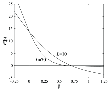
Figure 1: The topological pressure for a fully connected pentagon with $L=10$ and $L=70$ leads attached to each vertex. The velocity is $v=1$.

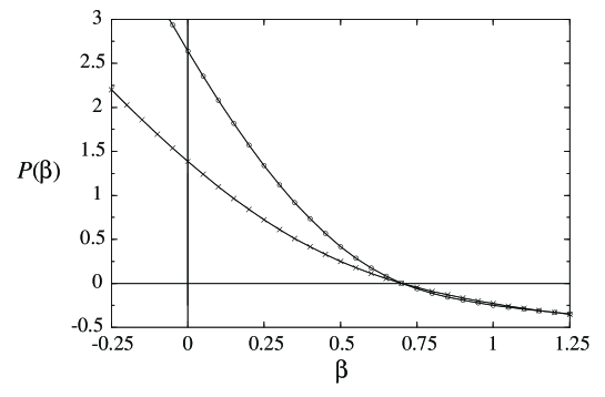
Figure 2: The topological pressure for a fully connected pentagon with $L=10$. The curve with the crosses is obtained when all bonds as unit length and the curve with the circles for a set of incommensurate lengths. The velocity is $v=1$.

6 Scattering on open graphs

We shall consider some examples that illustrate the previous concepts. Consider the fully connected pentagon with $L$ scattering leads attached to each vertex. Since the topological entropy $h_{\rm top}$ is independent of the Lyapunov exponents it is independent of the number of scattering leads attached to each vertex. This is observed in Fig. 1 where we depict the topological pressure for the fully connected pentagon.

Moreover, we observe that the escape rate $\gamma_{\rm cl}=-P(1)$ for the pentagon with $L=70$ is smaller than the escape rate for the pentagon with $L=10$. This behavior has a simple interpretation. Since we use $P_{bb^{\prime}}=\left|\frac{2}{\nu_{bb^{\prime}}}-\delta_{\hat{b^{\prime}}b^{\prime}}\right|^{2}$, the transmission probability from bond to bond decreases and the reflection probability increases as the valence of the vertex $\nu_{bb^{\prime}}$ increases. Therefore, as the number of leads increases, a particle on the pentagon has a smaller probability to escape and a larger probability to be reflected back to the same bond. Accordingly, the escape rate diminishes.

The examples of Fig. 2 shows that, indeed, the Hausdorff dimension is independent of the bond lengths.

As we see in these examples, the dynamics on typical graphs is characterized by a positive KS entropy $h_{\rm KS}>0$. In this sense, the classical dynamics on typical graphs is chaotic.

7 Diffusion on infinite periodic graphs

7.1 The hydrodynamic modes of diffusion

If the evolution of the density in an infinite periodic graph corresponds to a diffusion process, then the phenomenological diffusion equation should be satisfied in some limit. For instance, if the periodic graph forms a chain extending from $x=-\infty$ to $x=\infty$ then on a large scale (much larger than the period of the system) the density profile should evolve according to the diffusion equation

$$\frac{\partial\rho}{\partial t}=D\frac{\partial^{2}\rho}{\partial x^{2}}$$ (68)

Let us notice that $x$ is a one-dimensional coordinate of position along the graph which is a priori different from the position along each bond.

This equation admits solutions of the form

$$\rho_{k}=\exp\left[s(k)\;t\right]\exp(ikx)$$

with the dispersion relation

$$s(k)=-Dk^{2}$$ (69)

that relates the eigenvalue $s_{k}$ to the wave number $k$. These solutions are called the hydrodynamic modes of diffusion. The inverse of the wave number gives the wavelength $\ell=2\pi/k$ of the spatial inhomogeneities of concentration of particles.

For a system such as a graph, we expect deviations with respect to the diffusion equation which only gives the large-scale behavior of the probability density and not the behavior on the scale of the bonds. Moreover, we may also expect the existence of other kinetic modes of faster relaxation than the leading diffusive hydrodynamic mode. In order to obtain a full description of the relaxation, we have to compute the eigenvalues of the evolution operator for an infinite periodic graph. One of these eigenvalues will have the dependence of Eq. (69) for small $k$ which allows us to obtain from it the diffusion coefficient of the chain. We shall start by considering periodic graphs in a $d$-dimensional space to show the generality of the method but then we will specialize to periodic graphs that form one-dimensional chains.

7.2 Fourier decomposition of the Frobenius-Perron operator

In spatially extended systems which form a periodic lattice, spatial Fourier transforms are needed in order to reduce the dynamics to an elementary cell of the lattice [9]. In this reduction a wave number $\bf k$ is introduced for each hydrodynamic mode. The wave number characterizes a spatial quasiperiodicity of the probability density with respect to the lattice periodicity. Indeed, the wavelength of the mode does not need to be commensurate with the size of a unit cell of the lattice. Each Fourier component of the density evolves independently with an evolution operator that depends on $\bf k$. Accordingly, the Pollicott-Ruelle resonances will also depend on $\bf k$. We shall implement this reduction starting from the master equation (25) of the fully periodic graph and construct from it the evolution operator for the unit cell. A few new definitions are needed before proceeding with this construction.

The periodic graph is obtained by successive repetitions of a unit cell. Such graphs form a Bravais lattice $\mathcal{L}$. A lattice vector ${\bf a}_{\bf m}$ is centered in each cell of the Bravais lattice with ${\bf m}=(m_{1},m_{2},...,m_{d})\in{\mathbb{Z}}^{d}$. The lattice vectors are given by linear combinations of the basic vectors of the lattice

$${\bf a}_{\bf m}=m_{1}{\bf a}_{100\cdots 00}+m_{2}{\bf a}_{010\cdots 00}+\cdots+m_{d}{\bf a}_{000\cdots 01}\in\mathcal{L}$$

(for a one-dimensional chain we have $d=1$ and $a_{m}=m\in{\mathbb{Z}}$). We shall split the coordinate $[b,x]$ which refers to an arbitrary bond in the infinite graph into the new coordinates $([\mathrm{b},x],{\bf a})$ where the first pair refers to the equivalent position in the elementary unit cell to which the dynamics is reduced. That is, the bond $\mathrm{b}$ is associated with $b$ and $x$ is the position in that bond. The third term represents a vector in the Bravais lattice that gives the true position of the bond $b$ with respect to the position of the original unit cell, that is $b$ is obtained by translating the bond b to the cell in the Bravais lattice identified by the vector ${\bf a}$. We may introduce the notation $b=T_{\bf a}(\mathrm{b})$ where the translation operators $T_{\bf a}$ assign to a bond $\mathrm{b}$ the corresponding bond in the unit cell characterized by the vector ${\bf a}$.

Accordingly, the density in the graph is represented by a new function $\rho$ related to the old one by $\rho([{\mathrm{b}},x],{\bf a},t)=\rho([b,x],t)$.

We define a projection operator by

$$\hat{E}_{\bf k}=\sum_{{\bf a}\in\mathcal{L}}\exp(-i{\bf k}\cdot{\bf a})\hat{S}^{\bf a},$$ (70)

in terms of the spatial translation operators

$$\hat{S}^{\bf a}f([{\mathrm{b}},x],{\bf a}^{\prime},t)=f([{\mathrm{b}},x],{\bf a}^{\prime}+{\bf a},t)\quad\text{for}\ {\bf a},{\bf a}^{\prime}\in\mathcal{L}.$$

The projection operator (70) involves the so-called wave number ${\bf k}$. This later is defined on the Brillouin zone $\mathcal{B}$ of the reciprocal lattice $\widetilde{\mathcal{L}}$. The volume of the Brillouin zone is

$$|{\mathcal{B}}|=\int_{{\mathcal{B}}}d{\bf k}=\frac{(2\pi)^{d}}{\left|\det({\bf a}_{100\cdots 00},{\bf a}_{010\cdots 00},...,{\bf a}_{000\cdots 01})\right|}.$$

The operators (70) are projection operators since

$$\hat{E}_{\bf k}\hat{E}_{{\bf k}^{\prime}}=|\mathcal{B}|\;\delta({\bf k}-{\bf k}^{\prime})\hat{E}_{\bf k}$$

which is a consequence of the relation

$$\frac{1}{|\mathcal{B}|}\sum_{{\bf a}\in\mathcal{L}}\exp(i{\bf k}\cdot{\bf a})=\sum_{{\bf k}^{\prime}\in\widetilde{\mathcal{L}}}\;\delta({\bf k}-{\bf k}^{\prime}).$$

The identity operator is recovered by integrating the projection operator over the wave number

$$\hat{I}=\frac{1}{|\mathcal{B}|}\int d{\bf k}\;\hat{E}_{\bf k}.$$

If $\rho$ is the density defined on the infinite phase space, the function $\hat{E}_{\bf k}\rho$ is quasiperiodic on the lattice

$$\hat{E}_{\bf k}\rho([{\mathrm{b}},x],{\bf a},t)=\sum_{{\bf a}^{\prime}\in{\mathcal{L}}}\exp(-i{\bf k}\cdot{\bf a}^{\prime})\rho([{\mathrm{b}},x],{\bf a}+{\bf a}^{\prime},t)\\ =\exp(i{\bf k}\cdot{\bf a})\sum_{{\bf a}^{{}^{\prime\prime}}\in{\mathcal{L}}}\exp(-i{\bf k}\cdot{\bf a}^{{}^{\prime\prime}})\rho([{\mathrm{b}},x],{\bf a}^{{}^{\prime\prime}},t)\\ =\exp(i{\bf k}\cdot{\bf a})\hat{E}_{\bf k}\rho([{\mathrm{b}},x],{\bf 0},t)=\exp(i{\bf k}\cdot{\bf a})\rho_{\bf k}([{\mathrm{b}},x],t).$$

We have therefore a decomposition of the density over the infinite phase space into components defined in the reduced phase space and which depends continuously on the wave number ${\bf k}$.

Consider the master equation (25) of the full periodic graph. Applying at both sides the operator $\hat{E}_{\bf k}$ we get from the quasiperiodicity of $\hat{E}_{\bf k}\rho$ [see the previous equation]

$$\exp(i{\bf k}\cdot{\bf a}_{{\bf m}})\rho_{\bf k}([{\mathrm{b}},x],t)=\sum_{b^{\prime}}P_{bb^{\prime}}\exp(i{\bf k}\cdot{\bf a}_{{\bf m}^{\prime}})\rho_{\bf k}\left([{\mathrm{b}}^{\prime},x],t-\frac{x+l_{{\mathrm{b}}^{\prime}}-x^{\prime}}{v}\right).$$ (71)

where $b=T_{{\bf a}_{\bf m}}({\mathrm{b}})$ and $b^{\prime}=T_{{\bf a}_{{\bf m}^{\prime}}}({\mathrm{b}}^{\prime})$ and also $l_{b}=l_{{\mathrm{b}}}$. Now, the translational symmetry implies that

$$P_{bb^{\prime}}=P_{T_{{\bf a}_{\bf m}}({\mathrm{b}}),T_{{\bf a}_{{\bf m}^{\prime}}}({\mathrm{b}}^{\prime})}=P_{T_{{\bf a}_{\bf m-m^{\prime}}}({\mathrm{b}}),{\mathrm{b}}^{\prime}}$$

Thus Eq. (71) is

$$\rho_{{\bf k}}([{\mathrm{b}},x],t)=\sum_{{\mathrm{b}}^{\prime}}\sum_{{\bf m}^{\prime}}P_{T_{{\bf a}_{\bf m-m^{\prime}}}({\mathrm{b}}),{\mathrm{b}}^{\prime}}\;\exp(-i{\bf k}\cdot{\bf a}_{{{\bf m}}-{{\bf m^{\prime}}}})\ \rho_{{\bf k}}\left([{\mathrm{b}}^{\prime},x],t-\frac{x+l_{{\mathrm{b}}^{\prime}}-x^{\prime}}{v}\right)$$

The time evolution of the $\bf k$-component is therefore controlled by the matrix of elements

$${\mathrm{P}}_{\mathrm{bb}^{\prime}}({\bf k})\equiv\sum_{{\bf m}}P_{T_{{\bf a}_{\bf m}}({\mathrm{b}}),{\mathrm{b}}^{\prime}}\exp(-i{\bf k}\cdot{\bf a}_{{\bf m}})$$ (72)

We observe that, for a graph, there is at most one term in the sum of Eq. (72). Indeed, the coefficient $P_{T_{{\bf a}_{\bf m}}({\mathrm{b}}),{\mathrm{b}}^{\prime}}$ does not vanish if and only if the bonds $T_{{\bf a}_{\bf m}}({\mathrm{b}})$ and ${\mathrm{b}}^{\prime}$ are connected with the same vertex of the infinite graph. Furthermore, there is one and only one translation $T_{{\bf a}_{\bf m}}$ for which $T_{{\bf a}_{\bf m}}({\mathrm{b}})$ and ${\mathrm{b}}^{\prime}$ are connected with the same vertex. Accordingly, there exists a unique lattice vector ${\bf a}({\rm b},{\rm b}^{\prime})$ such that

$${\mathrm{P}}_{\mathrm{bb}^{\prime}}({\bf k})=P_{T_{{\bf a}({\rm b},{\rm b}^{\prime})}({\rm b}),{\rm b}^{\prime}}\exp\left[-i{\bf k}\cdot{\bf a}({\rm b},{\rm b}^{\prime})\right]$$ (73)

Thanks to this matrix, we have that each Fourier component of the density evolves with an equation

$$\rho_{{\bf k}}([{\mathrm{b}},x],t)=\sum_{{\mathrm{b}}^{\prime}}{\mathrm{P}}_{{\mathrm{bb}}^{\prime}}({\bf k})\;\rho_{{\bf k}}\left([{\mathrm{b}}^{\prime},x],t-\frac{x+l_{{\mathrm{b}}^{\prime}}-x^{\prime}}{v}\right)$$ (74)

Here the sum is carried out over all the directed bonds of the unit cell and the matrix ${\mathsf{P}}({\bf k})$ of elements $\mathrm{P}_{\mathrm{bb}^{\prime}}({\bf k})$ defined by Eq. (73) is a square matrix with dimension equal to the number of directed bonds in the unit cell.

7.3 The eigenvalue problem and the diffusion coefficient

To study the eigenvalues of the Frobenius-Perron operator $\hat{R}_{\bf k}^{t}$ defined by Eq. (74) we proceed as in Subsec. 3.2. We introduce the following definitions

$$\rho_{{\bf k},s}\left[{\mathrm{b}}\right]=\int_{0}^{\infty}\mbox{e}^{-st}\rho_{\bf k}\left(\left[{\mathrm{b}},0\right],t\right)dt$$

and

$$Q_{{\mathrm{b}}{\mathrm{b}}^{\prime}}(s,{\bf k})={\mathrm{P}}_{{\rm bb}^{\prime}}({\bf k})\;\exp\left(-s\frac{l_{{\mathrm{b}}^{\prime}}}{v}\right)$$ (75)

for the elements of the matrix ${\mathsf{Q}}(s,{\bf k})$. Then, taking the Laplace transform of Eq. (74) we get

$$\rho_{{\bf k},s}\left[{\mathrm{b}}\right]=\sum_{{\mathrm{b}}^{\prime}}Q_{{\mathrm{b}}{\mathrm{b}}^{\prime}}(s,{\bf k})\;\rho_{{\bf k},s}\left[{\mathrm{b}}^{\prime}\right]$$

which has a solution only if the following classical zeta function vanishes

$$Z(s;{\bf k})\equiv\det[{\mathsf{I}}-{\mathsf{Q}}(s,{\bf k})]=\prod_{p}\left[1-\mbox{e}^{-(\lambda_{p}+s)\frac{l_{p}}{v}-i{\bf k}\cdot{\bf a}_{p}}\right]=0$$ (76)

where the product extends over the prime periodic orbits $p$ of the unit cell of the graph and where ${\bf a}_{p}=\sum_{i=1}^{n_{p}}{\bf a}({\rm b}_{i+1},{\rm b}_{i})$ is the displacement on the lattice along the periodic orbit $p={\mathrm{b}}_{1}{\mathrm{b}}_{2}\cdots{\mathrm{b}}_{n_{p}}$ of prime period $n_{p}$. From Eq. (76), we obtain the functions $s_{j}({\bf k})$ and the corresponding eigenstates $\boldsymbol{\chi}_{j,{\bf k}}$ which satisfy

$$\boldsymbol{\chi}_{j,{\bf k}}={\mathsf{Q}}\left[s_{j}({\bf k}),{\bf k}\right]\cdot\boldsymbol{\chi}_{j,{\bf k}}.$$

Eq. (76) shows that the Pollicott-Ruelle resonances $s_{j}({\bf k})$ are the zeros of a new classical Selberg-Smale zeta function defined for the spatially periodic graphs. The eigenvalues and eigenstates of the Frobenius-Perron operator $\hat{R}_{{\bf k}}^{t}$ defined by Eq. (74) are constructed in the same way as in Subsec. 3.2. If we denote by $\Psi_{j,{\bf k}}[{\mathrm{b}},x]$ the eigenstates of the flow, the results are

$$\hat{R}_{{\bf k}}^{t}\Psi_{j,{\bf k}}[{\mathrm{b}},x]=\mbox{e}^{s_{j}({\bf k})t}\Psi_{j,{\bf k}}[{\mathrm{b}},x]$$

with

$$\Psi_{j,{\bf k}}[{\mathrm{b}},x]=\mbox{e}^{-s_{j}({\bf k})\frac{x}{v}}\chi_{j,{\bf k}}[{\mathrm{b}}]\qquad\mbox{for}\quad 0<x<l_{{\mathrm{b}}}$$

where $s_{j}({\bf k})$ is a solution of Eq. (76).

For ${\bf k}=0$, Eq. (74) represents the evolution of the density in the unit cell with periodic boundary conditions. The periodic boundary conditions transform two bonds in a loop. In this way, for ${\bf k}=0$, we are studying the evolution of a closed graph and we saw in Subsec. 3.2 that, for a closed graph, the value $s=0$ is a solution of Eq. (76) and the associated eigenstate corresponds to the invariant measure or equilibrium probability which is given by the $2B$-vector ($B$ being the number of bonds in the unit cell)

$$\boldsymbol{\chi}_{0}=\frac{1}{2B}(1,1,\ldots,1).$$ (77)

We may thus expect that, for $\bf k$ small enough, there exists a zero $s_{0}({\bf k})$ of Eq. (76) and a corresponding eigenstate

$$\boldsymbol{\chi}_{0,{\bf k}}={\mathsf{Q}}\left[s_{0}({\bf k}),{\bf k}\right]\cdot\boldsymbol{\chi}_{0,{\bf k}}$$ (78)

such that $s_{0}({\bf k})_{\overrightarrow{{\bf k}\rightarrow 0}}0.$ This particular resonance can be identified with the dispersion relation of the hydrodynamic mode of diffusion since this latter is known to vanish at ${\bf k}=0$ as

$$s_{0}({\bf k})=-\sum_{\alpha\beta}D_{\alpha\beta}k_{\alpha}k_{\beta}+{\mathcal{O}}({\bf k}^{4})$$

so that the diffusion matrix is obtained as

$$D_{\alpha\beta}=-\left.\frac{1}{2}\;\frac{\partial^{2}s_{0}({\bf k})}{\partial k_{\alpha}\partial k_{\beta}}\right|_{{\bf k}=0}$$ (79)

7.4 Example of infinite graph with diffusion

We illustrate the results of this section with a very simple example of a one-dimensional chain. Consider the graph used in Subsubsec. 4.3.2. This graph of scattering type can be used as a unit cell for a periodic graph. The right lead is connected with the left lead of an equivalent graph and so on. This graph looks like an infinite comb. The unit cell can be considered as composed by two bonds, say $b$ and $a$. The bond $b$ connects the dead vertex $2$ with the vertex $1$ and the bond $a$ connects the vertex $1$ with the vertex $1$ of the next cell. Thus the valence of the vertices are $v_{2}=1$ and $v_{1}=3$ respectively. The transition probabilities $P_{bb^{\prime}}$ are given by

$$P_{bb^{\prime}}=\left|T_{bb^{\prime}}\right|^{2}$$

with, $P_{b\hat{b}}=1,P_{ab}=\frac{4}{9},P_{\hat{b}b}=\frac{1}{9},P_{a\hat{a}}=\frac{1}{9},P_{\hat{b}\hat{a}}=\frac{4}{9},P_{\hat{a}a}=\frac{1}{9}$ and zero otherwise. We first construct the matrix ${\mathrm{P}}(k)$. We note from its definition in Eq. (73) that ${\mathrm{P}}_{\mathrm{bb}^{\prime}}(k)=P_{{bb}^{\prime}}$ for bonds that belong to the unit cell. The $k$-dependent factors come from bonds that connect consecutive cells. These bonds are:

• The bond $a$ of the cell at the left-hand side characterized by $a_{m}=-1$ is connected with the bonds $a$ and $\hat{b}$. This gives the contributions ${\mathrm{P}}_{{\rm aa}}(k)=\frac{4}{9}\mbox{e}^{+ik}$ and ${\mathrm{P}}_{\hat{\rm b}{\rm a}}(k)=\frac{4}{9}\mbox{e}^{+ik}$.

• The bonds $\hat{a}$ and $b$ of the cell at the right-hand side characterized by $a_{m}=+1$ are connected with the bond $\hat{a}$. This gives the contributions ${\mathrm{P}}_{\hat{\rm a}\hat{\rm a}}(k)=\frac{4}{9}\mbox{e}^{-ik}$ and ${\mathrm{P}}_{\hat{\rm a}{\rm b}}(k)=\frac{4}{9}\mbox{e}^{-ik}$.

Therefore, ${\mathsf{P}}(k)$ is the $4\times 4$ matrix with entries

$${\mathsf{P}}(k)=\left[\begin{array}[]{cccc}0&1&0&0\\ \frac{1}{9}&0&\frac{4}{9}\mbox{e}^{ik}&\frac{4}{9}\\ \frac{4}{9}&0&\frac{4}{9}\mbox{e}^{ik}&\frac{1}{9}\\ \frac{4}{9}\mbox{e}^{-ik}&0&\frac{1}{9}&\frac{4}{9}\mbox{e}^{-ik}\end{array}\right]$$

where the columns and rows are arranged in the following order $\rm(b,\hat{b},a,\hat{a})$. The matrix ${\mathsf{Q}}(s,k)$ is obtained by multiplication with the diagonal matrix $\delta_{\rm bb^{\prime}}\mbox{e}^{-\frac{s}{v}l_{\rm b^{\prime}}}$. The determinant in Eq. (76) can be computed and gives

$$\det\left[{\mathsf{I}}-{\mathsf{Q}}(s,k)\right]=1+\frac{5}{27}\mbox{e}^{-2\frac{s}{v}a}-\frac{1}{9}\mbox{e}^{-2\frac{s}{v}g}+\frac{1}{9}\mbox{e}^{-2\frac{s}{v}(a+g)}-\frac{8}{9}\mbox{e}^{-\frac{s}{v}a}\left(1+\frac{\mbox{e}^{-2\frac{s}{v}g}}{3}\right)\cos k$$ (80)

where $a$ is the length of the bond $\rm a$ and $g$ is the length of the bond $\rm b$. As we said the solutions of $\det\left[{\mathsf{I}}-{\mathsf{Q}}(s,k)\right]=0$ gives the desired functions $s_{j}(k)$. For this example, we plot the first branches in Fig. 3 where we observe that, indeed, only one branch includes the point $s=0$ at $k=0$. This unique branch can be identified with the dispersion relation of the hydrodynamic mode of diffusion.

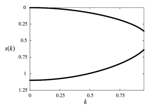
Figure 3: The first two branches $s(k)$ of Pollicott-Ruelle resonances of the infinite comb graph, as obtained from Eq. (80). The branch containing the origin $s=0$ and $k=0$ is the dispersion relation of the diffusive mode. The other branch is associated with a kinetic mode of faster relaxation.

The diffusion coefficient is obtained from the second derivative of the first branch at $k=0$. This can be analytically computed for this particular example as follows. We consider $s<<{\rm Min}\{v/a,v/g\}$ and $k<<1$ and expand Eq. (80). After some simple algebra, we get

$$\det\left[{\mathsf{I}}-{\mathsf{Q}}(s,k)\right]=\frac{16}{27}\left[\frac{s}{v}(a+g)+k^{2}\right]+{\cal O}(s^{2})+{\cal O}(sk^{2})+{\cal O}(k^{4})$$

from which we obtain that the diffusion coefficient defined by Eq. (79) is

$$D=\frac{v}{a+g}$$ (81)

In general, the diffusion coefficient has the units of $[L^{2}]/[T].$ This is because the wave number has the units of $1/[L]$. Since we have considered $k$ as a dimensionless number, the diffusion coefficient has here the units of $1/[T]$. In this example the standard units can be recovered by considering $k=\kappa a$ with a standard wave number $\kappa$ where $a$ is the period at which the unit cell is repeated. In these units, we would have obtained $\tilde{D}=v\frac{a^{2}}{a+g}$. But, in general, for a more complicated graph, there is no bond length that we can associate with the periodicity of the chain as in this example, which is the reason why we consider the dimensionless parameter $k$. In this sense we are considering the space in units of the unit cell of the periodic chain.

7.5 A Green-Kubo formula for the diffusion coefficient

In the previous example, we have seen that the diffusion coefficient is inversely proportional to the total length of the unit cell. This is a general property that follows from a general expression for the diffusion coefficient that we shall now obtain. From now on we shall consider one-dimensional chains. Accordingly, $k$ is a scalar wavenumber and no longer a vector.

Consider the vector $\boldsymbol{\chi}_{0,k}$ defined by Eq. (78) and the eigenvector $\tilde{\boldsymbol{\chi}}_{0,k}$ of the adjoint matrix ${\mathsf{Q}}\left[s_{0}(k),k\right]^{\dagger}$ defined by

$${\mathsf{Q}}\left[s_{0}(k),k\right]^{\dagger}\cdot\tilde{\boldsymbol{\chi}}_{0,k}=\tilde{\boldsymbol{\chi}}_{0,k}$$ (82)

or equivalently

$$\tilde{\boldsymbol{\chi}}_{0,k}^{\dagger}=\tilde{\boldsymbol{\chi}}_{0,k}^{\dagger}\cdot{\mathsf{Q}}\left[s_{0}(k),k\right]$$ (83)

This eigenvector satisfies

$$\tilde{\chi}_{0,k}[{\mathrm{b}}]_{\ \overrightarrow{k\rightarrow 0}}\ 1$$ (84)

Such vectors are normalized as

$$(\tilde{\boldsymbol{\chi}}_{0,k},\boldsymbol{\chi}_{0,k})=\sum_{{\mathrm{b}}}\tilde{\chi}_{0,k}[{\mathrm{b}}]^{\ast}\chi_{0,k}[{\mathrm{b}}]=1$$ (85)

On the other hand, due to Eqs. (78) and (82), we have

$$\left(\tilde{\boldsymbol{\chi}}_{0,k},{\mathsf{Q}}\left(s_{0},k\right)\cdot\boldsymbol{\chi}_{0,k}\right)=1.$$ (86)

with $s_{0}=s_{0}(k)$. Differentiating Eq. (85) and Eq. (86) with respect to $k$ we get respectively

$$\left(\frac{d\tilde{\boldsymbol{\chi}}_{0,k}}{dk},\boldsymbol{\chi}_{0,k}\right)+\left(\tilde{\boldsymbol{\chi}}_{0,k},\frac{d\boldsymbol{\chi}_{0,k}}{dk}\right)=0$$

and

$$\left(\frac{d\tilde{\boldsymbol{\chi}}_{0,k}}{dk},\boldsymbol{\chi}_{0,k}\right)+\left(\tilde{\boldsymbol{\chi}}_{0,k},\left[\frac{d}{dk}{\mathsf{Q}}(s_{0},k)\right]\cdot\boldsymbol{\chi}_{0,k}\right)+\left(\tilde{\boldsymbol{\chi}}_{0,k},\frac{d\boldsymbol{\chi}_{0,k}}{dk}\right)=0$$

where we have used Eqs. (78) and (82). These last two equations imply

$$\left(\tilde{\boldsymbol{\chi}}_{0,k},\left[\frac{d}{dk}{\mathsf{Q}}(s_{0},k)\right]\cdot\boldsymbol{\chi}_{0,k}\right)=\sum_{{\mathrm{b,b}}^{\prime}}\tilde{\chi}_{0,k}[{\mathrm{b}}]^{\ast}\left[\frac{d}{dk}Q_{{\mathrm{bb}}^{\prime}}(s_{0},k)\right]\chi_{0,k}[{\mathrm{b}}^{\prime}]=0$$ (87)

Now we compute the derivative of $\mathsf{Q}$. From Eq. (75) and Eq. (73), we have

$$\frac{d}{dk}Q_{{\mathrm{bb}}^{\prime}}(s_{0},k)=\left[\frac{d}{dk}{\mathrm{P}}_{{\mathrm{bb}}^{\prime}}(k)\right]\exp\left(-s_{0}\frac{l_{{\mathrm{b}}^{\prime}}}{v}\right)-Q_{{\mathrm{bb}}^{\prime}}(s_{0},k)\frac{l_{{\mathrm{b}}^{\prime}}}{v}\frac{ds_{0}}{dk}.$$

Inserting this result into Eq. (87) and taking the limit $k\rightarrow 0$, we obtain

$$\left.\frac{ds_{0}}{dk}\right|_{k=0}=\frac{\frac{1}{2B}\sum_{{\mathrm{b,b}}^{\prime}}\left.\frac{d{\mathrm{P}}_{{\mathrm{bb}}^{\prime}}}{dk}\right|_{k=0}}{\frac{1}{2B}\sum_{{\mathrm{b,b}}^{\prime}}\left.{\mathrm{P}}_{{\mathrm{bb}}^{\prime}}\right|_{k=0}\frac{l_{{\mathrm{b}}^{\prime}}}{v}},$$

where we have used the fact that the limit $k\rightarrow 0$ implies $s_{0}(k)\rightarrow 0$, and that $\chi_{0,k}[{\mathrm{b}}^{\prime}]\rightarrow\frac{1}{2B},\tilde{\chi}_{0,k}[{\mathrm{b]}\rightarrow 1}$ because of Eqs. (77) and (84). Since $\sum_{{\mathrm{b}}}\left.{\mathrm{P}}_{{\mathrm{bb}}^{\prime}}\right|_{k=0}=1$, $\forall\,{\mathrm{b}}^{\prime}$, this reduces to:

$$\left.\frac{ds_{0}}{dk}\right|_{k=0}=\frac{v}{L_{{\mathrm{uc}}}}\sum_{{\mathrm{b,b}}^{\prime}}\left.\frac{d{\mathrm{P}}_{{\mathrm{bb}}^{\prime}}}{dk}\right|_{k=0}=0$$ (88)

where $L_{{\mathrm{uc}}}=\sum_{{\mathrm{b}}}l_{{\mathrm{b}}}$ is the total length of the unit cell. The last equality $(=0)$ follows from the fact that the unit cell is connected with the neighboring cells in a symmetric way. For instance, in a one-dimensional chain, the “fluxes” from the left-hand side equal those from the right-hand side and the derivative with respect to $k$ drops a sign that makes the sum vanishing. The reader can verify this property in the previous example of the comb graph.

To obtain the diffusion coefficient we need the second derivative of $s_{0}(k)$. Therefore, we differentiate Eq. (87) with respect to $k$ and we evaluate at $k=0$. After some algebra and using Eq. (88), we get

$$\left.\frac{d^{2}s_{0}}{dk^{2}}\right|_{k=0}=\frac{v}{L_{\mathrm{uc}}}\left[\sum_{\mathrm{b,b}^{\prime}}\left.\frac{d^{2}\mathrm{P}_{\mathrm{bb}^{\prime}}}{dk^{2}}\right|_{k=0}+\sum_{\mathrm{b,b}^{\prime}}\left.\frac{d\mathrm{P}_{\mathrm{bb}^{\prime}}}{dk}\left(2B\frac{d\chi_{0,k}[\mathrm{b}^{\prime}\mathrm{]}}{dk}+\frac{d\tilde{\chi}_{0,k}[\mathrm{b}]^{\ast}}{dk}\right)\right|_{k=0}\right]$$ (89)

The explicit form for the diffusion coefficient is obtained from Eq. (89) if we compute the first derivatives of the eigenstates. We can write the equations that these quantities satisfy. In fact taking the derivative with respect to $k$ of Eqs. (78) and (83) we have

$$\frac{d\chi_{0,k}[{\mathrm{b}}]}{dk}=\sum_{{\mathrm{b}}^{\prime}}\frac{dQ_{{\mathrm{bb}}^{\prime}}}{dk}\chi_{0,k}[{\mathrm{b}}]+\sum_{{\mathrm{b}}^{\prime}}Q_{{\mathrm{bb}}^{\prime}}\frac{d\chi_{0,k}[{\mathrm{b}}^{\prime}]}{dk}$$

and

$$\frac{d\tilde{\chi}_{0,k}[{\mathrm{b}}^{\prime}]^{\ast}}{dk}=\sum_{{\mathrm{b}}}\tilde{\chi}_{0,k}[{\mathrm{b}}]^{\ast}\frac{dQ_{\mathrm{bb}^{\prime}}}{dk}+\sum_{\mathrm{b}}\frac{d\tilde{\chi}_{0,k}[{\mathrm{b}}]^{\ast}}{dk}Q_{\mathrm{bb}^{\prime}}$$

whose solutions are

$$\frac{d\chi_{0,k}[{\mathrm{b}}]}{dk}=\sum_{\mathrm{b^{\prime}}\mathrm{b^{\prime\prime}}}\left({\mathsf{I}}-{\mathsf{Q}}\right)_{\mathrm{bb}^{\prime}}^{-1}\frac{dQ_{\mathrm{b^{\prime}b}^{\prime\prime}}}{dk}\chi_{0,k}[\mathrm{b}^{\prime\prime}]$$

$$\frac{d\tilde{\chi}_{0,k}[{\mathrm{b}}]^{\ast}}{dk}=\sum_{\mathrm{b^{\prime}}\mathrm{b^{\prime\prime}}}\tilde{\chi}_{0,k}[{\mathrm{b}}^{\prime}]^{\ast}\frac{dQ_{\mathrm{b^{\prime}b}^{\prime\prime}}}{dk}\left({\mathsf{I}}-{\mathsf{Q}}\right)_{\mathrm{b^{\prime\prime}b}}^{-1}$$

In the limit $k\rightarrow 0$, these solutions can be written as

$$\left.\frac{d\chi_{0,k}[{\rm b}]}{dk}\right|_{k=0}=\frac{1}{2B}\sum_{{\rm b}^{\prime},{\rm b}^{\prime\prime}}\sum_{n=0}^{\infty}\left[\left({\mathsf{P}}^{n}\right)_{\mathrm{b,b^{\prime}}}\frac{d{\mathrm{P}}_{{\rm b}^{\prime},{\rm b}^{\prime\prime}}}{dk}\right]_{k=0}$$

and similarly

$$\left.\frac{d\tilde{\chi}_{0,k}[{\rm b}]^{\ast}}{dk}\right|_{k=0}=\sum_{{\rm b}^{\prime},{\rm b}^{\prime\prime}}\sum_{n=0}^{\infty}\left[\frac{d{\mathrm{P}}_{{\rm b}^{\prime},{\rm b}^{\prime\prime}}}{dk}\left({\mathsf{P}}^{n}\right)_{{\rm b}^{\prime\prime},{\rm b}}\right]_{k=0}$$

Thus, the second term of Eq. (89) becomes

$$\sum_{\mathrm{b,b}^{\prime}}\left.\frac{d\mathrm{P}_{\mathrm{bb}^{\prime}}}{dk}\left(2B\frac{d\chi_{0,k}[\mathrm{b}^{\prime}]}{dk}+\frac{d\tilde{\chi}_{0,\mathrm{k}}[\mathrm{b}]^{\ast}}{dk}\right)\right|_{k=0}\\ =2\sum_{\mathrm{b,b^{\prime},b^{\prime\prime},b^{\prime\prime\prime}}}\sum_{n=0}^{\infty}\left[\frac{d{\mathrm{P}}_{\mathrm{bb^{\prime}}}}{dk}\left({\mathsf{P}}^{n}\right)_{\mathrm{b^{\prime},b^{\prime\prime}}}\frac{d\mathrm{P}_{\mathrm{b^{\prime\prime}b^{\prime\prime\prime}}}}{dk}\right]_{k=0}$$

To evaluate and interpret this result we have to transform these expressions. First, we have to consider the derivatives of ${\mathsf{P}}(k)$. This matrix is defined in Eq. (73). Since only the nearest neighbors are connected, the lattice vector of the jumps can take only the values $a({\rm b},{\rm b}^{\prime})=0,\pm 1$ whether the particle crosses the boundary of the unit cell to the right-hand cell (+1), or the left-hand one (-1), or it stays in the same cell (0) during the transition ${\rm b}^{\prime}\to{\rm b}$. Therefore

$${\mathrm{P}}_{{\rm bb}^{\prime}}(k)=P_{T_{a({\rm b},{\rm b}^{\prime})}({\rm b}),{\mathrm{b}^{\prime}}}\ \mbox{e}^{-ika({\rm b},{\rm b}^{\prime})}$$

The derivatives of this matrix are thus

$$\frac{d{\mathrm{P}}_{\mathrm{bb^{\prime}}}}{dk}=-i\;a({\rm b},{\rm b}^{\prime})\ {\mathrm{P}}_{{\rm bb}^{\prime}}$$

and

$$\frac{d^{2}{\mathrm{P}}_{\mathrm{bb^{\prime}}}}{dk^{2}}=-a({\rm b},{\rm b}^{\prime})^{2}\ {\mathrm{P}}_{{\rm bb}^{\prime}}.$$

Accordingly, the diffusion coefficient is given by

$$D=-\frac{1}{2}\left.\frac{d^{2}s_{0}}{dk^{2}}\right|_{k=0}=\frac{v}{2{L}_{\mathrm{uc}}}\sum_{\mathrm{b,b^{\prime}}}\biggl{[}a({\rm b},{\rm b}^{\prime})^{2}{\mathrm{P}}_{\mathrm{bb^{\prime}}}\\ +2\sum_{\mathrm{b^{\prime\prime}b^{\prime\prime\prime}}}\sum_{n=0}^{\infty}a({\rm b},{\rm b}^{\prime}){\mathrm{P}}_{\mathrm{bb^{\prime}}}\left({\mathsf{P}}^{n}\right)_{\mathrm{b^{\prime},b^{\prime\prime}}}a({\mathrm{b^{\prime\prime}}},{\mathrm{b^{\prime\prime\prime}}}){\mathrm{P}}_{\mathrm{b^{\prime\prime}b^{\prime\prime\prime}}}\biggr{]}_{k=0}$$ (90)

In order to interpret this formula, we have to remember some definitions. If an observable is defined over $M$ successive bonds, its mean value over the equilibrium invariant measure of the random process is given by

$$\left\langle A\right\rangle=\lim_{N\rightarrow\infty}\sum_{b_{-N}\cdots b_{N}}A(b_{M-1}\cdots b_{1}b_{0})\;\mu(b_{N}\cdots b_{-N}).$$ (91)

If the observable $A$ depends only on two consecutive bonds as it is the case for the jump vector $a({\rm b},{\rm b}^{\prime})$, its mean value takes the form

$$\left\langle A\right\rangle=\sum_{b_{0}b_{1}}A(b_{1}b_{0})\;\mu(b_{1}b_{0})=\sum_{b_{0}b_{1}}A(b_{1}b_{0})\;P_{b_{1}b_{0}}\;\chi_{0}[b_{0}]=\frac{1}{2B}\sum_{b_{0}b_{1}}A(b_{1}b_{0})\;P_{b_{1}b_{0}}$$

because of Eqs. (52) and (77). According to the general definition (91), the time-discrete autocorrelation function of a two-bond observable is given by

$$\left\langle A_{m}A_{0}\right\rangle=\sum_{b_{0}\cdots b_{m+1}}A(b_{m+1}b_{m})A(b_{1}b_{0})\;\mu(b_{m+1}b_{m}\cdots b_{1}b_{0})$$

Because of Eqs. (52) and (77) again, we get

$$\left\langle A_{m}A_{0}\right\rangle=\frac{1}{2B}\sum_{b_{0}b_{1}b_{m}b_{m+1}}A(b_{m+1}b_{m})P_{b_{m+1}b_{m}}\left({\mathsf{P}}^{m-1}\right)_{b_{m}b_{1}}A(b_{1}b_{0})\;P_{b_{1}b_{0}}$$ (92)

The terms of Eq. (90) are precisely of the form of Eq. (92) with $m=0$ for the first term and $m=n+1$ for the following ones, and with the observable $A=a$. Since the process is stationary we have that $\left\langle a_{n}a_{0}\right\rangle=\left\langle a_{0}a_{-n}\right\rangle=\left\langle a_{-n}a_{0}\right\rangle$ where the last equality follows from the commutativity of the quantities $a_{0}$ and $a_{-n}$. Therefore, the term with the sum over $n$ in Eq. (90) is equal to $2B\sum_{n=-\infty,n\neq 0}^{+\infty}\left\langle a_{0}a_{n}\right\rangle$. It is now clear that Eq. (90) for the diffusion coefficient is

$$D=\frac{Bv}{L_{\mathrm{uc}}}\sum_{n=-\infty}^{+\infty}\left\langle a_{0}a_{n}\right\rangle=\frac{v}{2\left\langle l\right\rangle}\sum_{n=-\infty}^{+\infty}\left\langle a_{0}a_{n}\right\rangle$$ (93)

where $\left\langle l\right\rangle=L_{\rm uc}/(2B)$ is the mean bond-length of the unit cell and $a_{n}=0,\pm 1$ is the jump from one cell to another undergone by the particle in motion on the infinite graph.

Eq. (93) is nothing else than the Green-Kubo formula for the diffusion coefficient. If we define

$$v_{x}=\frac{\Delta x}{\Delta t}=\frac{v}{\left\langle l\right\rangle}\;a({\rm b},{\rm b}^{\prime})$$

as the velocity along the $x$-axis that contributes to the transport, where $\Delta t=\left\langle l\right\rangle/v$, we can write Eq. (93) in the more familiar Green-Kubo form

$$D=\frac{1}{2}\int_{-\infty}^{+\infty}\left\langle v_{x}(0)v_{x}(t)\right\rangle dt.$$

In the time-discrete form (93), we obtain the result that the diffusion coefficient is proportional to the constant velocity $v$ and inversely proportional to the mean bond-length of a unit cell. The diffusion coefficient is also proportional to the sum of the time-discrete autocorrelation of the jump $a$ from cell to cell.

8 Escape and diffusion on large open graphs

In this section, we shall study the Pollicott-Ruelle resonances of open graphs characterized by a unit cell which is repeated a finite number of times. The particular example that we consider is depicted in Fig. 4. We shall focus on the leading resonance that determines the escape rate from the system. We shall show that, for large enough chains (i.e., made of several unit cells), the classical lifetime corresponds to the time spent by a particle that undergoes a diffusive process in the chain before it escapes.

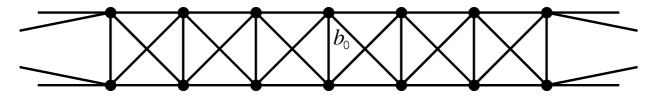
Figure 4: Open graph forming a chain composed of $N=6$ identical unit cells. The five lengths that compose the unit cell take different values. (In this regard, no specific length can be associated with the periodicity of the chain.)

For the graph of Fig. 4, the transition probabilities from bond to bond $P_{bb^{\prime}}$ are given by

$$P_{bb^{\prime}}=\left\{\begin{array}[]{l}\frac{9}{25}\text{ if the particle is reflected, i.e., }b=b^{\prime}\;;\\ \frac{4}{25}\text{ for bonds }b\neq b^{\prime}\text{ which are connected}\;;\\ 0\ \text{ otherwise}\;.\end{array}\right.$$

We have computed the spectrum of Pollicott-Ruelle resonances for different values of the number $N$ of unit cells. The leading resonance controls the asymptotic decay. Since the leading resonance is isolated and at a finite distance from the real axis the decay is exponential as we explained, that is

$$\rho(t)\sim\exp\left(-\gamma_{\rm cl}t\right)$$

where $\gamma_{\rm cl}$ is the leading resonance, i.e., the escape rate. This is the generic behavior of the density in a classically chaotic open system and we refer to this as the classical decay.

In Fig. 5, we depict the topological pressure for the chain of Fig. 4 with $N=7$ unit cells.

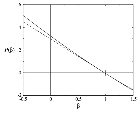
Figure 5: Topological pressure for the chain of Fig. 4 but with $N=7$. From this function, we get that $h_{\rm KS}\approx 2.9>0$ and $h_{\rm top}=3.2330$.

When the chaotic dynamics is at the origin of a diffusion process the escape rate is inversely proportional to the square of the size of the system, more precisely the following relation is expected to hold

$$\gamma_{\rm cl}(N)\simeq D\;\frac{\pi^{2}}{N^{2}}$$ (94)

with $D$ the diffusion coefficient. As explained in Sec. 5, the escape rate is related to the mean Lyapunov exponent and the KS entropy of the open chain of size $N$ according to

$$\gamma_{\rm cl}(N)=\lambda(N)-h_{\rm KS}(N)$$ (95)

As a consequence of Eq. (94), we find also for open graphs a known relationship between the diffusion coefficient and the chaotic properties [18]

$$D=\lim_{N\to\infty}\frac{N^{2}}{\pi^{2}}\;\left[\lambda(N)-h_{\rm KS}(N)\right]$$ (96)

Here again $D$ is in units of $[1]/[T]$ because we did not associate a length with the period of the chain and thus the space is in units of unit cell.

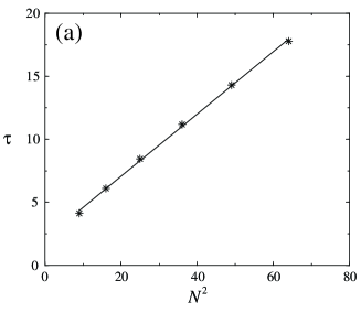
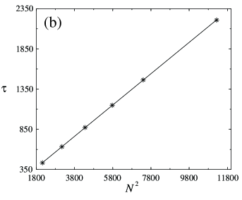
Figure 6: Lifetime of the chain of Fig. 4 as a function of the square of its size $N$: (a) For $N=3,4,5,6,7,8$, the slope of the linear regression is $0.247403$ and Eq. (94) gives an approximate diffusion coefficient $D\simeq 0.4095$. (b) For $N=46,56,66,76,86,106$, the slope of the linear regression is $0.1946247$ and Eq. (94) gives a better approximation $D\simeq 0.5205$ for the diffusion coefficient (97).

We have computed the escape rate for chains of different sizes. If the dynamics indeed corresponds to a diffusion process, then Eq. (94) should be verified. In figure 6, we plot the classical lifetimes $\tau_{\rm cl}$ as a function of $N^{2}$. Since $\tau_{\rm cl}=1/\gamma_{\rm cl}$, we observe the dependence of $\gamma_{\rm cl}$ on $N$ expected from Eq. (94). We may conclude from this result that the classical dynamics in the open chain is the one of a diffusion process.

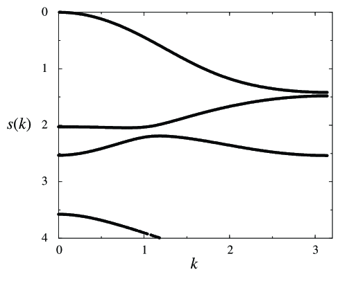
Figure 7: The first branches $s(k)$ of Pollicott-Ruelle resonances of the infinite graph corresponding to the open graph of Fig. 4. Here again we observe that there is only one branch that is identified with the hydrodynamic mode of diffusion, $s_{0}(k)$, because it vanishes for $k=0$.

The diffusion coefficient of the infinite graph can be obtained as we explained in Sec. 7. We depict in Fig. 7 the leading and other Pollicott-Ruelle resonances of the infinite graph obtained by numerical calculation as a function of the dimensionless wave number $k$. The diffusion coefficient is given by the second derivative of the leading resonance $s_{0}(k)$ evaluated at $k=0$. In this way, we obtain the numerical result

$$D=0.5318.$$ (97)

Accordingly, the diffusion coefficient of the infinite chain gives a reasonable estimate for the proportionality coefficient between $\gamma_{\rm cl}$ and $1/N^{2}$ for the small chains of Fig. 6a and is a very good estimate for the large chains of Fig. 6b.

In Fig. 8, we show how the effective diffusion coefficient $D(N)=\gamma_{\rm cl}(N)(N/\pi)^{2}$ converges to the diffusion coefficient of the infinite chain $D$, as the chain becomes longer and longer ($N\to\infty$).

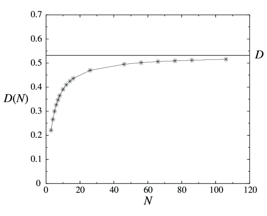
Figure 8: The effective diffusion coefficient $D(N)=\gamma_{\rm cl}(N)(N/\pi)^{2}$ as a function of $N$ for the open graphs of Fig. 4.

9 Diffusion in disordered graphs

In a recent work, Schanz and Smilansky [19] have considered the problem of Anderson localization in a one-dimensional graph composed of successive bonds of random lengths with random transmission and reflection coefficients at the vertices. The classical dynamics corresponding to this quantum model defines a kind of Lorentz lattice gases as studied in Refs. [20, 21]. Indeed, these references describe Lorentz lattice gases consisting of a moving particle traveling with allowed velocities $\pm v$ on a one-dimensional lattice of scatterers. If the particle arrives at a scatterer it will be transmitted or reflected with probabilities $p$ and $q=1-p$ respectively. If the scatterers are randomly distributed the model describes the classical dynamics of the model by Schanz and Smilansky with identical transmission and reflection coefficients at all the scatterers.

The classical dynamics of this model can be analyzed with the methods developed in the present paper, which provides the relationship with the cited works on the Lorentz lattice gases. Using the methods of Sec. 4, we can write down the infinite matrix ${\mathsf{Q}}(s)$. The eigenstates of this matrix corresponding to the unit eigenvalue can be obtained by iteration along the chain according to $\chi[b]=\exp(sl_{b}/2v)u_{b}$ and $\chi[\hat{b}]=\exp(sl_{b}/2v)u_{\hat{b}}$ with

$$\left(\begin{array}[]{c}u_{\hat{b}}\\ u_{b}\end{array}\right)={\mathsf{M}}_{b}\cdot\left(\begin{array}[]{c}u_{\widehat{b-1}}\\ u_{b-1}\end{array}\right)$$ (98)

where $b\in{\mathbb{Z}}$ and the matrix is defined by

$${\mathsf{M}}_{b}={\mathsf{B}}_{b}^{1/2}\cdot{\mathsf{V}}_{b-1}\cdot{\mathsf{B}}_{b-1}^{1/2}$$ (99)

with

$${\mathsf{V}}_{b-1}=\left(\begin{array}[]{cc}\frac{1}{p_{b}}&-\frac{q_{b}}{p_{b}}\\ \frac{q_{b}}{p_{b}}&1-\frac{q_{b}}{p_{b}}\end{array}\right)$$ (100)

and

$${\mathsf{B}}_{b}=\left(\begin{array}[]{cc}\mbox{e}^{+\frac{sl_{b}}{v}}&0\\ 0&\mbox{e}^{-\frac{sl_{b}}{v}}\end{array}\right)$$ (101)

We notice that $\det{\mathsf{M}}_{b}=1$. If the chain was periodic $l_{b}=l$, we would obtain the diffusion coefficient $\tilde{D}=vlp/(2q)$ by assuming that $u_{b+1}=\exp(i\kappa l)u_{b}$ in Eq. (98). In the dilute gas limit, the mean-field diffusion coefficient for the random graph is then given by replacing the bond length $l$ by the mean bond length $\langle l\rangle$, leading to:

$$\tilde{D}_{\rm mf}=v\;\langle l\rangle\;\frac{p}{2q}$$ (102)

For a disordered chain with $N$ scatterers, the Pollicott-Ruelle resonances can be obtained by finding the resonances $s$ for which the following equation is satisfied:

$$\left(\begin{array}[]{c}u_{\widehat{N+1}}\\ u_{N+1}\end{array}\right)=\prod_{b=1}^{N}{\mathsf{M}}_{b}(s)\cdot\left(\begin{array}[]{c}u_{\hat{1}}\\ u_{1}\end{array}\right)$$ (103)

If the chain closes on itself, we must impose the periodic boundary conditions $u_{\widehat{N+1}}=u_{\hat{1}}$ and $u_{N+1}=u_{1}$. If the chain is open and extended by two semi-infinite leads, we must consider the absorbing boundary conditions $u_{\widehat{N+1}}=0$ and $u_{1}=0$.

In Ref. [20], Ernst et al. have characterized the chaotic properties in such open graphs thanks to the escape-rate formalism by computing the topological pressure function of Sec. 5. In Ref. [21], Appert et al. showed that the spatial disorder is at the origin of a dynamical phase transition associated with a singularity in the pressure function of the infinite disordered chain.

10 Conclusions

In this paper, we have introduced and studied the random classical dynamics of a particle moving in a graph. We shall show elsewhere [11] that the dynamics here studied is the classical limit of the quantum dynamics introduced in Refs. [1, 2].

We have shown that the relaxation rates of the time-continuous classical dynamics can be obtained by a simple secular equation which includes the lengths of the bonds and the velocity of the particle. This secular equation has been directly related to the eigenvalue problem of the time-continuous Frobenius-Perron operator. The secular equation can be written as a classical zeta function defined as a product over the periodic orbits of the graphs. In this way, we have been able to define the relaxation rates, as well as chaotic properties such as the Lyapunov exponents and the entropies as quantities per unit of the continuous time. The chaotic properties are derived from a pressure function defined for each graph.

For infinite periodic graphs, we have shown how to construct the hydrodynamic modes of diffusion and to compute a diffusion coefficient. Here also, the relaxation rates of the hydrodynamic modes are given by the zeros of a classical zeta function. Moreover, a Green-Kubo formula for the diffusion coefficient has been deduced from the eigenvalue problem for the Frobenius-Perron operator of the classical dynamics on the graph.

When the chain is open by considering a finite segment connected with scattering leads, the particle escapes after a diffusion process. In this case, we have computed the lifetime of the metastable states. This classical lifetime is given by the inverse of the escape rate which is related to the diffusion coefficient. Accordingly, a known relationship between the diffusion coefficient and the chaotic properties [18] is extended to the random classical dynamics on graphs. The case of infinite disordered graphs has also be considered.

The interest of these results lies notably in the fact that the classical quantities here computed can be compared to equivalent quantities defined for the corresponding quantum problem, as shown elsewhere [11].

References

- [1] T. Kottos and U. Smilansky, Phys. Rev. Lett. 79, 4794 (1999).
- [2] T. Kottos and U. Smilansky, Annals of Physics 273, 1 (1999).
- [3] H. Schanz and U. Smilansky, Proc. Australian Summer School in Quantum Chaos and Mesoscopics (Canberra), preprint chao-dyn/9904007.
- [4] G. Berkolaiko and J. P. Keating, J. Phys. A 32, 7827 (1999).
- [5] F. Barra and P. Gaspard, J. Stat. Phys 101 (2000).
- [6] R. Blümel, T. M. Antonsen Jr., B. Georgeot, E. Ott, and R. E. Prange, Phys. Rev. Lett. 76, 2476 (1996); Phys. Rev. E 53, 3284 (1996).
- [7] R. B. Griffiths, Phys. Rev. A 60, R5 (1999).
- [8] K. Pance, W. Lu, and S. Sridhar, Phys. Rev. Lett. 85, 2737 (2000).
- [9] P. Gaspard, Phys. Rev. E 53, 4379 (1996).
- [10] D. Alonso, R. Artuso, G. Casati and I. Guarneri, Phys. Rev. Lett. 82, 1859 (1999).
- [11] F. Barra, Spectral, scattering and transport properties of quantum systems and graphs (Ph. D. Thesis, Université Libre de Bruxelles, October 2000); F. Barra and P. Gaspard, in preparation.
- [12] P. Cvitanović and B. Eckhardt, J. Phys. A: Math. Gen. 24, L237 (1991).
- [13] P. Gaspard, Chaos, Scattering and Statistical Mechanics (Cambridge University Press, Cambridge UK, 1998).
- [14] P. Walters, An Introduction to Ergodic Theory (Springer, New York, 1982).
- [15] P. Gaspard and S. A. Rice, J. Chem. Phys. 90, 2225, 2242, 2255; 91, E3279 (1989).
- [16] P. Gaspard and X.-J. Wang, Phys. Reports 235, 321 (1993).
- [17] P. Gaspard and J. R. Dorfman, Phys. Rev. E 52, 3525 (1995).
- [18] P. Gaspard and G. Nicolis, Phys. Rev. Lett. 65, 1693 (1990).
- [19] H. Schanz and U. Smilansky, Phys. Rev. Lett. 84, 1427 (2000).
- [20] M. H. Ernst, J. R. Dorfman, R. Nix, and D. Jacobs, Phys. Rev. Lett. 74, 4416 (1995).
- [21] C. Appert, H. van Beijeren, M. H. Ernst, and J. R. Dorfman, Phys. Rev. E 54, R1013 (1996).