Classical and Quantum Hamiltonian Ratchets

Abstract

We explain the mechanism leading to directed chaotic transport in Hamiltonian systems with spatial and temporal periodicity. We show that a mixed phase space comprising both regular and chaotic motion is required and derive a classical sum rule which allows to predict the chaotic transport velocity from properties of regular phase-space components. Transport in quantum Hamiltonian ratchets arises by the same mechanism as long as uncertainty allows to resolve the classical phase-space structure. We derive a quantum sum rule analogous to the classical one, based on the relation between quantum transport and band structure.

Stimulated by the biological task of explaining the functioning of molecular motors, the study of ratchets [1] has widened to a general exploration of “self-organized” transport, i.e., transport without external bias, in nonlinear systems [2]. Along with this process, there has been a tendency to reduce the models under investigation from realistic biophysical machinery to the minimalist systems customary in nonlinear dynamics. External noise, for example, which originally served to account for the fluctuating environment of molecular motors, has been replaced by deterministic chaos. This required to include inertia terms in the equations of motion, thus leaving the regime of overdamped dynamics and leading to deterministic inertia ratchets with dissipation [3, 4]. It is then a consequent but radical step to abandon friction altogether. Indeed, transport in Hamiltonian ratchets was observed numerically if all symmetries were broken that generate to each trajectory a countermoving partner [5, 6].

As a parallel development, the desire to realize ratchets in artificial, nanostructured electronic systems, required to consider quantum effects [7, 6]. Quantum Hamiltonian ratchets, however, have been studied only in the framework of one-band systems where no transport occurs [6].

In this paper we explain how a Hamiltonian ratchet works. We rely on methods which—although well established in studies of deterministic dynamics—have never before been applied to ratchets. We derive a classical and an analogous quantum sum rule for transport allowing the following conclusions: (i) Directed transport is a property associated with individual invariant sets of the dynamics. A necessary condition for non-zero transport is a mixed phase space with coexisting regular and chaotic regions. (ii) Transport in chaotic regions can be described quantitatively by using topological and further properties of adjacent regular regions only. (iii) Quantum transport persists for all times and approaches the classical transport when $\hbar$ is small compared to the major invariant sets of the classical phase space.

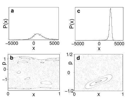
FIG. 1.: (a) Spatial distribution $P(x)$ of a continuously driven system [8] after $20,000$ time periods showing the directed transport in a Hamiltonian ratchet. Initially, $10^{4}$ trajectories were started at random on the line $p=0$, $x\in[0,1)$ in the chaotic sea. (b) Poincaré section $p$ vs $x$ of a unit cell at integer times showing the main chaotic sea, the upper and lower limiting KAM-tori, and the major embedded regular islands. (c,d) As (a,b), but for the kicked Hamiltonian (4) showing a much more pronounced directed transport.

We consider a Hamiltonian of the form $H(x,p,t)=T(p)+V(x,t)$, where $T(p)$ is the kinetic energy. The force $-V^{\prime}$ is periodic in space and time, $V^{\prime}(x+1,t)=V^{\prime}(x,t+1)=V^{\prime}(x,t)$, and has zero mean $\int_{0}^{1}{\rm d}t\,\int_{0}^{1}{\rm d}x\,V^{\prime}(x,t)=0$. Usually directed transport is demonstrated by following selected trajectories over very long times [5, 6] or an ensemble of trajectories which generates spatial distributions as shown in Fig. 1a,c. While this is easily implemented numerically, it gives no clue about the origin of the transport (but see Ref. [9]). Instead, we shall exploit the periodicity of the dynamics with respect to space and time and analyze transport in terms of the invariant sets of phase space, reduced to the spatio-temporal unit cell $x,t\in[0,1)$. For any finite invariant set $M$ we define ballistic transport as phase-space volume times average velocity expressed as

$$\tau_{M}=\int_{0}^{1}{\rm d}t\,\int_{0}^{1}{{\rm d}x}\,\int_{-\infty}^{+\infty}{\rm d}p\,\chi_{M}(x,p,t)\,{\partial H\over\partial p}\,,$$ (1)

where $\chi_{M}$ is the characteristic function of $M$. Transport is additive for the union of two or more disjunct invariant sets, i.e., for $M=\bigcup_{i}M_{i}$, with $M_{i}\cap M_{j}=\emptyset$ for all $i\neq j$, we have

$$\tau_{M}=\sum_{i}\tau_{M_{i}}\,.$$ (2)

This sum rule for Hamiltonian transport has far-reaching consequences to be discussed in the following.

For a generic Hamiltonian system, phase space is mixed and comprises an infinite number of minimal invariant sets of different types. For the sake of definiteness we will restrict the following discussion to the most interesting case of a chaotic region containing embedded regular islands (Fig. 1b). In any of these invariant sets the time-averaged velocity $v_{i}$ is the same for almost all initial conditions (assuming ergodicity for chaotic components). Hence, for a chaotic region, $\tau_{\rm ch}=A_{\rm ch}\,v_{\rm ch}$ with $A_{\rm ch}$ denoting its area in a stroboscopic Poincaré section. For an embedded island we have $\tau_{i}=A_{i}\,v_{i}$ where $A_{i}$ includes the areas of the narrow chaotic layers inside the island and of the infinite hierarchy of island chains surrounding it because all these invariant sets share the same mean velocity. This velocity $v_{i}$ is identical to the rational winding number $w_{i}=x_{i}/t_{i}$ of the stable fixed point at the center of the island. In extended phase space, this corresponds to a shift of the island by $x_{i}$ spatial after $t_{i}$ time periods. Typically, the chaotic set is bounded from above and below by two non-contractible KAM-tori $p_{a,b}(x,t)$ enclosing the spatial unit cell. Treating the phase-space region in between as the global invariant set $M$ appearing on the l.h.s. of Eq. (2), its transport $\tau_{M}$ is obtained from Eq. (1) as $\langle T\rangle_{{a}}-\langle T\rangle_{{b}}$ with $\langle T\rangle_{{a,b}}=\int_{0}^{1}{\rm d}t\,\int_{0}^{1}{\rm d}x\,T(p_{a,b}(x,t))$ denoting averages of the kinetic energy over the tori. Using the sum rule (2) we can now express transport of the chaotic region in terms of its adjoining regular components (KAM-tori and islands) as

$$A_{\rm ch}v_{\rm ch}=\langle T\rangle_{{a}}-\langle T\rangle_{{b}}-\sum_{i}A_{i}\,w_{i}\,.$$ (3)

This is our main result on classical transport in Hamiltonian ratchets. Not only does Eq. (3) provide an efficient method to determine the chaotic drift velocity, it also expresses the simple principle generating directed ballistic motion: Decomposing phase space into different invariant sets, these will in general have average velocities different from each other and also different from zero but related by the sum rule (2). Therefore a necessary condition for directed chaotic transport in Hamiltonian ratchets is a mixed phase space.

Lévy flights [10] are a characteristic feature of chaotic motion in a generic mixed phase space and indeed they were observed in Hamiltonian ratchets [5, 6]. They reflect the slow exchange between subsets of a chaotic region, separated by leaky barriers [10]. As these subsets are not invariant, their contributions to Eq. (2) are contained in the contribution of the chaotic invariant set. Lévy flights lead to power-law tails in spatial distributions. For example, the asymmetric shapes of the peaks visible in Figs. 1a,c can be attributed to these tails. Notably, in Fig. 1c one clearly sees a mean transport to the right although the same data shows no indication of a power-law tail in this direction. We stress that the sum rule allows to predict the mean velocity of chaotic trajectories without any reference to such details of the chaotic dynamics. This suggests that Lévy flights are not a necessary element of the mechanism of chaotic transport in Hamiltonian ratchets.

In Ref. [5] it was shown that a necessary condition for directed transport is the breaking of all symmetries which to each trajectory generate a countermoving partner. For a chaotic set invariant under such a symmetry, this is in agreement with Eq. (3) because then the r.h.s. vanishes identically. However, chaotic sets can also occur as symmetry-related pairs transporting in opposite directions. Moreover, if phase space cannot be decomposed into invariant subsets, e.g., for an ergodic system, there cannot be transport even with all symmetries broken.

Up to now we have only considered transport of invariant sets of the unit cell. For an arbitrary initial distribution transport is determined by projection onto these invariant sets [11]. Therefore, the location of an initial distribution within an invariant set is irrelevant. This applies also to the location within the temporal unit cell, i.e., to the question of phase dependence discussed in [12]. In particular, in case that the plane $p=0$, $0\leq x,t\leq 1$ is completely within the chaotic invariant set, any initial condition restricted to this plane will result in the same average transport. We now understand how a Hamiltonian ratchet makes particles initially at rest ($p=0$) move with a predetermined mean velocity as, e.g., in Fig. 1a.

We have checked Eq. (3) numerically for a continuously driven system [8]. We determined the areas $A_{i}$ and winding numbers $w_{i}$ for the regular islands shown in the Poincaré section of Fig. 1b as well as $\langle T_{a}\rangle$ and $\langle T_{b}\rangle$ for the limiting KAM-tori, yielding $v_{\rm ch}=0.092\pm 0.011$. The error estimate includes the uncertainty in the location of the bounding KAM-tori and the contribution from neglected small islands. The result is in agreement with the value $v_{\rm ch}=0.082\pm 0.002$ determined with much more computational effort from the spatial distribution of $10^{4}$ trajectories, started with $p=0$ (Fig. 1a).

As a minimal model for directed chaotic transport in Hamiltonian ratchets, we propose a kicked Hamiltonian

$$H(x,p,t)=T(p)+V(x)\,\sum_{n}\delta(t-n).$$ (4)

It reduces the dynamics to a map for position and momentum $x_{n+1}=x_{n}+T^{\prime}(p_{n})$, $p_{n+1}=p_{n}-V^{\prime}(x_{n+1})$, just after the kick. As an example we take a symmetric potential $V(x)=(x\,{\rm mod}\,1\,-1/2)^{2}/2$ and an asymmetric kinetic energy $T(p)=|p|+3\sin(2\pi p)/(4\pi^{2})$. We consider the dynamics on a cylinder with transport along the $x$-axis and $p\in[-1/2,+1/2)$ being a periodic variable. Fig. 1d shows the Poincaré section for one unit cell. There are only two major invariant sets—a chaotic sea and a regular island centered around a periodic orbit with winding number $w_{\rm reg}=-1$. According to Eq. (1), transport of the full phase space vanishes identically because of the periodic momentum variable. Applying the sum rule (2) the contributions to transport from the two invariant sets cancel exactly,

$$A_{\rm ch}\,v_{\rm ch}+A_{\rm reg}\,w_{\rm reg}=0\,.$$ (5)

We find the transport velocity of the chaotic component as $v_{\rm ch}=f_{\rm reg}/(1-f_{\rm reg})$, where $f_{\rm reg}=A_{\rm reg}/(A_{\rm reg}+A_{\rm ch})$ denotes the relative area of the regular island. From Fig. 1d, $f_{\rm reg}=0.117\pm 0.001$, thus $v_{\rm ch}=0.133\pm 0.001$ in agreement with $v_{\rm ch}=0.1344\pm 0.0003$ from the spatial distribution of Fig. 1c.

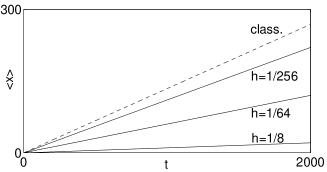
FIG. 2.: Mean position vs time for a wavepacket in system (4) initialized as the momentum eigenstate with $p=0$ for various values of $h$ (full lines). For decreasing $h$ the classical prediction $v_{\rm ch}\,t$ (dashed line) is approached.

In order to extend our concept of directed transport in Hamiltonian systems to quantum ratchets, we first demonstrate by a numerical example that quantum Hamiltonian ratchets can work. Fig. 2 shows that the average velocity of a wavepacket initialized in the chaotic sea varies between $0$ for large and the classical value $v_{\rm ch}$ for small values of $\hbar$. We explain this behavior in the following.

In analogy with our approach to classical transport, we consider the invariants of the quantum dynamics, the stationary states of the time-evolution operator over one period, i.e., $\hat{U}={\rm e}^{-{\rm i}\hat{V}/\hbar}{\rm e}^{-{\rm i}\hat{T}/\hbar}$ for the kicked Hamiltonian Eq. (4). They satisfy $\hat{U}|\phi_{\alpha,k}\rangle=\exp(-2\pi{\rm i}\epsilon_{\alpha}(k))\,|\phi_{\alpha,k}\rangle$, with the quasienergy $\epsilon_{\alpha}(k)\in[0,1)$ [13]. Similarly, spatial periodicity implies $\phi_{\alpha,k}(x+1,t)=\exp(2\pi{\rm i}k)\,\phi_{\alpha,k}(x,t)$ with quasimomentum $k\in[0,1)$ where $h$ is chosen rational for systems periodic in $p$. Quantum transport is related to the expectation values in the stationary states $\overline{v}_{\alpha,k}\equiv\langle\langle{\phi_{\alpha,k}|\hat{v}|\phi_{\alpha,k}}\rangle\rangle$ of the velocity operator $\hat{v}=\hat{T}^{\prime}(\hat{p})$, where $\langle\langle\cdot\rangle\rangle=\int_{0}^{1}{\rm d}x\int_{0}^{1}{\rm d}t(\cdot)$. Using a generalization of the Hellman-Feynman theorem to time-periodic systems [13], we express velocities by band slopes as

$$\overline{v}_{\alpha,k}={\rm d}\epsilon_{\alpha}(k)/{\rm d}k\,.$$ (6)

This allows to discuss quantum transport in terms of spectral properties. Examples for quasienergy band spectra are shown in Fig. 3 together with the corresponding velocity distributions. The semiclassical regime is characterized by the existence of two different types of bands and corresponding eigenstates [14, 15]: Bands pertaining to regular states appear as straight lines in the spectrum, while the chaotic bands show oscillations and wide avoided crossings among themselves. Associating the terms chaotic and regular with the bands is supported by the Husimi representations of the corresponding eigenfunctions (insets in Fig. 3a). The new aspect introduced into this picture by directed chaotic transport is the overall slope of the chaotic bands.

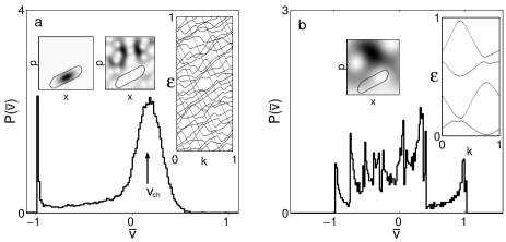
FIG. 3.: Distribution of quantum velocities $\overline{v}$ obtained according to Eq. (6) for (a) $h=1/128$ and (b) $h=1/4$. The right insets show band spectra for $h=1/32$ and $h=1/4$, respectively. The smaller insets are Husimi representations of characteristic wave functions together with the border of the classical regular island. In (a) the regular and the chaotic wave functions can be associated with the two peaks of $P(\overline{v})$ centered around $v_{\rm reg}=-1$ and $v_{\rm ch}$.

Only on a coarse quasienergy scale, the two sets of bands appear to cross. On a sufficiently fine scale, all crossings are avoided. Consequently the actual bands change their character between regular and chaotic at each of the narrow crossings and have no overall slope. Switching from the latter (“adiabatic”) to the former (“diabatic”) viewpoint is a well-controlled procedure [14]. Formally, this behavior of the bands can be described in terms of their winding number (average slope) with respect to the periodic $(\epsilon,k)$-space: In the adiabatic as well as in the diabatic case, all quasienergy bands must close after an integer number of periods in the $\epsilon$ and $k$ directions, so that their winding number $\overline{w}$ must be rational. Clearly, in the adiabatic case, all winding numbers are zero. Going from the adiabatic to the diabatic case amounts to a mere reconnection of bands at the crossings, preserving the sum of winding numbers. Thus it must be zero also in the diabatic representation,

$$\sum_{\alpha}\overline{w}_{\alpha}^{\rm(ch)}+\sum_{\alpha}\overline{w}_{\alpha}^{\rm(reg)}=0\,.$$ (7)

This is the quantum-mechanical analogue of the classical sum rule (5). Because of the localization of the regular states on tori inside the regular island, the winding number of the regular bands in $(\epsilon,k)$-space is in the semiclassical limit identical to the winding number in $(x,t)$-space of the central periodic orbit, i.e., $\overline{w}_{\alpha}^{\rm(reg)}=w_{\rm reg}$. Moreover, in this limit, the fractions of regular and chaotic bands correspond to the relative phase-space volumes $f_{\rm reg}$ and $1-f_{\rm reg}$, respectively. We therefore obtain from Eq. (7) the mean slope of the chaotic bands, $\overline{w}^{\rm(ch)}=f_{\rm reg}/(1-f_{\rm reg})=v_{\rm ch}$, as the classical drift velocity. This is confirmed in Fig. 3a.

The asymptotic quantum transport velocity for a given initial wavepacket $|\psi\rangle$ is an average of band slopes weighted with the overlaps $|\langle\psi|\phi_{\alpha,k}\rangle|^{2}$. We can now explain our observations in Fig. 2: For $\hbar\ll A_{\rm reg}$, an initial wavepacket prepared in the chaotic region of a single unit cell of the extended system is a superposition of chaotic eigenfunctions from the entire band spectrum. Consequently, its drift velocity is given by the mean slope of the chaotic bands and thus by the classical value $v_{\rm ch}$. In contrast, for $\hbar\gg A_{\rm reg}$, there are no states restricted to the regular or the chaotic set and hence quantum transport does not correspond to classical transport in this regime.

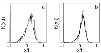
FIG. 4.: Form factor $K(x,t)$ for $h=1/128$ (thick line) at (a) $t=30$ and (b) $t=111$, the Heisenberg time of the chaotic component. The two distinct peaks centered around $v_{\rm reg}$ and $v_{\rm ch}$ are the fingerprints of directed transport. The time-dependent width of the chaotic peak follows the classical distribution $P^{\rm(ch)}(x,t)$ of chaotic trajectories (thin line).

Our analysis based on the winding numbers can be applied to predict the mean quantum transport in the semiclassical regime from the classical value. The band spectra, however, encode more detailed information about quantum transport. It can be extracted by a double Fourier transform $\epsilon\to t$, $k\to x$ (discrete position in units of the spatial period) and subsequent squaring of the spectral density, translating two-point correlations in the bands into the entire time evolution of the spatial distribution on the scale of the spatial period. A formal definition of the resulting generalized form factor $K(x,t)$ and further details are found in [16]. A semiclassical theory for the form factor in Hamiltonian ratchets, which will be published elsewhere, requires to account for the simultaneous presence of regular and chaotic regions in phase space. It relates the form factor $K(x,t)$ to the respective contributions of these invariant sets to the classical spatio-temporal distribution $P(x,t)$ (Fig. 4).

We benefitted from discussions with S. Flach, P. Hänggi, M. Holthaus and O. Yevtushenko. MFO acknowledges financial support from the Volkswagen foundation. TD thanks for the hospitality enjoyed during stays at the MPI für Physik komplexer Systeme, Dresden, and the MPI für Strömungsforschung, Göttingen, generously financed by the MPG.

REFERENCES

- [1] R. P. Feynman, R. B. Leighton, and M. Sands, The Feynman Lectures on Physics, Addison-Wesley, Reading, MA (1966), vol. 1, chap. 46.
- [2] F. Jülicher, A. Ajdari, and J. Prost, Rev. Mod. Phys. 69, 1269 (1997).
- [3] R. Bartussek, P. Hänggi, and J. G. Kissner, Europhys. Lett., 28, 459 (1994). P. Jung, J. G. Kissner, and P. Hänggi, Phys. Rev. Lett. 76, 3436 (1996).
- [4] J. L. Mateos, Phys. Rev. Lett. 84, 258 (2000).
- [5] S. Flach, O. Yevtushenko, and Y. Zolotaryuk, Phys. Rev. Lett. 84, 2358 (2000).
- [6] I. Goychuk and P. Hänggi in J. Freund and T. Pöschel (eds.) Lecture Notes on Physics, Vol. 557, pp. 7-20. Springer, Berlin (2000).
- [7] P. Reimann, M. Grifoni, and P. Hänggi, Phys. Rev. Lett. 79, 10 (1997); P. Reimann and P. Hänggi, Chaos 8, 629 (1998).
- [8] with and corresponding to the parameter set (3) of Fig. 1 in Ref. [5] where we have scaled the spatial and temporal period to 1.
- [9] S. Denisov and S. Flach, preprint nlin.CD/0104006.
- [10] T. Geisel in G. M. Zaslavsky (ed.) Lévy Flights and Related Phenomena in Physics. Springer, Berlin (1995).
- [11] T. Dittrich, R. Ketzmerick, M. F. Otto, and H. Schanz, Ann. Phys. (Leipzig) 9, 755 (2000).
- [12] O. Yevtushenko, S. Flach, and K. Richter, Phys. Rev. E 61, 7215 (2000).
- [13] H. Sambe, Phys. Rev. A 7, 2203 (1973).
- [14] A. R. Kolovsky, S. Miyazaki, and R. Graham, Phys. Rev. E 49, 70 (1994); S. Miyazaki and A. R. Kolovsky, Phys. Rev. E 50, 910 (1994).
- [15] In this work we neglect the existence of hierarchical states, but see R. Ketzmerick, L. Hufnagel, F. Steinbach, and M. Weiss, Phys. Rev. Lett. 85, 1214 (2000).
- [16] T. Dittrich, B. Mehlig, H. Schanz, and U. Smilansky, Phys. Rev. E 57, 359 (1998).