A geometric approach to singularity confinement and algebraic entropy

Abstract

A geometric approach to the equation found by Hietarinta and Viallet, which satisfies the singularity confinement criterion but exhibits chaotic behavior, is presented. It is shown that this equation can be lifted to an automorphism of a certain rational surface and can therefore be considered to be the action of an extended Weyl group of indefinite type. A method to calculate its algebraic entropy by using the theory of intersection numbers is presented.

1 Introduction

The singularity confinement method has been proposed by Grammaticos, Ramani and Papageorgiou [1] as a criterion for the integrability of (finite or infinite dimensional) discrete dynamical systems. The singularity confinement method demands that even if singularities would appear due to particular initial values, such singularities have to disappear after a finite number of iteration steps and that the information on the initial values can be recovered (hence the dynamical system has to be invertible).

However “counter examples” were found by Hietarinta and Viallet [2]. These mappings satisfy the singularity confinement criterion, but the orbits of their solutions exhibit chaotic behavior. The authors of [2] introduced the notion of algebraic entropy in order to test the degree of complexity of successive iterations. The algebraic entropy is defined as $s=\lim_{n\to\infty}\log(d_{n})/n$ where $d_{n}$ is the degree of $n$th iterate. This notion is linked with Arnold’s complexity, since the degree of a mapping gives the intersection number of the image of a line and a hyperplane. While the degree grows exponentially for a generic mapping, it was shown that it grows only in the polynomial order for a large class of integrable mappings [2, 3, 4, 5].

Many discrete Painlevé equations were found by Ramani, Grammaticos, Hietarinta, Jimbo and Sakai [6, 7] and have been extensively studied. Recently it was shown by Sakai [8] that all of these (from the point of view of symmetries) are obtained by studying rational surfaces in connection with the extended affine Weyl groups. Surfaces obtained by successive blow-ups [9] of ${\mathbb{P}}^{2}$ or ${\mathbb{P}}^{1}\times{\mathbb{P}}^{1}$ have been studied by several authors in the theory of birational mappings with invariants of finite ($=m$ in the case of ${\mathbb{P}}^{2}$ and $=m-1$ in the case of ${\mathbb{P}}^{1}\times{\mathbb{P}}^{1}$, $1\leq m\leq 8$) point sets in a rational surface connected to the Weyl groups [10, 11, 12]. Looijenga [13] and Sakai studied the case of $m=9$, in which case the birational mappings are connected with the extended affine Weyl groups and are obtained as Cremona transformations. Discrete Painlevé equations are recovered as particular cases.

Our aim in this letter is to characterize one of the mappings found by Hietarinta and Viallet from the point of view of the theory of rational surfaces. As its space of initial values, we obtain a rational surface associated with some root system of indefinite type. Conversely we recover the mapping from the surface and consequently obtain an extension of mapping to its non-autonomous version. By considering the intersection numbers of divisors, we also present a method to calculate the algebraic entropy of a mapping. It is shown that the degree of the mapping is given by the $n$th power of a matrix which is given by the action of the mapping on the Picard group.

2 Construction of the space of initial values by blow-ups

We consider the dynamical system written by the birational map $\varphi:{\mathbb{P}}^{1}\times{\mathbb{P}}^{1}\to{\mathbb{P}}^{1}\times{\mathbb{P}}^{1}$

$$(x_{n},y_{n})\mapsto(x_{n+1},y_{n+1})=(y_{n},-x_{n}+y_{n}+a/y_{n}^{2})$$ (1)

where $a\in{\mathbb{C}}$ is a nonzero constant. This equation was found by Hietarinta and Viallet [2] and we call it the HV eq.. To test the singularity confinement, let us assume $x_{0}\neq 0$ and $y_{0}=\epsilon$ where $|\epsilon|\ll 1$. With these initial values singularities appear at $n=1$ as $\epsilon\to 0$ and disappear at $n=4$. In this case the information on the initial values is hidden in the coefficients of higher degree $\epsilon$. However, taking suitable rational functions of $x_{n}$ and $y_{n}$ we can find the information of the initial values as finite values. The fact that the leading orders of $(x_{1}^{2}y_{1}-a)y_{1},~{}(x_{2}^{3}(y_{2}/x_{2}-1)^{2}-a)x_{2}$ and $(x_{3}y_{3}^{2}-a)x_{3}$ become $-ax_{0},-ax_{0}$ and $-ax_{0}$ actually suggests that the HV eq. can be lifted to an automorphism of a suitable rational surface. Although of course these rational functions are not uniquely determined.

Let the coordinates of ${\mathbb{P}}^{1}\times{\mathbb{P}}^{1}$ be $(x,y),(x,1/y),(1/x,y)$ and $(1/x,1/y)$ and let $x=\infty$ denote $1/x=0$. We consider the inverse mapping of the HV eq.

$$\varphi^{-1} : (x,y)\mapsto(\overline{x},\overline{y})=(-y+x+a/x^{2},x)$$ (2)

where $(\overline{x},\overline{y})$ means the image of $(x,y)$ by the mapping. This mapping has two indeterminate points: $(x,y)=(0,\infty),~{}(\infty,\infty)$. We denote blowing up at $(x,y)=(x_{0},y_{0})\in{\mathbb{C}}^{2}$: by

$$(x,y)\leftarrow(x-x_{0},(y-y_{0})/(x-x_{0}))\cup((x-x_{0})/(y-y_{0}),y-y_{0})$$ (3)

By blowing up at $(x,y)=(x_{0},y_{0})$, $(x-x_{0})/(y-y_{0})$ takes meaning at this point.

First we blow-up at $(x,y)=(0,\infty)$ , $(x,1/y)\leftarrow(x,1/xy)\cup(xy,1/y),$ and denote the obtained surface by $X_{0}$. Then $\varphi^{-1}$ is lifted to a rational mapping from $X_{0}$ to ${\mathbb{P}}^{1}\times{\mathbb{P}}^{1}$. For example, in the new coordinates $\varphi^{-1}$ is expressed as

$$(u_{1},v_{1}):=(x,1/xy) \mapsto (\overline{x},\overline{y})=((-u_{1}+u_{1}^{3}v_{1}+av_{1})/(u_{1}^{2}v_{1}),u_{1})$$

$$(u_{2},v_{2}):=(xy,1/y) \mapsto (\overline{x},\overline{y})=((-u_{2}^{2}v_{2}+u_{2}^{3}v_{2}^{3}+a)/(u_{2}^{2}v_{2}^{2}),u_{2}v_{2})$$

where $u_{1}=0$ and $v_{2}=0$. This maps the exceptional curve at $(x,y)=(0,\infty)$ almost to $(\overline{x},\overline{y})=(\infty,0)$ but has an indeterminate point on the exceptional curve: $(u_{1},v_{1})=(0,0).$ Hence we have to blow-up again at this point. In general it is known that, if there is a rational mapping $X\to Y$ where $X$ and $Y$ are smooth projective algebraic varieties, the procedure of blowing up can be completed in a finite number of steps, after which one obtains a smooth projective algebraic variety $X_{1}$ such that the rational mapping is lifted to a regular mapping from $X_{1}$ to $Y$ (theorem of the elimination of indeterminacy [9]).

Here we obtain the following sequence of blow-ups. (For simplicity we take only one coordinate of (3).)

$$(x,y) \smash{\mathop{\hbox to28.45274pt{\leftarrowfill}}\limits_{E_{5}}^{\mbox{at}~{}(0,\infty)}} \left(x,\frac{1}{xy}\right)\smash{\mathop{\hbox to28.45274pt{\leftarrowfill}}\limits_{E_{6}}^{(0,0)}}\left(x^{2}y,\frac{1}{xy}\right)$$

$$\smash{\mathop{\hbox to28.45274pt{\leftarrowfill}}\limits_{E_{7}}^{(a,0)}} \left(xy(x^{2}y-a),\frac{1}{xy}\right)\smash{\mathop{\hbox to28.45274pt{\leftarrowfill}}\limits_{E_{8}}^{(0,0)}}\left(x^{2}y^{2}(x^{2}y-a),\frac{1}{xy}\right)$$

$$(x,y) \smash{\mathop{\hbox to28.45274pt{\leftarrowfill}}\limits_{E_{9}}^{(\infty,\infty)}} \left(\frac{1}{x},\frac{x}{y}\right)\smash{\mathop{\hbox to28.45274pt{\leftarrowfill}}\limits_{E_{10}}^{(0,1)}}\left(\frac{1}{x},x(\frac{x}{y}-1)\right)$$

where the $E_{i}$ mean the total transforms generated by the blow-ups. Of course the sequence above is not unique, since there is freedom to choose the coordinates.

We have obtained a mapping from $X_{1}$ to ${\mathbb{P}}^{1}\times{\mathbb{P}}^{1}$ which is lifted from $\varphi^{-1}$. But our aim is to construct a rational surface $X$ such that $\varphi^{-1}$ is lifted to an automorphism of $X$. If it can be achieved, $X$ is considered to be the space of initial values in the sense of Okamoto [14], where a sequence of rational surfaces $X_{i}$ is (or $X_{i}$ themselves are) called the space of initial values for a sequence of rational mappings $\varphi_{i}$ if each $\varphi_{i}$ is lifted to an isomorphism from $X_{i}$ to $X_{i+1}$ for all $i$.

First we construct the rational surface $X_{2}$ such that $\varphi^{-1}$ is lifted to a regular mapping from $X_{2}$ to $X_{1}.$ For this purpose it is sufficient to eliminate the indeterminacy of mapping from $X_{1}$ to $X_{1}$. Consequently we obtain $X_{2}$ defined by the following sequence of blow-ups.

$$\left(\frac{1}{x},x(\frac{x}{y}-1)\right) \smash{\mathop{\hbox to28.45274pt{\leftarrowfill}}\limits_{E_{11}}^{(0,0)}} \left(\frac{1}{x^{2}(x/y-1)},x(\frac{x}{y}-1)\right)\smash{\mathop{\hbox to28.45274pt{\leftarrowfill}}\limits_{E_{12}}^{(0,0)}}\left(\frac{1}{x^{2}(x/y-1)},x^{3}(\frac{x}{y}-1)^{2}\right)$$

$$\smash{\mathop{\hbox to28.45274pt{\leftarrowfill}}\limits_{E_{13}}^{(0,a)}} \left(\frac{1}{x^{2}(x/y-1)},x^{2}(\frac{x}{y}-1)(x^{3}(\frac{x}{y}-1)^{2}-a)\right)$$

$$\smash{\mathop{\hbox to28.45274pt{\leftarrowfill}}\limits_{E_{14}}^{(0,0)}} \left(\frac{1}{x^{2}(x/y-1)},x^{4}(\frac{x}{y}-1)^{2}(x^{3}(\frac{x}{y}-1)^{2}-a)\right)$$

Next eliminating the indeterminacy of mapping from $X_{2}$ to $X_{2}$, we obtain $X_{3}$ defined by the following sequence of blow-ups.

$$(x,y) \smash{\mathop{\hbox to28.45274pt{\leftarrowfill}}\limits_{E_{1}}^{(\infty,0)}} \left(\frac{1}{xy},y\right)\smash{\mathop{\hbox to28.45274pt{\leftarrowfill}}\limits_{E_{2}}^{(0,0)}}\left(\frac{1}{xy},xy^{2}\right)$$

$$\smash{\mathop{\hbox to28.45274pt{\leftarrowfill}}\limits_{E_{3}}^{(0,a)}} \left(\frac{1}{xy},xy(xy^{2}-a)\right)\smash{\mathop{\hbox to28.45274pt{\leftarrowfill}}\limits_{E_{4}}^{(0,0)}}\left(\frac{1}{xy},x^{2}y^{2}(xy^{2}-a)\right)$$

Here, it can be shown that the mapping from $X_{3}$ to $X_{3}$ which is lifted from $\varphi^{-1}$ does not have any indeterminate points and has an inverse (the mapping lifted from $\varphi$). Hence we obtain the following theorem.

THEOREM 2.1

The HV eq. (1) can be lifted to an automorphism of $X(=X_{3})$.

3 Action on the Picard group

We denote the total transform of $x={\rm constant},$ (or $y={\rm constant}$) on $X$ by $H_{0}$ (or $H_{1}$ resp.) and the total transforms of the points subjected to blow-up by $E_{1},E_{2},\dots,E_{14}.$ It is known [9] that the Picard group of $X$, Pic($X$), is

$${\rm Pic}(X)={\mathbb{Z}}H_{0}+{\mathbb{Z}}H_{1}+{\mathbb{Z}}E_{1}+\cdots+{\mathbb{Z}}E_{14}$$

and the canonical divisor of $X$, $K_{X}$, is

$$K_{X}=-2H_{0}-2H_{1}+E_{1}+\cdots+E_{14}$$

It is also known that the intersection numbers of $H_{i}$ or $E_{k}$ and $H_{j}$ or $E_{l}$ are

$$H_{i}\cdot H_{j}=1-\delta_{i,j},~{}E_{k}\cdot E_{l}=-\delta_{k,l},~{}H_{i}\cdot E_{k}=0~{}$$ (4)

where $\delta_{i,j}$ is $1$ if $i=j$ and $0$ if $i\neq j.$

We denote the proper transforms, i.e. prime divisors, on $X$ by

$$H_{0},H_{1}(\mbox{ 0 curve (self-intersection number is 0}))$$

$$C_{0}:=E_{4},~{}C_{1}=E_{8},~{}C_{2}:=E_{14},~{}C_{3}:=H_{0}-E_{5},~{}C_{4}:=H_{1}-E_{1}~{}~{}(-1\mbox{ curve)}$$

$$D_{0}:=E_{1}-E_{2},~{}D_{1}:=E_{2}-E_{3},~{}D_{2}:=E_{3}-E_{4},~{}D_{3}:=E_{5}-E_{6},~{}D_{4}:=E_{6}-E_{7},~{}D_{5}:=E_{7}-E_{8},$$

$$D_{6}:=E_{9}-E_{10},~{}D_{7}:=E_{11}-E_{12},~{}D_{8}:=E_{12}-E_{13},~{}D_{9}:=E_{13}-E_{14}~{}~{}(-2\mbox{ curve)}$$

$$D_{10}:=H_{0}-E_{1}-E_{2}-E_{9},~{}D_{11}:=H_{1}-E_{5}-E_{6}-E_{9},~{}D_{12}:=E_{10}-E_{11}-E_{12}~{}~{}(-3\mbox{ curve)}$$

as in Fig.1. The intersection numbers of any pairs of divisors are given by linear combinations of these divisors.

The anti-canonical divisor $-K_{X}$ can be reduced to the distinct irreducible curves
$D_{0},D_{1},\cdots,D_{12}$ and the connection of $D_{i}$ are expressed by the Dynkin diagram:

The HV eq.(1) acts on curves as

$$\begin{array}[]{ll}&(D_{0},~{}D_{1},~{}D_{2},~{}D_{3},~{}D_{4},~{}D_{5},~{}D_{6},~{}D_{7},~{}D_{8},~{}D_{9},~{}D_{10},~{}D_{11},~{}D_{12},~{}C_{0},~{}C_{1},~{}C_{2})\\ \to&(D_{5},~{}D_{4},~{}D_{3},~{}D_{7},~{}D_{8},~{}D_{9},~{}D_{6},~{}D_{0},~{}D_{1},~{}D_{2},~{}D_{11},~{}D_{12},~{}D_{10},~{}C_{3},~{}C_{2},~{}C_{0})\end{array}$$ (7)

and $C_{4}\mapsto C_{1}$. Hence the HV eq. acts on Pic($X$) as

$$\left(\begin{array}[]{c}H_{0}\\ H_{1},~{}~{}E_{1},~{}~{}E_{2}\\ E_{3},~{}~{}E_{4},~{}~{}E_{5},~{}~{}E_{6}\\ E_{7},~{}~{}E_{8},~{}~{}E_{9},~{}~{}E_{10}\\ E_{11},~{}~{}E_{12},~{}~{}E_{13},~{}~{}E_{14}\end{array}\right)\to\left(\begin{array}[]{c}3H_{0}+H_{1}-E_{5}-E_{6}-E_{7}-E_{8}-E_{9}-E_{10}\\ H_{0},~{}~{}H_{0}-E_{8},~{}~{}H_{0}-E_{7}\\ H_{0}-E_{6},~{}~{}H_{0}-E_{5},~{}~{}E_{11},~{}~{}E_{12}\\ E_{13},~{}~{}E_{14},~{}~{}H_{0}-E_{10},~{}~{}H_{0}-E_{9}\\ E_{1},~{}~{}E_{2},~{}~{}E_{3},~{}~{}E_{4}\end{array}\right)$$ (18)

(this table means $\overline{H_{0}}=3H_{0}+H_{1}-E_{5}-E_{6}-E_{7}-E_{8}-E_{9}-E_{10},$ $\overline{H_{1}}=H_{0},$ $\overline{E_{1}}=H_{0}-E_{8}$ and so on.) and their linear combinations. As we will see in section 6, the action (18) provides a method to calculate the algebraic entropy of the HV eq.

4 An extended Weyl group acting on the Picard group

We shall decompose the action of the HV eq. on Pic($X$) as a product of actions of order two elements of what turns out to be an extended Weyl group. Let us define the actions $\sigma_{1},\sigma_{2},w_{1},w_{2},w_{3}$ on Pic(X) as follows (See Fig.1). (For simplicity we did not write the invariant elements under each action.)

$$\begin{array}[]{lll}&\sigma_{1}:&\left(\begin{array}[]{c}H_{0},~{}~{}H_{1},~{}~{}E_{1},~{}~{}E_{2},~{}~{}E_{3}\\ E_{4},~{}~{}E_{5},~{}~{}E_{6},~{}~{}E_{7},~{}~{}E_{8}\end{array}\right)\to\left(\begin{array}[]{c}H_{1},~{}~{}H_{0},~{}~{}E_{5},~{}~{}E_{6},~{}~{}E_{7}\\ E_{8},~{}~{}E_{1},~{}~{}E_{2},~{}~{}E_{3},~{}~{}E_{4}\end{array}\right)\\ &\sigma_{2}:&\left(\begin{array}[]{c}H_{1},~{}~{}E_{1},~{}~{}E_{2}\\ E_{3},~{}~{}E_{4},~{}~{}E_{9},~{}~{}E_{10}\\ E_{11},~{}~{}E_{12}~{}~{}E_{13},~{}~{}E_{14}\end{array}\right)\to\left(\begin{array}[]{c}H_{0}+H_{1}-E_{9}-E_{10},~{}~{}E_{11},~{}~{}E_{12}\\ E_{13},~{}~{}E_{14},~{}~{}H_{0}-E_{10},~{}~{}H_{0}-E_{9}\\ E_{1},~{}~{}E_{2},~{}~{}E_{3},~{}~{}E_{4}\end{array}\right)\\ &w_{1}:&\left(\begin{array}[]{c}H_{0},\\ E_{1},~{}~{}E_{2},~{}~{}E_{3},~{}~{}E_{4}\end{array}\right)\to\left(\begin{array}[]{c}H_{0}+2H_{1}-E_{1}-E_{2}-E_{3}-E_{4}\\ H_{1}-E_{4},~{}~{}H_{1}-E_{3},~{}~{}H_{1}-E_{2},~{}~{}H_{1}-E_{1}\end{array}\right)\\ &w_{2}:&\left(\begin{array}[]{c}H_{1},\\ E_{5},~{}~{}E_{6},~{}~{}E_{7},~{}~{}E_{8}\end{array}\right)\to\left(\begin{array}[]{c}2H_{0}+H_{1}-E_{5}-E_{6}-E_{7}-E_{8}\\ H_{0}-E_{8},~{}~{}H_{0}-E_{7},~{}~{}H_{0}-E_{6},~{}~{}H_{0}-E_{5}\end{array}\right)\\ &w_{3}:&\left(\begin{array}[]{c}H_{0},~{}H_{1},~{}E_{9},~{}E_{10}\\ E_{11},~{}E_{12},~{}E_{13},~{}E_{14}\end{array}\right)\to\left(\begin{array}[]{c}H_{0}+\alpha_{3},~{}H_{1}+\alpha_{3},~{}E_{9}+\alpha_{3},~{}E_{10}+\alpha_{3}\\ E_{11}+\alpha_{3}^{1},~{}E_{12}+\alpha_{3}^{2},~{}E_{13}+\alpha_{3}^{2},~{}E_{14}+\alpha_{3}^{1}\end{array}\right)\end{array}$$ (46)

where $\alpha_{3}^{1}=H_{0}+H_{1}-E_{9}-E_{10}-E_{11}-E_{14}$, $\alpha_{3}^{2}=H_{0}+H_{1}-E_{9}-E_{10}-E_{12}-E_{13}$ and $\alpha_{3}=\alpha_{3}^{1}+\alpha_{3}^{2}$.

Then (18) becomes $w_{2}\circ\sigma_{2}\circ\sigma_{1}$ and the following relations hold.

$$w_{i}^{2}=\sigma_{j}^{2}=1,~{}~{}(\sigma_{1}\sigma_{2})^{3}=1,$$

$$\sigma_{1}w_{1}=w_{2}\sigma_{1},~{}~{}\sigma_{1}w_{2}=w_{1}\sigma_{1},~{}~{}\sigma_{1}w_{3}=w_{3}\sigma_{1}$$ (47)

$$\sigma_{2}w_{1}=w_{3}\sigma_{2},~{}~{}\sigma_{2}w_{2}=w_{2}\sigma_{2},~{}~{}\sigma_{2}w_{3}=w_{1}\sigma_{2}$$

The basis of the root system

Let us define $\alpha_{1},\alpha_{2}$ $\alpha_{3}\in{\rm Pic}(X)$ as

$$\alpha_{1} = 2H_{1}-E_{1}-E_{2}-E_{3}-E_{4},$$

$$\alpha_{2} = 2H_{0}-E_{5}-E_{6}-E_{7}-E_{8},$$ (48)

$$\alpha_{3} = 2H_{0}+2H_{1}-2E_{9}-2E_{10}-E_{11}-E_{12}-E_{13}-E_{14}$$

It is satisfied that $\alpha_{i}\cdot D_{j}=0$ for all $j$. The actions of $\sigma_{j}$ and $w_{k}$ are

$$\sigma_{j}(\alpha_{i})\mbox{ and }w_{k}(\alpha_{i})$$

$$\begin{array}[]{|c|c|c|c|c|c|}\hline\cr&\sigma_{1}&\sigma_{2}&w_{1}&w_{2}&w_{3}\\ \hline\cr\alpha_{1}\mapsto&\alpha_{2}&\alpha_{3}&-\alpha_{1}&\alpha_{1}+2\alpha_{2}&\alpha_{1}+2\alpha_{3}\\ \hline\cr\alpha_{2}\mapsto&\alpha_{1}&\alpha_{2}&\alpha_{2}+2\alpha_{1}&-\alpha_{2}&\alpha_{2}+2\alpha_{3}\\ \hline\cr\alpha_{3}\mapsto&\alpha_{3}&\alpha_{1}&\alpha_{3}+2\alpha_{1}&\alpha_{3}+2\alpha_{2}&-\alpha_{3}\\ \hline\cr\end{array}$$ (53)

The action of $w_{i}$ can be written in the form $w_{i}(\alpha_{j})=\alpha_{j}-c_{ij}\alpha_{i}$ where $c_{ij}=2(\alpha_{i}\cdot\alpha_{j})/(\alpha_{i}\cdot\alpha_{i})$. Its Cartan matrix and Dynkin diagram are of the indefinite type $H_{71}^{(3)}$ [15]:

$$\left[\begin{array}[]{rrr}2&-2&-2\\ -2&2&-2\\ -2&-2&2\end{array}\right]\quad \alpha_{1} \alpha_{2} \alpha_{3}$$ and (57)

Hence it is seen [16] that the group of actions on Pic($X$) generated by ${w_{i}}$ and $\sigma_{i}$ coincides with the extended (including the full automorphism group of the Dynkin diagram) Weyl group of an indefinite type generated by

$$<w_{1},w_{2},w_{3},\sigma_{1},\sigma_{2}>$$ (58)

and the fundamental relations (47). From this fact we have the following theorem.

THEOREM 4.1

The HV eq. as the action of $w_{2}\sigma_{2}\sigma_{1}$ on Pic($X$) does not commute with any element of the group generated by $w_{i}$ and $\sigma_{i}$ except $(w_{2}\sigma_{2}\sigma_{1})^{m}$.

5 The inverse problem

A birational mapping on a rational surface is called a Cremona transformation. One method for obtaining a Cremona transformation (which exchanges a certain pair of exceptional curves) is to interchange the blow down structures. Following this method, we can construct the Cremona transformations which yield the extended Weyl group (58) and thereby recover the HV eq. from its action on Pic($X$).

These Cremona transformations are lifted to automorphisms of Pic($X$) but do not have to be lifted to automorphisms of $X$ itself, i.e. the blow-up points can be changed without however changing the intersection numbers (we consider isomorphisms from $X$ to $X^{\prime}$, where $X$ and $X^{\prime}$ may have different blow-up points). In order to do this, one has to consider not only autonomous but also non-autonomous mappings. By $a_{0},a_{1},a_{2},a_{3},a_{4},a_{5},a_{6},a_{7}$, we denote the point where each $E_{10},E_{3},E_{4},E_{7},E_{8},E_{11},E_{13},E_{14}$ is generated by the blow-up (or its value of the coordinate).

Consequently, it can been seen that $w_{2}$ is written as $w_{2}=t\circ w_{2}^{\prime}$, where $w_{2}^{\prime}:(x,y)\mapsto(x,y-a_{3}/x^{2}-a_{4}/(a_{3}x))$, and $t$ is a certain automorphism of ${\mathbb{P}}^{1}\times{\mathbb{P}}^{1}.$ By taking suitable $t$, we can assume that the points of $1,5,9$-th blow-up are fixed, $\overline{a_{0}}=a_{0}=1$ and $\overline{a_{5}}=a_{5}$. For the remaining points there are no such a priori requirements and there evolution under the present isomorphism should be calculated in detail. For example, under the above assumptions, $w_{2}$ can be seen to reduce to

$$w_{2}: (x,y;a_{1},a_{2},a_{3},a_{4},a_{5},a_{6},a_{7})\mapsto(\overline{x},\overline{y}~{};~{}\overline{a_{1}},\overline{a_{2}},\overline{a_{3}},\overline{a_{4}},\overline{a_{5}},\overline{a_{6}},\overline{a_{7}})$$ (59)

$$= \left(x,y-\frac{a_{3}}{x^{2}}-\frac{a_{4}}{a_{3}x}~{};~{}a_{1},a_{2}-\frac{2a_{1}a_{4}}{a_{3}},-a_{3},a_{4},a_{5},a_{6},a_{7}+\frac{2a_{4}a_{6}}{a_{3}}\right)$$

Here, in the calculation of the next iteration step we have to use $\overline{a_{3}}=-a_{3}$ instead of $a_{3}$.

Similarly $\sigma_{1}$ and $\sigma_{2}$ reduce to

$$\sigma_{1}: (x,y;a_{1},a_{2},a_{3},a_{4},a_{5},a_{6},a_{7})$$

$$\mapsto \left(-y,-x~{};~{}-a_{3},-a_{4},-a_{1},-a_{2},a_{5},-a_{6},a_{7}-4a_{5}^{2}a_{6}\right)$$

and

$$\sigma_{2}: (x,y;a_{1},a_{2},a_{3},a_{4},a_{5},a_{6},a_{7})$$

$$\mapsto \left(x,x-y-a_{5}~{};~{}a_{6},a_{7}-2a_{5}^{2}a_{6},-a_{3},a_{4},a_{5},a_{1},a_{2}+2a_{1}a_{5}^{2}\right)$$

Non-autonomous HV eq.

The composition $w_{2}\sigma_{2}\sigma_{1}$ reduces to

$$w_{2}\circ\sigma_{2}\circ\sigma_{1}:(x,y;a_{1},a_{2},a_{3},a_{4},a_{5},a_{6},a_{7})\mapsto(-y,x-y-a_{5}-\frac{a_{1}}{y^{2}}-\frac{a_{2}}{a_{1}y}~{};~{}$$

$$-a_{6},a_{7}-2a_{5}^{2}a_{6}-\frac{2a_{2}a_{6}}{a_{1}},-a_{1},-a_{2},a_{5},-a_{3},-a_{4}-2a_{3}a_{5}^{2}+\frac{2a_{2}a_{3}}{a_{1}})$$ (60)

Of course this mapping satisfies the singularity confinement criterion by construction and in the case of $a_{2}=a_{4}=a_{5}=a_{7}=0$ and $a_{1}=a_{3}=a_{6}=a$ it coincides with the HV eq.(1) except their signs. The difference between them comes from the assumption $\overline{a_{5}}=a_{5}$. Assuming $\overline{a_{5}}=-a_{5}$ by $w_{2},\sigma_{2}$ and $\sigma_{1}$, we have another form of (60)

$$w_{2}\circ\sigma_{2}\circ\sigma_{1}:(x,y;a_{1},a_{2},a_{3},a_{4},a_{5},a_{6},a_{7})\mapsto(y,-x+y+a_{5}+\frac{a_{1}}{y^{2}}+\frac{a_{2}}{a_{1}y}~{};~{}$$

$$a_{6},-a_{7}+2a_{5}^{2}a_{6}+\frac{2a_{2}a_{6}}{a_{1}},a_{1},a_{2},-a_{5},a_{3},a_{4}+2a_{3}a_{5}^{2}-\frac{2a_{2}a_{3}}{a_{1}})$$ (61)

Actually in the case of $a_{2}=a_{4}=a_{5}=a_{7}=0$ and $a_{1}=a_{3}=a_{6}=a$ it coincides with the HV eq.(1).

6 Algebraic entropy

In this section we consider the algebraic entropy which has been introduced by Hietarinta and Viallet to describe the complexity of rational mappings [2]. The degree of a rational function $P(x,y)=f(x,y)/g(x,y)$, where $f(x,y)$ and $g(x,y)$ are polynomials and $P(x,y)$ is irreducible, is defined by

$$\deg(P)=\max\{\deg f(x,y),\deg g(x,y)\}$$

where $\deg(x^{m}y^{n})=m+n$. The degree of the mapping $\varphi:(x,y)\mapsto(P(x,y),Q(x,y))$, where $P(x,y)$ and $Q(x,y)$ are rational functions, is defined by

$$\deg(\varphi)=\max\{\deg P(x,y),\deg Q(x,y)\}$$

The algebraic entropy of the map $\varphi:(x,y)\mapsto(P(x,y),Q(x,y))$ is defined by

$$\lim_{n\to\infty}\frac{1}{n}\log\deg(\varphi^{n})$$

if the limit exists. The definition of algebraic entropy of $\varphi$ coincides with the definition for the case where $\varphi$ is a rational mappings from ${\mathbb{P}}^{2}\to{\mathbb{P}}^{2}$. It is known [2] that the algebraic entropy of the HV eq. becomes $\log(3+\sqrt{5})/2$. We recover the algebraic entropy of the HV eq. by using the theory of intersection numbers.

Let us define the curve $D$ in $X$ as $y/x=c$, where $c\in{\mathbb{C}}$ is a nonzero constant. We denote the HV eq. by $\varphi$ and $(x_{n},y_{n})$ by $(P_{n}(x_{0},y_{0}),Q_{n}(x_{0},y_{0}))$. By the fundamental theorem of algebra, $\deg_{t}(P_{n}(t,ct))(=\deg(P_{n}(x,y))$ for $c\neq 1$) coincides with the intersection number of the curve $x=P_{n}(t,ct)$ and the curve $x=d$ in ${\mathbb{P}}^{1}\times{\mathbb{P}}^{1}$, where $\deg_{t}(P(t))$ is the degree of the rational function of one variable $P(t)$ and $d\in{\mathbb{C}}$ is a nonzero constant. It also coincides with the coefficient of $H_{1}$ as an element of Pic($X$). (Analogously for the intersection number of the curves related to $Q$ coincides with the coefficient of $H_{0}$.) The curve $D$ is expressed as $H_{0}+H_{1}-E_{9}$ in Pic($X$) if $c\neq 1$. Hence writing the coefficients of $H_{0}$ and $H_{1}$ of $\varphi^{n}(H_{0}+H_{1}-E_{9})$ as $h_{n}^{0},h_{n}^{1}$, we obtain the formula:

$$\deg(P_{n})=h_{n}^{1} \deg(Q_{n})=h_{n}^{0}$$

The action of $\varphi$ on Pic($X$) is given by (18). Hence the algebraic entropy of the HV eq. becomes $\lim_{n\to\infty}\frac{1}{n}\log\max\{h_{n}^{0},h_{n}^{1}\}$. In this case we have

$$\log\max\{|\mbox{ eigenvalues of }\varphi|\} = \log\frac{3+\sqrt{5}}{2}$$

The proof of the theorems contained in this letter as well as some other mappings, which satisfy the singularity confinement criterion but which have positive algebraic entropy, will be discussed in a forthcoming paper.

The author would like to thank H. Sakai, J. Satsuma, T. Tokihiro, A. Nobe, T. Tsuda, M. Eguchi and R. Willox for discussions and advice.

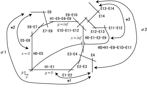
Figure 1:

References

• [1] Grammaticos B, Ramani A and Papageorgiou V 1991 Phys. Rev. Lett. 67 1825
• [2] Hietarinta J and Viallet C M 1998 Phys. Rev. Lett. 81 325
• [3] Arnold V I 1990 Bol. Soc. Bras. Mat. 21 1
• [4] Bellon M P and Viallet C M 1999 Comm. Math. Phys. 204 425
• [5] Ohta Y, Tamizhmani K M, Grammaticos B and Ramani A 1999 Phys. Lett. A 262 152
• [6] Ramani A, Grammaticos B, and Hietarinta J 1991 Phys. Rev. Lett. 67 1829
• [7] Jimbo M and Sakai H 1996 Lett.Math.Phys. 38 145
• [8] Sakai H 1999 Rational surfaces associated with affine root systems and geometry of the Painlevé equations Comm. Math. Phys.
at press webpage: http://www.kusm.kyoto-u.ac.jp/preprint/preprint99.html
• [9] Hartshorne R 1977 Algebraic geometry New York: Springer-Verlag
• [10] Cossec F and Dolgachev I 1988 Enrique’s surfaces I Boston: Birkhäuser
• [11] Dolgachev I 1983 Proc. Symp. Pure Math. 40 283
• [12] Dolgachev I 1988 Point sets in projective spaces and theta functions Astérisque 165 Soc. Math. de France
• [13] Looijenga E 1981 Annals of Math. 114 267
• [14] Okamoto K 1979 Japan J. Math. 5 1
• [15] Wan Z 1991 Kac-Moody algebra Singapore: World Scientific
• [16] Kac V 1990 Infinite dimensional lie algebras, 3rd ed., Cambridge: Cambridge University Press
Refer to caption