Analysis of a Parametrically Driven Pendulum

Abstract

We study in this paper the behavior of a periodically driven nonlinear mechanical system. Bifurcation diagrams are found which locate regions of quasiperiodic, periodic and chaotic behavior within the parameter space of the system. We also conduct a symbolic analysis of the model, which demonstrates that the symbolic dynamics of two-dimensional maps can be applied effectively to the study of ordinary differential equations in order to gain global knowledge about them.

I Introduction

In this paper we conduct an investigation of the behavior of a periodically driven nonlinear mechanical system. The system is of interest both from the point of view of the relatively rich structure it possesses and also because it is fairly easy to construct a mechanical model of it.

We begin with some standard techniques used to analyze such systems. Bifurcation diagrams are plotted which locate regions of quasiperiodic, periodic and chaotic behavior within the parameter space of the system. Dimensions of the attractor are calculated for different values of control parameters and compared with dimensions estimated from Lyapunov exponents. Numerical results obtained are in agreement with the Kaplan-Yorke conjecture. Multiple attractors are found in different regions in parameter space. The most interesting is the coexistence of a chaotic attractor and a limit cycle, which implies that initial conditions may determine whether the system will exhibit periodic or chaotic behavior. Boundaries of the basins of attraction appear to be smooth for high dissipation in the system, and they show fractal structure as the dissipation decreases. Creation and destruction of multiple attractors in this model is caused by tangent bifurcations and crisis phenomena. This illustrates how even a simple nonlinear mechanical system may exhibit fairly complex behavior and posses a variety of chaotic features.

We also conduct a symbolic analysis of the system. Symbolic dynamics provides almost the only rigorous approach to study the motion of dynamic systems. Such an analysis of one-dimensional maps on the interval is well understood mss ; h89 . For the simplest case of the unimodal map, a binary generating partition may be introduced by splitting the interval at the critical point. By assigning the letter $R$ or $L$ to a point of an orbit, depending whether it falls to the right or left side of the critical point, the orbit can be encoded with a symbolic sequence. The kneading sequence, which is the forward sequence of the critical value, determines all the admissible sequences of the map. By means of the kneading theory, all sequences are well ordered. The kneading sequence is the greatest. There is no allowed sequence which has a shifted sub-sequence greater than the kneading sequence.

The symbolic dynamics of the unimodal map can be extended to that of two-dimensional (2D) maps. Two much-studied 2D models are the Hénon map henon and its piecewise linear version, the Lozi map lozi ; zl94 . First of all, one needs to construct a ‘good’ binary partition for them. In Ref.gk85 , by considering all ‘primary’ homoclinic tangencies of the Hénon map, a method for determining a partition line was proposed. Once the binary partition is determined, any orbit may be associated with a doubly infinite symbolic sequence $S=\cdots s_{\overline{m}}\cdots s_{\overline{2}}s_{\overline{1}}\bullet s_{0}s_{1}\cdots s_{n}\cdots$ where $s_{0}$ indicates the code of the initial point. The forward sequence $\bullet s_{0}s_{1}\cdots s_{n}\cdots$ and backward sequence $\cdots s_{\overline{m}}\cdots s_{\overline{2}}s_{\overline{1}}\bullet$ correspond to the forward and backward orbits of the initial point, respectively. In Ref.cgp the ordering rules for forward and backward sequences were discussed, and by introducing a metric representation of sequences the symbolic plane was constructed. It was pointed out that every primary homoclinic tangency cuts out a rectangle of forbidden sequences in the symbolic plane. The rectangles so deleted build up a pruning front which is monotonic across half the symbolic plane. By generalizing stable and unstable manifolds of an unstable fixed or periodic point to forward and backward foliations of any point gu87 , homoclinic tangencies are generalized to tangencies between the two classes of foliations. In terms of the generalization, we can make symbolic analysis of the orbits not only in but also out of attractor, including transient orbits. The extension of symbolic dynamics of maps from 1D to 2D is made by decomposing a 2D map into two 1D maps based on forward and backward foliations. The coupling between the two 1D maps is described by the pruning front or the symbolic representation of the partition line. An attractor is associated with backward foliations.

It has been convincingly demonstrated that a properly constructed two-dimensional symbolic dynamics, being a coarse-grained description, provides a powerful tool to capture global, topological aspects of low-dimensional dissipative systems of ordinary differential equations (ODEs) lz95 ; lzh96 ; xzh95 ; zl95 ; lwz96 ; f95 ; fh96 ; zl97 ; hlz98 ; hao98 ; z9194 . Therefore, to have a further global understanding of the bifurcation and chaos “spectrum” in the system we have studied ito81 , i.e. the systematics of stable and unstable periodic orbits at varying and fixed parameters, the types of chaotic attractors, etc., we shall carry out a full analysis of symbolic dynamics for this mechanical model. Based on the primary tangencies between forward and backward foliations in the Poincaré section the appropriate partition of the phase space is made and three letters are used to describe the dynamics. From the ordering rules and metric representation of forward and backward sequences symbolic planes are constructed and the admissibility conditions for allowed sequences derived. Unstable allowed periodic orbits embedded in a chaotic attractor are predicted through symbolic analysis and verified numerically as well. In the parameter space period windows are located and the corresponding period words are determined according to the partitioning of phase portraits.

The paper is organized as follows. In section Section II a brief description of the mechanical system and a derivation of the equations of motion is given. In Section III chaos is detected, and regions of periodic, quasiperiodic and chaotic behavior are located within the parameter space. Lyapunov exponents and associated dimensions are calculated for certain attractors, and the Kaplan-Yorke conjecture is established. In section IV crisis phenomena and coexisting attractors are studied. We next turn to the symbolic dynamics of the module. In Section V, the global dynamical behavior of the system while parameters vary are shown in phase space, and the partition lines are determined from tangencies between forward and backward foliations in the Poincaré section. In Section VI by introducing a metric representation of forward and backward sequences according to their ordering rule the symbolic plane is constructed, and the admissibility condition of sequences is discussed. We then analyze the admissibility of periodic sequences based on a finite number of points on the partition lines, and give the numerical results of allowed periodic orbits in Section VII. We also locate the period windows for some range of parameters, assign words to the stable period orbits based on the partitioning of phase space, and discuss their ordering properties as parameters change in Section VIII. In Section IX we discuss some aspects of this model as used in a mechanical propulsion device. Finally, in Section X we present some conclusions.

II The Equation of Motion

Figure 1: Two gears and the rod

The system we study consists of two gears and a rod. The first one, the solar gear, has radius $R^{\prime}$, and is fixed so neither its center of mass can move nor can it rotate around its axis. The second, the planetary gear, is of radius $R$ and is attached to the first gear so when it rotates around its axis at the same time it goes around the fixed gear. We assume that the movable gear is powered by some device which keeps it moving with constant angular velocity $\omega_{d}$. When the planetary gear rotates for the angle $\phi$ around its axis it moves around solar gear for an angle $\phi^{\prime}$ (Fig. 1). The relation between two angles is

$$R^{\prime}\phi^{\prime}=R\phi$$ (1)

A uniformly dense rod of length $L$ is at one end joined to the fringe of movable gear. The rod can rotate around the joint, assumed without friction. Both gears and the rod lie in a horizontal plane so the potential energy of the system is constant during the motion. We choose a coordinate system with origin at the center of the fixed gear. The system has two degrees of freedom, and a convenient choice of coordinates are $\phi^{\prime}$, the angle that the second gear makes with $x$–axis, and $\vartheta$, the angle that the rod makes with the $x$–axis. Since the potential energy for the system is constant as well as the angular velocity of the planetary gear, the Lagrangian for the system is determined by the kinetic energy of the rod only. A general expression for the kinetic energy for the rigid body that moves in two dimensions is

$$T=\frac{1}{2}\int dm\,(\dot{x}+\dot{y})$$ (2)

We may express the position coordinates for the mass element $dm$ over coordinates $\phi$ and $\vartheta$ as

$$\begin{array}[]{c}x=(R^{\prime}+R)\cos\phi^{\prime}-R\cos(\phi^{\prime}+\phi)+l\cos\vartheta\\ y=(R^{\prime}+R)\sin\phi^{\prime}-R\sin(\phi^{\prime}+\phi)+l\sin\vartheta\end{array}$$ (3)

where $l$ is position of the mass element $dm$ at the rod. Deriving $x$ and $y$ over time and eliminating $\phi^{\prime}$ rather than $\phi$, using (1), we get:

$$\begin{array}[]{l}\dot{x}=-(1+r)R\dot{\phi}\sin r\phi+R(1+r)\dot{\phi}\sin\left[\left(1+r\right)\phi\right]-l\dot{\vartheta}\sin\vartheta\\ \dot{y}=(1+r)R\dot{\phi}\cos r\phi-R\dot{\phi}\left(1+r\right)\cos\left[\left(1+r\right)\phi\right]+l\dot{\vartheta}\cos\vartheta\end{array}$$ (4)

where $r=R/R^{\prime}$. Our initial assumption was that angular velocity of the planetary gear was constant $\dot{\phi}=\omega_{d}$. For simplicity, we will assume that initial condition is chosen so that $\phi=\omega_{d}t$. Substituting derivatives (4) into (2) and integrating over the whole rod, assuming its linear mass is constant, we get the kinetic energy, and therefore the Lagrangian, to be:

$$L=T=\frac{1}{2}I\dot{\vartheta}^{2}+\frac{1}{2}(1+r)mLR\omega_{d}\dot{\vartheta}\left\{\cos(\vartheta-r\phi)-\cos\left[\vartheta-\left(1+r\right)\phi\right]\right\}$$ (5)

Here $I$ is the moment of inertia of the rod, and we dropped terms that can be written as a total time derivative of some function and therefore do not contribute to the Lagrangian. Substituting this Lagrangian into the general expression for the Euler-Lagrange equations of motion of dissipative systems

$$\frac{d}{dt}\frac{\partial L}{\partial\dot{q}_{\alpha}}-\frac{\partial L}{\partial q_{\alpha}}=Q_{\alpha},~{}~{}~{}\alpha=1,...,s$$ (6)

and choosing $\vartheta$ and $\phi$ for coordinates we obtain the equation of motion to be

$$I\ddot{\vartheta}+\frac{1+r}{2}mLR\omega_{d}^{\,2}\left\{r\sin(\vartheta-r\phi)-(1+r)\sin\left[\vartheta-(1+r)\phi\right]\right\}=Q_{\vartheta}$$ (7)

where $Q_{\vartheta}$ is some friction force that acts upon the rod, and $I$ is its moment of inertia. If we assume that the friction, as is commonly done for a pendulum, has the simple form $Q_{\vartheta}=-\eta\dot{\vartheta}$ ($\eta>0$), we may write the equations of motion as

$$\ddot{\vartheta}+\frac{\eta}{I}\dot{\vartheta}+\omega_{0}^{\,2}\left\{\sin(\vartheta-r\phi)-\frac{1+r}{r}\sin[\vartheta-(1+r)\phi]\right\}=0,$$ (8)

where

$$\omega_{0}^{\,2}=r(1+r)\frac{mLR}{2I}\omega_{d}^{\,2}.$$ (9)

If we introduce now a new variable $\theta=\vartheta-r\phi$ we can bring the equations of motion to the arguably simpler form:

$$\ddot{\theta}+\frac{\eta}{I}\dot{\theta}+\omega_{0}^{\,2}\sin\theta=-\frac{\eta}{I}\omega_{d}+\frac{1+r}{r}\omega_{0}^{\,2}\sin(\theta-\phi).$$ (10)

This equation is nonlinear with a coupled term, and must be solved numerically. Therefore, for convenience we will write it in a dimensionless form by introducing the dimensionless time variable $\tau=\omega_{0}t$. Equation (10) then becomes

$$\ddot{\theta}+\frac{1}{Q}\dot{\theta}+\sin\theta=-\frac{ar}{Q}+\frac{1+r}{r}\sin(\theta-\phi),$$ (11)

where

$$a=\frac{\omega_{d}}{\omega_{0}}=\sqrt{\frac{2L}{3r(1+r)R}}$$

$$Q=\frac{\omega_{d}}{\eta}\sqrt{r\frac{1+r}{2}mlRI},$$ (12)

and

$$\phi=\omega_{d}t=a\tau.$$ (13)

Since we assume throughout this paper that $\omega_{D}$ is constant, the state of this system can be uniquely described in 3-dimensional phase space $(\theta,\dot{\theta},\phi)$. Furthermore, from the fact that $\phi$ depends linearly on time we may infer that trajectories in phase space will be “smooth” in the $\phi$ direction, and that all chaotic features, if any, can be observed in the Poincaré section $\phi=$ constant. In this way the problem of analyzing this three dimensional dynamical flow is reduced to the analysis of a two dimensional map.

Equation (11) has a similar form to that of the equation of motion for the driven pendulum, as well as to the Mathieu equation; however, there are some essential differences. The virtual drive frequency $a$ in the normalized equation (11) does not depend upon the drive frequency $\omega_{d}$ – the angular velocity of the moving gear – as it is constant which depends only on the dimensions of the rod and gears. On the other hand, the “quality” factor $Q$ is proportional to $\omega_{d}$, so a change of drive frequency will eventually appear as a change of dissipation in the system.

III Routes to Chaos

Figure 2: (a) Bifurcation graph showing broad chaotic region over segment of $Q$. $a=1.2$, $r=0.9$. (b) Corresponding change of the largest Lyapunov exponent.

For our system, we observe three characteristic regions in the parameter space – quasiperiodic, periodic and chaotic. In order to locate these regions we investigate the parameter space using bifurcation diagrams. Such diagrams show the evolution of the attractor for a dissipative system with a change of the system’s parameters. We choose to plot a projection of the Poincaré section $\phi=0$ on the $\dot{\theta}$ axis against the system’s parameter $Q$, while keeping other two parameters fixed. We repeat this procedure for various values of $a$ and $r$.

With the increase of $Q$ from zero on, the motion of the system is quasiperiodic, which is observed as a smeared region in the bifurcation graph. For certain value of $Q$ the motion suddenly becomes periodic, and with a further increase of the quality factor $Q$ the system reaches chaos through a sequence of period doublings. For the parameters $a,r<0.5$, the quasiperiodic region is relatively short, and chaos is found only in a narrow region of $Q$ values. The richest chaotic structure is found for the choice of parameters $a,r\sim 1$. Finally, for $a,r>1$ quasiperiodic motion becomes dominant over the range of $Q$, and periodic and possible chaotic behavior are found only in narrow isolated regions.

Figure 3: Power spectra for different values of quality factor $Q$: (a) $Q=0.2$ motion is quasiperiodic, (b) $Q=0.9$, motion is periodic with period one, (c) $Q=1.8$ and (d) $Q=6.5$, motion is chaotic. $\Theta(\omega)$ is the Fourier transform of $\dot{\theta}(t)$. The frequency on the $x$–axis is expressed in terms of the virtual drive frequency $a$.

Solid proof of chaos is the existence of at least one positive Lyapunov exponent. The spectrum of Lyapunov exponents gives us, besides qualitative information about a system’s behavior, also a quantitative measure of the system’s stability Ose68 ; Ben80 ; Shi79 ; Wol84 . Evolution of the Lyapunov exponent spectrum with a change of parameters gives us additional information about the system’s behavior to that from bifurcation graphs. Combined, these two methods are reliable tools for examining a system’s behavior and routes to chaos. Figure 2 gives a comparison of the bifurcation diagram and Lyapunov spectrum evolution for a range of $Q$. Since the system is represented in 3 dimensional space it is sufficient to determine only the largest Lyapunov exponent. The other two can be inferred from Haken’s theorem Hak83 , and the fact that the dissipation of the system is constant throughout phase space, so the sum of Lyapunov exponents must equal to its numerical value $\sum_{i}\lambda_{i}=1/Q$.

Figure 4: (a) Poincaré section of the quasiperiodic attractor is a smooth line. $a=1.2$, $r=0.9$, $Q=0.5$. (b) Poincaré section of the chaotic attractor reveals a kneading sequence. $Q=1.8$. (c) Higher dimensional chaotic attractor. $Q=6.5$.

A detailed description of the parameter space for this system is given in Ref.Pel00 . Here we illustrate its main features with a bifurcation diagram plotted for parameters $a=1.2$ and $0.9$ (Fig. 2a). The smeared region in the bifurcation diagram that is observed for the values $0<Q<0.6378\ldots$ corresponds to a quasiperiodic behavior of the system. Although it is generally possible to notice differences between chaotic and quasiperiodic regions in a bifurcation graph, it is necessary to employ other methods in order to have solid evidence of a system’s behavior.

Analysis of the power spectrum of the numerical solution is one of the methods that is particularly suitable for examining quasiperiodic motion. A power spectrum for $Q=0.5$ (Fig. 3a) shows that the motion of the system is a superposition of a finite number of harmonic modes, and therefore is not chaotic. The motion is not periodic though, since frequencies of harmonics are incommensurate, and the trajectory in phase space never retracts itself. The attractor for the system is a smooth 2-dimensional surface in phase space. The Poincaré section for $Q=0.5$ (Fig. 4a) indeed reveals smooth attractor.

For values of $0.7442\ldots<Q<0.9300\ldots$ it is clear from the bifurcation graph that the system’s behavior is periodic with period that is equal to the virtual drive period $2\pi/a$. This is also seen in the power spectrum for $Q=0.9$ in Figure  3b. With an increase of $Q$ over $1.2040\ldots$ the system becomes chaotic through a period doubling sequence. The smeared region in the bifurcation diagram indicates that the attractor for the system has a complex structure in that region of the parameter space. The power spectrum also shows complexity of the system’s behavior and indicates chaos in that region of parameter space. The power spectrum does not consist of a finite number of harmonics and their integer multiples any more, but is rather a broad band over the frequency axis (Figs. 3c and  3d). In order to obtain a solid evidence of chaos one has to show that at least one Lyapunov exponent for the system is positive in that region All97 . Indeed, Figure  2b shows that the largest Lyapunov exponent is positive in this region of parameter space, apart from windows of periodic behavior.

In particular, at $Q=1.8$ and $Q=6.5$ the largest Lyapunov exponents are found to be $\lambda_{1}=0.093\pm 0.005$ and $\lambda_{1}=0.106\pm 0.005$, respectively. The system’s attractors for these values of parameters (Figs. 4b and  4c) show characteristic stretching and folding pattern, indicating their fractal structure.

In the quasiperiodic region the attractor has dimension 2, as the motion is performed over a smooth surface, while the limit cycles have dimension 1. Since motion takes place in 3-dimensional phase space it is reasonable to expect that strange attractors have dimension between 2 and 3. We can use the fact that the attractor is always smooth in the $\phi$ direction, so in order to estimate its dimension we can estimate the dimension of its Poincaré section and obtain the attractor’s dimension simply by adding one to it.

$~{}~{}Q~{}~{}$	$D_{L}$	$D_{0}$	$D_{1}$	$D_{2}$
$0.5$	$2.000\pm 0.001$	$2.002\pm 0.003$	$2.007\pm 0.006$	$1.999\pm 0.002$
$1.8$	$2.14\pm 0.01$	$2.11\pm 0.01$	$2.044\pm 0.007$	$2.012\pm 0.003$
$6.5$	$2.41\pm 0.01$	$2.39\pm 0.01$	$2.389\pm 0.004$	$2.299\pm 0.001$

Table 1: Various dimensions of the attractors.

In order to estimate the dimension of an attractor lying in $n$–dimensional phase space, the attractor, first, has to be covered by a grid of $n$-dimensional hypercubes of size $\epsilon$, and then the probability of finding a point of the attractor in each hypercube $P_{i}$ has to be determined. The index $i$ here refers to a particular cube. In our case we consider a 2-dimensional Poincaré section, so the hypercubes are actually squares. A general expression for the dimensions of the $q^{\rm th}$-order is then given by:

$$D_{q}=\lim_{\epsilon\rightarrow 0}\frac{1}{q-1}\frac{\ln\sum_{i}P_{i}^{\,q}}{\ln\epsilon},$$ (14)

where the summation is over all hypercubes where $P_{i}>0$ Gra84 . The parameter $q$ ranges from $-\infty<q<\infty$, and for $q_{1}>q_{2}$ we have $D_{q_{1}}\leq D_{q_{2}}$. The most commonly used dimensions are $D_{0}$, $D_{1}$, and $D_{2}$, or the capacity, information, and correlation dimension, respectively. We will limit ourselves to estimating these three dimensions only.

On the other hand, the Lyapunov dimension of the attractor is defined as:

$$D_{L}=j+\frac{\lambda_{1}+\lambda_{2}+...+\lambda_{j}}{|\lambda_{j+1}|}$$ (15)

where $j$ is a largest integer for which $\lambda_{1}+\lambda_{2}+\ldots+\lambda_{j}\geq 0$. Kaplan and Yorke conjectured that the Lyapunov dimension represents an upper limit to the information dimension, i.e. $D_{L}\geq D_{1}$ Kap79 ; Led81 . It is to be expected though that numerical values of these four dimensions fall pretty close to each other Far83 .

We test this conjecture on our calculations for the quasiperiodic attractor (Fig. 4), and as expected we obtain the Lyapunov, capacity, information, and correlation dimensions to be equal 2, within the limits of uncertainty of our numerical methods. Furthermore, we can estimate these dimensions for the attractors in Figures  4b and  4c. Both chaotic attractors have noninteger dimensions (Table 1), confirming their fractal structure. In all three cases the inequality $D_{L}\geq D_{1}$ holds, suggesting that this system conforms Kaplan-Yorke conjecture.

IV Coexisting Attractors and Crisis

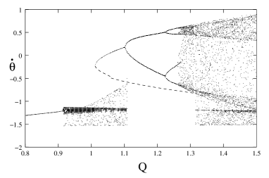
Figure 5: Bifurcation diagram indicating coexisting attractors. Dashed line shows unstable limit cycle.

Figure 6: Poincaré section of the chaotic attractor at the verge of crisis, shown within its basin of attraction in. White dots represent a stable, and black dots an unstable, limit cycle. $Q=1.8$.

An interesting feature of this system is that it often has periodic and chaotic attractors coexisting at the same point in parameter space. This means that the stability of this system may depend on the initial conditions – whether we choose it in the basin of periodic or chaotic attractor. Here we shall present two examples which illustrate the importance of understanding system’s dynamics in order to properly assess its stability.

The bifurcation diagram 5 shows that a tangent bifurcation Man79 occurs $Q=1.0105\ldots$, which creates a pair of stable and unstable limit cycles in the phase space, while a chaotic attractor still exists. Accordingly, the phase space splits into a basin of the stable limit cycle and a basin of the chaotic attractor. The boundary between the two basins appears to be a smooth curve (Fig. 6). With an increase of the control parameter $Q$ the basin of attraction for the limit cycle expands until the unstable limit cycle, which lies on its boundary, collides with the chaotic attractor. The chaotic attractor experiences a boundary crisis Gre83 and disappears along with its own basin. The basin of the limit cycle then suddenly expands, occupying the whole phase space. With a further increase of the control parameter the limit cycle evolves into a chaotic attractor through a sequence of period doublings. The newly created chaotic attractor expands in size as the parameter $Q$ increases, and eventually collides with the unstable limit cycle. The system comes to a crisis again, but since the unstable orbit is not at the basin boundary any more the crisis is internal, and the attractor suddenly expands its size Gre83 . This expanded attractor contains features of the chaotic attractor destroyed in the boundary crisis, indicating that information about the system’s behavior at lower values of $Q$ has “survived” the crisis.

Figure 7: Bifurcation diagram shows creation of coexisting attractors.

Figure 8: Three coexisting attractors. Period-three limit cycle (black points) and period-one limit cycle (white point) are enlarged for clarity. $Q=3.515$.

As we increase the control parameter $Q$ further, we observe another occurrence of coexisting attractors (Fig. 7). Tangent bifurcations at $Q=3.2398\ldots$ and $Q=3.4177\ldots$ create stable–unstable pairs of period–one and period–three orbits, respectively, so we have three coexisting attractors. Basin boundaries are now locally disconnected fractal curves McD85a , as shown in Figure  8. Basins of attraction are highly interwoven in this region, and for practical purposes it is difficult to determine initial conditions that would lead to a particular attractor. The newly created period–3 orbit quickly evolves to a chaotic attractor with an increase of the control parameter (Fig. 7), and disappears in a boundary crisis. Basins of attractions in Figures 6 and 8 are plotted using software package Dynamics 2 Nus .

V Partitioning of the Poincaré section

We now turn to a symbolic analysis of this model. For this, we shall choose convenient phase space $x=\theta/2\pi$, $y=\dot{x}$, and write the equations of motion in their nonautonomous form as

$$\begin{array}[]{l}\dot{x}=y,\\ \dot{y}=-y/Q+[-ar/Q-\sin(2\pi x)+(1+r)/r\sin(2\pi x-a\tau)]/(2\pi).\\ \end{array}$$ (16)

To show its richer properties in the phase and parameter spaces we fix $r=1.088$ and vary the values of $Q$ and $a$ in such a way that $a=0.8+0.3Q$. All Poincaré sections are constructed in $\phi=27\pi/64$ plane of phase space.

To observe the dynamics changes for varying $Q$ and $a$ we juxtapose the Poincaré sections (x, y) of attractors, the $x_{n}\rightarrow x_{n+1}$ first return map and the $\mu-\nu$ portraits where $\mu=1-(0.4+y)\cos(2\pi x)$ and $\nu=1-(0.4+y)\sin(2\pi x)$ at $Q=0.57,0.76,1.2577,1.68,{\rm and}~{}2.0$ from top to bottom in Fig. 9. Obviously, when $Q$ increases, 1) the portraits undergo the changes: 1D $\rightarrow$ 2D $\rightarrow$ 1D; 2) the return map $x_{n+1}-x_{n}$ shows: a subcritical circle map without any decreasing branch $\rightarrow$ the appearance of decreasing branches $\rightarrow$ a subcritical circle map; 3) the dynamical behavior exhibits: quasiperiodicity $\rightarrow$ chaos $\rightarrow$ quasiperiodicity.

Figure 9: Attractors shown in the $x-y,~{}x_{n}-x_{n+1},$ and $\mu-\nu$ planes at $Q=0.57,0.76,1.2577,1.68,{\rm and}~{}2.0$ from top to bottom for $r=1.088,{\rm and}~{}a=0.8+0.3Q.$

Figure 10: Attractor (dots) and forward foliations (dash curves) for $Q=0.57$.

The quasiperiodic attractor and forward foliations at $Q=0.57$ are shown in Fig. 10, from which one can see clearly that there is no any tangency between the attractor (part of backward foliations) and the forward foliations. As a matter of fact, when $Q$ increases to a value the tangencies begin to appear, and correspondingly one can obtain a critical circle or annular map $x_{n+1}-x_{n}$. If $Q$ keeps increasing, then the map would be supercritical. Finally there are no tangency and the map becomes subcritical again (see Fig. 9). This shows the close connection between the geometric properties (the tangencies) of an attractor and the dynamical behavior (quasiperiodicity and chaos) of a system.

Figure 11: The Poincaré map (dots) and forward foliations (dash curves) at $Q=0.76$. The primary partition lines $\bullet$B, $\bullet$C, and the pre-image $\bullet$A of $\bullet$B divide the attractor into three parts labeled by the letters L, R and N.

Figure 12: The $x_{n+1}-x_{n}$ first return map at $Q=0.76$.

Figure 13: The chaotic attractor (dots), forward foliations (dashed lines), and partition lines $\bullet$A, $\bullet$B, and $\bullet$C at $Q=1.2577$.

Figure 14: The $x_{n+1}-x_{n}$ first return map constructed from Fig. 13.

Figure 15: The $x^{\prime}_{n+1}-x^{\prime}_{n}$ swapped return map constructed from Fig. 14.

In Fig. 11 we show the attractor and two primary partition lines ($\bullet$B and $\bullet$C) on the background of the forward foliations (dash curves) for $Q=0.76$. The line marked with $\bullet$A is the pre-image of $\bullet$B. The areas in between these lines are labeled by $\bullet R$, $\bullet L$, and $\bullet N$. The corresponding first return map is plotted in Fig. 12. The three monotone segments in Fig. 12 are assigned the letters $L$, $R$, and $N$, in accordance with the two-dimensional partitions in Fig. 11.

A more interesting case is encountered at $Q=1.2577$. The attractor, three forward foliations passing tangencies and the primary partition lines are shown in Fig. 13, which manifestly exhibits two-dimensional feature. We also separately plot in Figs. 14 and 15 the $x_{n+1}-x_{n}$ first return map constructed from Fig. 13 by using the $x$ coordinates and its swapped form $x^{\prime}_{n+1}-x^{\prime}_{n}$ with

$$x^{\prime}=x+1-x_{B}\quad{\rm for}\quad x<x_{B},\quad{\rm or}\quad x^{\prime}=x-x_{B}\quad{\rm for}\quad x\geq x_{B},$$ (17)

where $x_{B}$ is the $x$ coordinate of the attractor tangency on the partition line $\bullet B$ in Fig. 13. Actually the partition lines $\bullet B$ and $\bullet A$ are not respectively parallel to the $x_{n+1}$-axis and $x_{n}$-axis in Figs. 14 and 15.

VI Ordering rule and admissibility condition

After the partition lines are determined, each point, or its orbit, may be encoded with a doubly infinite symbolic sequence consisting of the letters $R$, $L$ and $N$, say, $S=\cdots s_{\overline{m}}\cdots s_{\overline{2}}s_{\overline{1}}\bullet s_{1}s_{2}\cdots s_{n}\cdots$, where $s_{n}$ is the code for the $n$-th point of the forward orbit, and $s_{\overline{m}}$ the code for the $m$-th point of the backward orbit. The “present” position is indicated by a solid dot, which divides the doubly infinite sequence into two semi-infinite sequences, i.e., the backward sequence $\cdots s_{\overline{m}}\cdots s_{\overline{2}}s_{\overline{1}}\bullet$ and the forward sequence $\bullet s_{1}s_{2}\cdots s_{n}\cdots$.

A metric representation for symbolic sequences can be introduced by assigning numbers in $[0,1]$ to forward and backward sequences. We first assign an integer $\epsilon_{i}=-1$ or $1$ to the symbol $s_{i}$ when it is the letter $N$ or otherwise. Then we assign to the forward sequence $\bullet s_{1}s_{2}\cdots s_{n}\cdots$ the number

$$\alpha=\sum_{i=1}^{\infty}\mu_{i}3^{-i},\ \ \ \ \$$ (18)

where

$$\mu_{i}=\cases{0\cr 1\cr 2\cr}\quad{\rm for}\quad s_{i}=\cases{L\cr R\cr N\cr}\quad{\rm if}\quad\prod_{j=1}^{i-1}\epsilon_{j}=1,$$ (19)

or,

$$\mu_{i}=\cases{2\cr 1\cr 0\cr}\quad{\rm for}\quad s_{i}=\cases{L\cr R\cr N\cr}\quad{\rm if}\quad\prod_{j=1}^{i-1}\epsilon_{j}=-1.$$ (20)

Similarly, the $\beta$ assigned to the backward sequence $\cdots s_{\overline{m}}\cdots s_{\overline{2}}s_{\overline{1}}\bullet$ is defined by

$$\beta=\sum_{i=1}^{\infty}\nu_{\overline{i}}3^{-i},\ \ \ \ \$$ (21)

where

$$\nu_{\overline{i}}=\cases{0\cr 1\cr 2\cr}\quad{\rm for}\quad s_{i}=\cases{R\cr N\cr L\cr}\quad{\rm and}\quad\prod_{j=1}^{i-1}\epsilon_{\overline{j}}=1,$$ (22)

or

$$\nu_{\overline{i}}=\cases{2\cr 1\cr 0\cr}\quad{\rm for}\quad s_{i}=\cases{R\cr N\cr L\cr}\quad{\rm and}\quad\prod_{j=1}^{i-1}\epsilon_{\overline{j}}=-1.$$ (23)

According to the definition we have

$$\begin{array}[]{l}\alpha(\bullet NL^{\infty})=\beta(L^{\infty}\bullet)=1,\hskip 71.70107pt\alpha(\bullet L^{\infty})=\beta(R^{\infty}\bullet)=0,\\ \alpha(\bullet NNL^{\infty})=\alpha(\bullet RNL^{\infty})=2/3,\hskip 29.59067pt\beta(R^{\infty}L\bullet)=\beta(R^{\infty}N\bullet)=2/3,\\ \alpha(\bullet RL^{\infty})=\alpha(\bullet LNL^{\infty})=1/3,\hskip 42.67912pt\beta(L^{\infty}N\bullet)=\beta(L^{\infty}R\bullet)=1/3.\end{array}$$ (24)

In this representation a bi–infinite symbolic sequence with the present dot specified corresponds to a point in the unit square of the $\alpha-\beta$ plane, the so-called symbolic plane. In the plane, forward and backward foliations become vertical and horizontal lines, respectively. We may define the ordering rules of forward (or backward) sequences according to their $\alpha$ (or $\beta$) values. From Eqs. (18-8) we then have

$$\begin{array}[]{lr}\bullet EL\cdots<\bullet ER\cdots<\bullet EN\cdots,\hskip 28.45274pt\bullet OL\cdots>\bullet OR\cdots>\bullet ON\cdots,\\ \end{array}$$ (25)

and

$$\begin{array}[]{lr}\cdots RE\bullet<\cdots NE\bullet<\cdots LE\bullet,\hskip 28.45274pt\cdots RO\bullet>\cdots NO\bullet>\cdots LO\bullet,\\ \end{array}$$ (26)

where the finite strings $E$ and $O$ consist of letters $L$, $R$ and $N$ and contain an even and odd number of letter $N$, respectively. This ordering rule is similar to that for sequences of the dissipative standard map at some values of the parameters lzh96 .

Figure 16: The symbolic plane at $Q=0.76$. 10000 points of real orbits generated from the Poincaré map are also shown together with the FFZ in which no point falls.

Figure 17: The symbolic plane at $Q=1.2577$. Together with the FFZ, 10000 points representing real orbits are drawn. None of them falls inside the FFZ.

Figure 18: A blow-up of the symbolic plane Fig. 17 in the intervals $\alpha=[0.8794,0.87965]$ and $\beta=[0,0.65]$.

When foliations are well ordered, the geometry of a tangency places a restriction on allowed symbolic sequences. A point on the partition line $C\bullet$ (image of $\bullet C$) may symbolically be represented as $QC\bullet P$. The rectangle enclosed by the lines $QN\bullet$, $QR\bullet$, $\bullet P$, and $\bullet NL^{\infty}$ forms a forbidden zone (FZ) in the symbolic plane. Therefore, a symbolic sequence $IJ$ with $I\bullet$ between $QN\bullet$ and $QR\bullet$, and at the same time $\bullet J>\bullet P$ must be forbidden by the tangency $QC\bullet P$. In the symbolic plane the sequence $IJ$ corresponds to a point inside the forbidden zone of $QC\bullet P$. Similarly, $UB\bullet V$ stands for a tangency on the partition line $B\bullet$ (image of $\bullet B$). The lines $UL\bullet$, $UN\bullet$, $\bullet V$ and $\bullet L^{\infty}$ enclose a rectangle FZ in the symbolic plane. Any sequence $KT$ with $K\bullet$ between $UL\bullet$ and $UN\bullet$ while $\bullet T<\bullet V$ is forbidden by the $UB\bullet V$. Each tangency point on a partition line rules out a rectangle in the symbolic plane. The union of the forbidden rectangles, determined from one and the same partition line, forms the fundamental forbidden zone (FFZ), a boundary of which is the so-called pruning front. Consider a finite set of tangencies {$Q_{i}C\bullet P_{i}$} (or {$U_{j}B\bullet V_{j}$}). If the shift of a sequence $\cdots s_{k-2}s_{k-1}\bullet s_{k}s_{k+1}\cdots$ satisfies the condition that the backward sequence $\cdots s_{k-2}s_{k-1}\bullet$ is not between $Q_{i}N\bullet$ and $Q_{i}R\bullet$ (or $U_{j}N\bullet$ and $U_{j}L\bullet$) , and at the same time $\bullet P_{i}>\bullet s_{k}s_{k+1}\cdots$ (or $\bullet V_{j}<\bullet s_{k}s_{k+1}\cdots$) for some $i$ ($j$), then this shift is not forbidden by any tangencies of $C\bullet$ or $B\bullet$, owing to the property of well-ordering of foliations. Thus, we may say that the shift is allowed according to that tangency. A necessary and sufficient condition for a sequence to be allowed is that all of its shifts are allowed according to the two sets of tangencies. To check the admissibility condition, we consider again the two cases $Q=0.76$ and $Q=1.2577$, and draw $10000$ points representing real sequences generated from the Poincaré map together with the FFZ in the symbolic plane, as seen in Figs. 16 and 17. One can see that the FFZ indeed contains no point of allowed sequences. A blow-up of the right-hand side pruning front in Fig. 17 is displayed in Fig. 18. The structure means two-dimensional feature, related to the two tangent points in the upper part of attractor on the partition line $\bullet C$ (see Fig. 13). We shall use the two tangencies to make 2D analysis of periodic sequences later on (see T₃ and T₄ in the next section).

VII Unstable periodic orbit sequences

The attractor at $Q=0.76$ does not show much two–dimensional nature, so the reduction to symbolic dynamics of one-dimensional circle map may capture much of the essentials. We start from this simple case. The attractor resembles that of a one–dimensional circle map except for a segment with two sheets, one of which without the $N$ part ( see Figs. 11 and 12). From the two primary partition lines $\bullet C$ and $\bullet B$ in Fig. 11, we get the following sequences for attractor points:

$$\begin{array}[]{rc}{\rm T_{1}:}&\cdots NN\cdots NNAB\bullet LRRLNLNLNLRRRLLRRR\cdots,\\ {\rm T_{2}:}&\cdots NN\cdots NNLC\bullet RRLRLNLRRRLRLNRLNL\cdots.\\ \end{array}$$

In order to reduce the two-dimensional attractor to one-dimensional return map, we need to determine two kneading sequences $K_{B}$ and $K_{C}$. They are the forward sequences of ${\rm T_{1}}$ and ${\rm T_{2}}$, respectively.

$$\begin{array}[]{rcl}{\rm K_{B}}&=&LRRLNLNLNLRRRLLRRR\cdots,\\ {\rm K_{C}}&=&RRLRLNLRRRLRLNRLNL\cdots.\\ \end{array}$$ (27)

Compared with the original 2D map, the 1D circle map given by these ${\rm K_{B}}$ and ${\rm K_{C}}$ puts less constraints on allowed orbits. Since the attractor has only one sheet crossing each primary partition line nearly no difference between the 1D and 2D maps can be recognized if the sequences of short periodic orbits are concerned.

The knowledge of the two kneading sequences (27) determines everything in the symbolic dynamics of the circle map z9194 . For example, one may define a rotation number $W$, also called a winding number, for a symbolic sequence by counting the weight of letters $R$ and $N$ in the total number $n$ of all letters:

$$W=\lim_{n\rightarrow\infty}{\frac{1}{n}}{\rm(Number\,\,\,of\,\,\,R\,\,\,and\,\,\,N)}.$$ (28)

Chaotic regime is associated with the existence of a rotation interval, a closed interval in the parameter plane ito81 . Within a rotation interval there must be well-ordered orbits. We can construct some of these well-ordered sequences explicitly, knowing the kneading sequences ${\rm K_{B}}$ and ${\rm K_{C}}$.

In our case it can be verified that the ordered periodic orbits $(RL)^{\infty}$ and $(RRL)^{\infty}$ are admissible. These two sequences have rotation numbers 1/2 and 2/3, so the rotation interval of the circle map contains [1/2, 2/3], inside which there are rational rotation numbers 3/5, 4/7 and 5/8 with denominators up to 8. Their corresponding ordered orbits are $(R^{2}LRL)^{\infty}$, $[R^{2}L(RL)^{2}]^{\infty}$ and $[(R^{2}L)^{2}RL]^{\infty}$. A very easy way to construct a longer well-ordered periodic sequence with a given rational rotation number from two shorter well-ordered periodic sequences can be found in Fig. 12.9 of Ref.h89 . Take, for example $W=3/5$,

$${\frac{3}{5}}={\frac{2}{3}}\oplus{\frac{1}{2}}={\frac{2+1}{3+2}},$$

$$RRLRL=RRL+RL.$$

We can further construct not-well-ordered sequences from well-ordered ones by the following transformation. One notes that in Fig. 12 the lower limit of $\bullet A$ is the greatest point on the subinterval $L$, while the upper limit of $\bullet A$ is the smallest $R$. When $\bullet A$ is crossed by a continuous change of initial points the corresponding symbolic sequences must change as follows:

$${\rm greatest}\;LN\cdots\rightleftharpoons{\rm smallest}\;RL\cdots.$$

Similarly, on crossing $\bullet C$ another change of symbols takes place:

$${\rm greatest}\;R\rightleftharpoons{\rm smallest}\;N.$$

Neither change has any effect on rotation numbers. As an example, starting with the ordered period 7 orbit $[R^{2}(LR)^{2}L]^{\infty}$ we obtain

$$RRLRLRL\rightarrow NRLRLRL\rightarrow NRLRLNL\rightarrow NRLNLNL\rightarrow NRLNRLL$$

$$\rightarrow NRRLRLL\rightarrow RRRLRLL\rightarrow RRRLLNL\rightarrow NRRLLNL\rightarrow NNRLLNL$$

and

$$NRLRLNL\rightarrow NRLRRLL\rightarrow RRLRRLL$$

as candidates for the fundamental strings in not-well-ordered sequences of period 7. Among these sequences, $(NNRLLNL)^{\infty}$ and $(RRLRRLL)^{\infty}$ are forbidden by $K_{C}$ and $K_{B}$, respectively.

In this way we have determined all periodic sequences up to period 8, allowed by the two kneading sequences (27). The result is summarized in Table 2. We have examined the admissibility of all these sequences by checking if their all shifts fall into the FFZ in the symbolic plane of Fig. 16. They turn out to be totally allowed. In fact, by determining the symbolic sequence of every point in the attractor, we have numerically found all these orbits easily and listed the coordinate of the first letter in a sequence in Table 2.

Table 2: Allowed unstable periods up to 8 for $Q=0.76$. The $(x,y)$ is the coordinate of the first letter in a sequence. Only non–repeating strings of the sequences are given. $P$ denotes the period and $W$ the rotation number.

$P$	$W$	Sequence	$x$	$y$
2	1/2	$RL$	0.680655071	-0.184044078
2	1/2	$NL$	0.269335571	-0.128679398
3	2/3	$RLR$	0.666418156	-0.163903964
3	2/3	$RLN$	0.679742958	-0.172914732
4	2/4	$NRLL$	0.181303156	-0.181685939
5	3/5	$RRLRL$	0.754061730	-0.232614919
5	3/5	$NRLRL$	0.153005251	-0.198571214
5	3/5	$NRLNL$	0.069305032	-0.242724621
5	3/5	$NRRLL$	0.004459397	-0.266933087
5	3/5	$RRRLL$	0.818461882	-0.262557048
5	3/5	$RRLNL$	0.805821652	-0.257789205
6	3/6	$NRLRLL$	0.162899971	-0.192734200
6	3/6	$NRLLNL$	0.176235170	-0.184748719
6	4/6	$RRRLRL$	0.876708867	-0.277086130
6	4/6	$NRRLRL$	0.941828668	-0.278808659
6	4/6	$RRLNRL$	0.781248148	-0.246935351
7	4/7	$RRLRLRL$	0.753419555	-0.232248988
7	4/7	$NRLRLRL$	0.159195421	-0.194929335
7	4/7	$RRLLNRL$	0.744687447	-0.227153254
7	4/7	$NRLRLNL$	0.151174731	-0.199641399
7	4/7	$NRLLNRL$	0.185646405	-0.179051255
7	4/7	$NLNLNRL$	0.259007234	-0.134664855
7	4/7	$RRRLLNL$	0.850218105	-0.272009133
7	4/7	$NRRLLNL$	0.981762965	-0.272665749
7	4/7	$RRRLRLL$	0.858495739	-0.273871030
7	4/7	$NRRLRLL$	0.964283072	-0.275994309
8	4/8	$NRLRLRLL$	0.160408189	-0.194212064
8	4/8	$NRLRLLNL$	0.162092260	-0.193213633
8	4/8	$NRLLNLNL$	0.177466432	-0.184005818
8	5/8	$RRLRRLRL$	0.759627678	-0.235734676
8	5/8	$NRLRRLRL$	0.143963347	-0.203824391
8	5/8	$NRLNRLRL$	0.093629167	-0.231107382
8	5/8	$NRRLRLRL$	0.953347043	-0.277574465
8	5/8	$RRRLRLRL$	0.869038801	-0.275879784
8	5/8	$NRLNLNRL$	0.070703636	-0.242089800
8	5/8	$NRLNRRLL$	0.111829461	-0.221687365
8	5/8	$NRLRRRLL$	0.131212194	-0.211077481
8	5/8	$RRLNLNRL$	0.792783112	-0.252286399
8	5/8	$RRLNRLRL$	0.782318121	-0.247450423
8	5/8	$NLNRRLRL$	0.351020175	-0.087984499
8	5/8	$NLRRRLRL$	0.353562509	-0.086982096

For the more interesting case $Q=1.2577$, based on Fig. 13 we list the following five tangencies along the $B\bullet$ and $C\bullet$ lines:

$$\begin{array}[]{l}{\rm T_{1}:}\cdots L\cdots LLAB\bullet LRNNRLLNNNNNRLRLLN\cdots,\\ {\rm T_{2}:}\cdots N\cdots NNRC\bullet NRLLRNNNNRLRLRNNRN\cdots,\\ {\rm T_{3}:}\cdots L\cdots LLNC\bullet NRLLNNNRNRNNRNRNNR\cdots,\\ {\rm T_{4}:}\cdots N\cdots NNNC\bullet NRLLNNNRLRNNNNRLLN\cdots,\\ {\rm T_{5}:}\cdots N\cdots NRLC\bullet NNNNRLRLNRNRLNNNRN\cdots.\end{array}$$

From T₁ and T₂ whose forward sequence is the greatest among the tangencies along $C\bullet$, we get

$$\begin{array}[]{lcc}{\rm K_{B}}&=&LRNNRLLNNNNNRLRLLN\cdots,\\ {\rm K_{C}}&=&NRLLRNNNNRLRLRNNRN\cdots.\\ \end{array}$$

Table 3: Allowed unstable periods up to 7 for $Q=1.2577$ in the 1D case; those with an asterisk are forbidden by 2D tangency T₅.

$P$	$W$	Sequences
1	1/1	$R~{}~{}N$
2	2/2	$RN~{}~{}$
2	1/2	$RL~{}~{}NL$
3	3/3	$NRR~{}~{}RNN$
3	2/3	$RLR~{}~{}RLN$
4	4/4	$RRRN~{}~{}RRNN~{}~{}RNNN$
4	2/4	$NRLL$
4	3/4	$RRRL~{}~{}NRRL~{}~{}NNRL^{\ast}$
5	5/5	$RRRRN~{}~{}RRRNN~{}~{}RRNNN~{}~{}RNNNN~{}~{}RNNRN~{}~{}RRNRN$
5	3/5	$RRLRL~{}~{}NRLRL~{}~{}NRLNL~{}~{}NRRLL~{}~{}NNRLL^{\ast}$
5	4/5	$RRRRL~{}~{}NRRRL~{}~{}NNRRL~{}~{}NNNRL~{}~{}RNRRL~{}~{}RNRLN~{}~{}RNRLR$
6	6/6	$RRRRRN~{}~{}RRRRNN~{}~{}RRRNNN~{}~{}RRNNNN~{}~{}RNNNNN~{}~{}RRRNRN$
6	6/6	$RRNNRN~{}~{}RNNNRN~{}~{}NNRRNR$
6	3/6	$RLRLLN~{}~{}RLLNLN$
6	4/6	$RRRLRL~{}~{}RLNRRL~{}~{}RLNNRL^{\ast}~{}~{}NLNNRL^{\ast}~{}~{}RLRRLN~{}~{}RRLNLN$
6	5/6	$RRRRRL~{}~{}NRRRRL~{}~{}NNRRRL~{}~{}NNNRRL~{}~{}NNNNRL^{\ast}~{}~{}RNRRRL$
6	5/6	$NRNRRL~{}~{}RRNRRL~{}~{}NNRNRL^{\ast}~{}~{}RNRNRL^{\ast}~{}~{}RRRNRL~{}~{}RRNNRL$
6	5/6	$RNNNRL^{\ast}$
7	7/7	$RRRRRRN~{}~{}RRRRRNN~{}~{}RRRRNNN~{}~{}RRRNNNN~{}~{}RRNNNNN$
7	7/7	$RNNNNNN~{}~{}RRRRNRN~{}~{}RRRNNRN~{}~{}RRNNNRN~{}~{}RRNRNRN$
7	7/7	$RNNNNRN~{}~{}RNNRNRN~{}~{}RRNRNNN~{}~{}RNNRRRN$
7	4/7	$RRLRLRL~{}~{}NRLRLRL~{}~{}RRLLNRL~{}~{}NRLRLNL~{}~{}NRLLNRL~{}~{}NLNLNRL$
7	4/7	$RRLLNLN~{}~{}RRLRLLN~{}~{}NRLLNLN^{\ast}$
7	5/7	$RRLRRLR~{}~{}RRLRRLN~{}~{}RRLNRLN~{}~{}NRLNRLN~{}~{}RRLNLNN^{\ast}~{}~{}NRLNLNN$
7	6/7	$RRRRRRL~{}~{}NRRRRRL~{}~{}NNRRRRL~{}~{}NNNRRRL~{}~{}NNNNRRL~{}~{}NNNNNRL$
7	6/7	$RNRRRRL~{}~{}NRNRRRL~{}~{}RRNRRRL~{}~{}NNRNRRL~{}~{}RNRNRRL~{}~{}RRRNRRL$
7	6/7	$NNNRNRL~{}~{}NRNRNRL~{}~{}NRRRNRL~{}~{}RRRRNRL~{}~{}NRRNRRL~{}~{}RNNNNRL$
7	6/7	$RNNRNRL~{}~{}RRNRNRL$

For the 1D circle map, we have determined all allowed periodic sequences up to period 7, which are listed in Table 3. We have examined their admissibility by using the tangencies of the 2D Poincaré map and found that ten of these cycles are now forbidden by the tangency T₅. An asterisk denotes those forbidden sequences in Table 3. The allowed periodic orbits have been located numerically.

VIII Period windows

Figure 19: Stable period 6 NRLLRN at $Q=1.26055$ and the chaotic attractor at $Q=1.26005$ in the $x_{n+1}-x_{n}$ map.

So far we have discussed only unstable periodic orbits which are embedded in a chaotic attractor for fixed parameters. In fact, the symbolic dynamics we have constructed is also capable of treating stable periodic orbits appearing while parameters vary once the partition lines are determined in the Poincaré map. But a more convenient way to determine the symbols of a periodic orbit is to use the $x_{n+1}-x_{n}$ first return map. Take, for instance a stable period 6 at $Q=1.26055$. We show it and the chaotic attractor at $Q=1.26005$ in the $x_{n+1}-x_{n}$ map in Fig. 19. Comparing Fig. 19 with Fig. 14, one can easily find 1=$N$, 4=$L$, and 5=$R$ for the two chaotic attractors look very similar. To tell the symbols of the rest points we need further to specifically locate the tangencies close to 3 and 6 on partition lines $\bullet B$ and $\bullet C$. As a result, we found a tangency (0.409421208764, 0.513670945215) on the left side of point 3 (0.417925742243, 0.515459734623) and the other (0.678580462575, 0.299669053868) also on the left side of 6 (0.679571155041, 0.299669061327). Hence, the letters for points 2, 3, and 6 should be $R$, $L$, and $N$, respectively. We have determined all stable periodic words with period up to 7 encountered as $Q$ is varied from 0.78058 to 1.32280 with an increment 0.00001, as listed in Table 4. Naturally, those periods with window width less than 0.00001 would be missing. In Table 4 we also list the changes of period words with $Q$, which show the ordering properties: The words in the form $\cdots C$ would undergo the change from smaller to bigger as $Q$ increases where $C$ corresponds to the tangency in the upper branch of attractor on the partition line $\bullet C$ (see Fig. 13); while the words in forms $\cdots C^{\dagger}$ and $\cdots AB$ would do the opposite, i.e., change from bigger to smaller, where $C^{\dagger}$ is the tangency in the lower branch of attractor along the $\bullet C$ (see Fig. 13).

Table 4: Period windows with period up to 7 alone the line $a=0.8+0.3Q$.

$P$	Range in $Q$	Word and its change with $Q$
1	0.78058 - 1.03032	$C~{}~{}(R\rightarrow C\rightarrow N)$
2	1.03033 - 1.18422	$NC~{}~{}(NN\rightarrow NC\rightarrow NR)$
4	1.18423 - 1.20583	$NRNC~{}~{}(NRNR\rightarrow NRNC\rightarrow NRNN)$
6	1.21727 - 1.21783	$NRNNNC~{}~{}(NRNNNR\rightarrow NRNNNC\rightarrow NRNNNN)$
7	1.22590 - 1.22596	$NRNNNNC~{}~{}(NRNNNNN\rightarrow NRNNNNC\rightarrow NRNNNNR)$
5	1.23171 - 1.23228	$NRNNC~{}~{}(NRNNN\rightarrow NRNNC\rightarrow NRNNR)$
7	1.23667 - 1.23673	$NRNNRNC~{}~{}(NRNNRNR\rightarrow NRNNRNC\rightarrow NRNNRNN)$
3	1.24492 - 1.24591	$NRC~{}~{}(NRN\rightarrow NRC\rightarrow NRR)$
6	1.24592 - 1.24631	$NRRNRC~{}~{}(NRRNRR\rightarrow NRRNRC\rightarrow NRRNRN)$
5	1.250853 - 1.25087	$NRRNC~{}~{}(NRRNR\rightarrow NRRNC\rightarrow NRRNN)$
7	1.255025 - 1.25503	$NRLNNNC~{}~{}(NRLNNNR\rightarrow NRLNNNC\rightarrow NRLNNNN)$
7	1.25645 - 1.256457	$NRLRNNC~{}~{}(NRLRNNN\rightarrow NRLRNNC\rightarrow NRLRNNR)$
6	1.26055 - 1.26173	$NABLRC~{}~{}(NRLLRN\rightarrow NRLLRC\rightarrow NRLLRR\rightarrow$
		$NABLRR\rightarrow NLNLRR\rightarrow NLNLRC\rightarrow NLNLRN)$
6	1.26735 - 1.26738	$LRRNAB~{}~{}(LRRNLN\rightarrow LRRNAB\rightarrow LRRNRL)$
4	1.27539 - 1.27692	$NLNC~{}~{}(NLNR\rightarrow NLNC\rightarrow NLNN)$
7	1.28907 - 1.28909	$NLNNNRC~{}~{}(NLNNNRR\rightarrow NLNNNRC\rightarrow NLNNNRN)$
7	1.31289 - 1.31293	$NLRNNRC~{}~{}(NLRNNRN\rightarrow NLRNNRC\rightarrow NLRNNRR)$
7	1.31700 - 1.31713	$NNRNNLC^{\dagger}~{}~{}(NNRNNLN\rightarrow NNRNNLC^{\dagger}\rightarrow NNRNNLR)$
3	1.32043 - 1.32199	$LAB~{}~{}(LRL\rightarrow LAB\rightarrow LLN)$
6	1.32200 - 1.32280	$LLNLAB~{}~{}(LLNLLN\rightarrow LLNLAB\rightarrow LLNLRL)$

IX Propulsion aspects

Apart from its fairly rich non–linear structure, another interesting aspect of the model considered here is its use in a mechanical propulsion device. To see these aspects, let us use Eqs. (4, 3) to solve for the coordinates (in Cartesian space) of the center of mass of the rod. We are particularly interested in this section in the acceleration; two representative graphs of the acceleration in the $x$ direction are shown in Figs. 20 and 21.

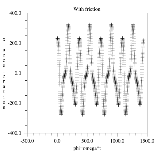
Figure 20: Acceleration in the $x$ direction of the center–of–mass of the rod as a function of time (low friction).

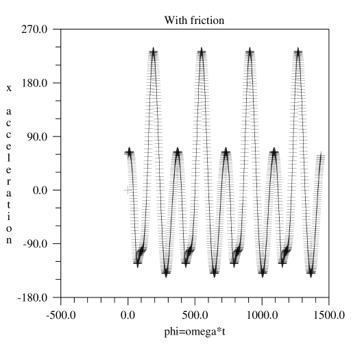
Figure 21: Acceleration in the $x$ direction of the center–of–mass of the rod as a function of time (high friction).

Similar results hold for the acceleration in the $y$–direction. These graphs were generated with a particular set of parameters and initial conditions of the model whose precise values are not important for our purposes here. The interesting aspect is that the acceleration in, say, the $x$ direction shows a definite bias in favor of being larger in magnitude in for, in this case, positive values over negative values.

Let us imagine that we place this mechanical model on a cart which is resting on a surface and let it begin its motion. The acceleration of the rod will, by Newton’s 3^rd law, cause a back reaction, causing the cart to oscillate back and forth. First assume the surface is frictionless. Even though the acceleration of the rod is larger in one particular direction than the opposite one, the cart will not show any net movement – the larger acceleration in, say, the $+x$ direction is compensated by the smaller acceleration in the $-x$ directions which lasts for comparatively longer periods of time. However, let us now imagine that there is some friction between the cart and the surface. It is possible, with the right combination of parameters and initial conditions, that this friction “absorbs” the back reaction in the direction for which the acceleration is smallest, but doesn’t completely absorb the back reaction in the other direction. In this case the cart can “push off” the surface, and exhibit a net motion.

Similar effects will hold for motion in the $y$ direction, and so the net motion will be a combination of motion in both directions. However, if we place two such mechanical devices on the cart and have them rotate in opposite directions, the back reactions in, say, the $y$ direction can be arranged to cancel, leaving a net motion in only the $x$ direction. Such a device has been constructed (U. S. Patent #4,631,971 and U. S. Patent Application #268,914); one rather striking illustration of its operation is that the device, self–contained within a box, when placed in a canoe in a swimming pool, will propel the canoe in one particular direction, without the need for a propeller in contact with the water.

Although perhaps surprising, the principle behind this device is intuitively known to many children. Have a child sit on a piece of cardboard on a smooth floor and then tell her to move forward by rocking. If one watches closely, the child will rock in one direction quickly and return in the other direction slowly. The change in momentum of the child leads to a reactive force being transferred to the cardboard, but the uneven rocking results in this force overcoming the frictional force in only one particular direction. The net result is that the child will propel herself in one direction.

X Conclusions

In this paper we have studied a simple mechanical model of a periodically driven nonlinear mechanical system. Bifurcation diagrams, dimensions, power spectra, and Lyapunov exponents were derived in order to locate regions of quasiperiodic, periodic and chaotic behavior within the parameter space of the system. Within the parameter space is the the coexistence of a chaotic attractor and a limit cycle, which implies that initial conditions may determine whether the system will exhibit periodic or chaotic behavior. We also discussed some aspects of the model as it relates to a propulsion device. This system, although relatively simple, exhibits a rich behavior with a number of interesting non–linear effects being present.

We have also performed a symbolic analysis of the model. By constructing the proper Poincaré section in the phase space for a system of ODEs, the symbolic dynamics can be constructed based on the appropriate partitioning of the phase portrait and it turns out to be an efficient and powerful way to explore the global properties of the system both in the phase and parameter spaces. Up to now, the symbolic dynamics has been applied to the analysis of the NMR–laser chaos model zl95 ; lwz96 , the two–well Duffing equation xzh95 , the forced Brusselator lz95 ; lzh96 , and the Lorenz model fh96 ; zl97 ; hlz98 , in addition to the system discussed in this paper. Along a certain direction in the parameter space this model exhibits various properties, such as, periodicity, quasiperiodicity, chaos, 1D and 2D features, etc. In some other directions or regions of the parameter space the model would also display more or less similar behavior. We have established the 3-letter symbolic dynamics for the model and found that the ordering rules of sequences, the forced Brusselator in the regime of annular dynamics and the dissipative standard map at some parameters are the same. As a matter of fact, the NMR-laser chaos model, the forced Brusselator in the regime of interval dynamics and the Hénon map with a positive Jacobian also have similar 2-letter symbolic dynamics and share the same ordering rules of sequences. It, therefore is meaningful in a sense to classify the systems of ODEs according to their ordering rules of sequences. The ODEs investigated under the guidance of symbolic dynamics to day are quite limited though.

References

- (1) N. Metropolis, M. L. Stein, and P. R. Stein, J. Combinat. Theory A15, 25 (1973).
- (2) Hao Bai-lin, Elementary Symbolic Dynamics and Chaos in Dissipative Systems, (World Scientific, Singapore, 1989).
- (3) M. Hénon, Commun. Math. Phys. 50, 69 (1976).
- (4) R. Lozi, J. de Physique 39C, 9 (1978).
- (5) W.-M. Zheng, and J.-X. Liu, Phys. Rev. E50, 3241 (1994).
- (6) P. Grassberger, and H. Kantz, Phys. Lett. 113A, 235 (1985).
- (7) P. Cvitanović, G. H. Gunaratne, and I. Procaccia, Phys. Rev. A38, 1503 (1988).
- (8) Y. Gu, Phys. Lett. A124, 340 (1987).
- (9) J.-X. Liu, and W.-M. Zheng, Commun. Theor. Phys. 23, 315 (1995).
- (10) J.-X. Liu, W.-M. Zheng, and B.-L. Hao, Chaos, Solitons and Fractals 7, 1427 (1996).
- (11) F.-G. Xie, W.-M. Zheng, and B.-L. Hao, Commun. Theor. Phys. 24, 43 (1995).
- (12) W.-M. Zheng, and J.-X. Liu, Phys. Rev. E51, 3735 (1995).
- (13) J.-X. Liu, Z.-B. Wu, and W.-M. Zheng, Commun. Theor. Phys. 25, 149 (1996).
- (14) H.-P. Fang, Z. Phys. B96, 547 (1995).
- (15) H.-P. Fang, and B.-L. Hao, Chaos, Solitons and Fractals 7, 217 (1996).
- (16) W.-M. Zheng, and J.-X. Liu, Commun. Theor. Phys. 27, 423 (1997).
- (17) B.-L. Hao, J.-X. Liu, and W.-M. Zheng, Phys. Rev. E57, 5378 (1998).
- (18) B.-L. Hao, Chao-dyn/9806025.
- (19) W.-M. Zheng, Int. J. Mod. Phys. 5B, 481 (1991); Chaos, Solitons and Fractals 4, 1221 (1994).
- (20) R. Ito, Math. Proc. Camb. Phil. Soc. 89, 107 (1981).
- (21) V. I. Oseledec, Trans. Mosc. Math. Soc. 19, 197 (1968).
- (22) G. Benettin, L. Galgani, A. Giorgilli and J. Strelcyn, Meccanica, Vol. 15, No. 1, 9-19 (1980).
- (23) I. Shimada and T. Nagashima, Prog. The. Physics, Vol. 61, No. 6, 1605-16 (1979).
- (24) A. Wolf, J. B. Swift, H. L. Swinney and J. A. Vastano, Physica 16D 285-317 (1984).
- (25) H. Haken, Physics Letters 94A, No. 2, 71-72 (1983).
- (26) S. Peleš, Prog. The. Physics Suppl. No. 139, p. 496-506 (2000).
- (27) K. T. Alligood, T. D. Sauer, J. A. Yorke, Chaos, an Introduction to Dynamical Systems, p. 238. Springer-Verlag New York, Inc. (1997).
- (28) P. Grassberger and I. Procaccia, Physica 13D, 34-54 (1984).
- (29) J. L. Kaplan and J. A. Yorke, Lecture Notes in Mathematics, Vol. 730, 204-227, Springer-Verlag, Berlin (1979).
- (30) F. Ledrappier, Commun. Math. Phys. 81, 229-238 (1981).
- (31) J. D. Farmer, E. Ott and J. A. Yorke, Physica 7D, 153-180 (1983).
- (32) P. Manneville and Y. Pomeau, Physics Letters 75A, No. 1,2, 1-2 (1979).
- (33) C. Grebogi, E. Ott and J. A. Yorke, Physica 7D, 181-200 (1983).
- (34) S. W. McDonald, C. Grebogi, E. Ott and J. A. Yorke, Physica 17D, 125-153 (1985).
- (35) H. Nusse and J. A. Yorke, Dynamics: Numerical Exploration, Springer-Verlag New York, Inc. p. 317 (1998).