Ghost orbit bifurcations in semiclassical spectra

Abstract

Gutzwiller’s semiclassical trace formula for the density of states in a chaotic system diverges near bifurcations of periodic orbits, where it must be replaced with uniform approximations. It is well known that, when applying these approximations, complex predecessors of orbits created in the bifurcation (“ghost orbits”) can produce clear signatures in the semiclassical spectra. We demonstrate that these orbits themselves can undergo bifurcations, resulting in complex, non-generic bifurcation scenarios. We do so by studying an example taken from the Diamagnetic Kepler Problem. By application of normal form theory, we construct an analytic description of the complete bifurcation scenario, which is then used to calculate the pertinent uniform approximation. The ghost orbit bifurcation turns out to produce signatures in the semiclassical spectrum in much the same way as a bifurcation of real orbits would.

1 Introduction

Since its discovery in the early 1970s, Gutzwiller’s trace formula [1] has become a widely used tool for the interpretation of quantum spectra of systems whose classical counterpart exhibits chaotic behaviour. It represents the density of states of the quantum system as a sum over a smooth part and fluctuations from all periodic orbits of the classical system, which are all calculated from purely classical data. This formula assumes all periodic orbits to be isolated, so that it fails close to a bifurcation of periodic orbits, where different orbits approach one another arbitrarily closely, leading to a divergence of the periodic orbit contributions.

This failure can be overcome with the help of uniform approximations [2, 3, 4, 5] which take into account the contributions of all bifurcating orbits collectively. Although in generic Hamiltonian systems only codimension-one bifurcations can be observed as a single control parameter is varied, in practical applications of uniform approximations bifurcation scenarios of higher codimensions must be included:[6, 7]  If a periodic orbit successively undergoes several bifurcations, uniform approximations capable of collectively treating all orbits participating in the whole complicated bifurcation scenario are needed.

In the construction of most uniform approximations known, ghost orbits [8] in the complexified classical phase space play a crucial role, because real periodic orbits that are born in a bifurcation tend to have ghost orbit predecessors before they turn real. So far, these ghost orbits have never been observed to undergo bifurcations themselves, although there is no a priori reason why this should be impossible. In fact, we will now present an example of a ghost orbit bifurcation which occurs in connection with a generic period-quadrupling bifurcation of a real orbit. We will show that the construction of a uniform approximation requires the inclusion of this bifurcation and that traditional normal form theory can be extended to also cover bifurcations of ghost orbits. A more detailed presentation of our results can be found in Bar1,Bar2.

2 The bifurcation scenario

As an example, we study the hydrogen atom in a magnetic field, which has been described in detail, e.g., in Refs. Fri89,Has89,Wat93. We assume the nucleus fixed and regard the electron as a structureless point charge. Due to a scaling property of the Hamiltonian, the classical dynamics does not depend on the energy $E$ and the magnetic field strength $\gamma$ separately, but only on the scaled energy $\tilde{E}=\gamma^{-2/3}E$. To plot periodic orbits, we use scaled semiparabolical coordinates $\mu^{2}=\tilde{r}+\tilde{z},\ \nu^{2}=\tilde{r}-\tilde{z}$.

To look for ghost orbits, we complexify the classical phase space by allowing coordinates and momenta to assume complex values. Since our Hamiltonian is real, the system is symmetric with respect to complex conjugation. Therefore, the complex conjugate of a periodic orbit is a periodic orbit itself, so that orbits usually occur in complex conjugate pairs. In exceptional cases, however, a periodic ghost orbit can coincide with its complex conjugate. These symmetric ghost orbits then have real periods and actions.

Figure 1: Real orbits at scaled energy $\tilde{E}=-0.340>\tilde{E}_{c}$, drawn in scaled semiparabolical coordinates. Solid and dashed curves: stable and unstable satellite orbits. Dotted curve: balloon orbit

One of the shortest periodic orbits of the diamagnetic Kepler problem is the balloon orbit, which we will now focus attention on. It undergoes a period-quadrupling at a scaled energy of (in scaled atomic units, which we use throughout) $\tilde{E}_{c}=-0.342\,025$. If $\tilde{E}>\tilde{E}_{c}$, a stable and an unstable real satellite orbit of quadruple period exist. At $\tilde{E}_{c}$, they simultaneously collide with the balloon orbit and vanish. The real orbits are shown in figure 1 at the scaled energy of $\tilde{E}=-0.340$. The solid and dashed curves represent the stable and unstable satellite orbits, respectively. For comparison, the balloon orbit is shown as a dotted curve. If $\tilde{E}<\tilde{E}_{c}$, no real satellites are present, but there are a stable and an unstable ghost orbit instead, both of which are symmetric with respect to complex conjugation. Thus, at $\tilde{E}_{c}$ a generic island-chain bifurcation takes place.

Figure 2: Real and imaginary parts of complex ghost orbits at scaled energy $\tilde{E}=-0.343$. Solid and dotted curves: stable and unstable ghost satellites created in the period-quadrupling bifurcation of the balloon orbit at $\tilde{E}_{c}=-0.342\,025$. Dashed curve: additional ghost orbit created in the ghost bifurcation at $\tilde{E}_{c}^{\prime}=-0.343\,605$.

Figure 3: Ghost orbits at scaled energy $\tilde{E}=-0.344<\tilde{E}_{c}^{\prime}$. Solid and dashed curves: asymmeric ghost orbits (real parts coincide) created at the ghost bifurcation at $\tilde{E}_{c}^{\prime}=-0.343\,605$. Dotted curve: unstable ghost satellite created at the period-quadrupling bifurcation of the balloon orbit

Furthermore, there is an additional ghost orbit in the phase space close to this bifurcation that is also symmetric with respect to complex conjugation. At $\tilde{E}_{c}^{\prime}=-0.343\,605<\tilde{E}_{c}$, this orbit collides with the stable ghost satellite, the two orbits loose their symmetry and become a pair of complex conjugate ghosts at $\tilde{E}<\tilde{E}_{c}^{\prime}$. For scaled energies above and below $\tilde{E}_{c}^{\prime}$, the ghost orbits are depicted in figures 3 and 3, respectively. From the imaginary parts it can clearly be seen that the symmetry with respect to complex conjugation is lost in the bifurcation.

This is the first example of a ghost orbit bifurcation that has been described in the literature. Its occurrence presents an additional challenge to the construction of a uniform approximation because an approximation that deals with the generic period quadrupling bifurcation only diverges at the bifurcation energy of the ghost orbit bifurcation and becomes undefined below $\tilde{E}_{c}^{\prime}$ where the stable ghost satellite orbit used in its construction does not exist any more.

All periodic orbit parameters required for the construction of the uniform approximation were calculated numerically. The complete numerical data is described in detail in Bar1,Bar2. As an example, the orbital periods are shown in figure 4. From the successive confluences of the periods, the sequence of bifurcations becomes clearly visible: The period of four repetitions of the balloon orbit, which is always real, is indicated by a nearly horizontal line at $\tilde{T}\approx 5.84$. Above $\tilde{E}_{c}$, there are two additional solid curves representing the periods of the stable (upper curve) and unstable (lower curve) real satellite orbits. At $\tilde{E}_{c}$, these curves change from solid to dashed as the satellite orbits become ghosts. Below $\tilde{E}_{c}$, the unstable ghost satellite does not undergo any further bifurcations in the energy range shown, whereas the stable satellite collides, at $\tilde{E}_{c}^{\prime}$, with the additional ghost orbit. The latter can clearly be seen not to be involved in the bifurcation at $\tilde{E}_{c}$. Below $\tilde{E}_{c}^{\prime}$, these two orbits are complex conjugates of each other. Thus, the real parts of their periods coincide, whereas the imaginary parts are different from zero and have opposite signs.

Figure 4: Orbital periods of the orbits involved in the bifurcations as functions of the scaled energy $\tilde{E}=E\gamma^{-2/3}$

3 The general form of the uniform approximation

Before we return to classical normal form theory in section 4, we introduce, in this section, the basic formulas for the quantum density of states necessary for the construction of the uniform semiclassical approximation. The density of states of a quantum system with the Hamiltonian $\hat{H}$ can be expressed with the help of the Green’s function $G(E)=(E-\hat{H})^{-1}$ as

$$d(E)=-\frac{1}{\pi}\,{\rm Im}\,{\rm Tr}\,\,G(E)\;,$$ (1)

where the trace of the Green’s function can be evaluated in the coordinate representation,

$${\rm Tr}\,\,G(E)=\int d\mib{x^{\prime}}d\mib{x}\,\delta(\mib{x^{\prime}}-\mib{x})\,G(\mib{x^{\prime}}\mib{x},E)\;.$$ (2)

The first step in the formulation of periodic orbit theory [1] is to replace the Green’s function $G(\mib{x^{\prime}}\mib{x},E)$ with its semiclassical Van Vleck-Gutzwiller approximation. For systems with two degrees of freedom the semiclassical approximation to the Green’s function reads

$$G(\mib{x^{\prime}}\mib{x},E)=\frac{1}{i\hbar\sqrt{2\pi i\hbar}}\sum_{\rm class.~{}traj.}\sqrt{D}\exp\left\{\frac{i}{\hbar}S(\mib{x^{\prime}}\mib{x},E)-i\frac{\pi}{2}\nu\right\}\;.$$ (3)

Here, the sum extends over all classical trajectories running from $\mib{x}$ to $\mib{x^{\prime}}$ at energy $E$, $S$ is the action of a trajectory, $\nu$ its Maslov index, and $D$ is given in terms of second derivatives of the action. The contribution of a single orbit to the trace can be evaluated by introducing coordinates parallel and perpendicular to the orbit. The integration along the orbit can then be performed in a straightforward fashion. If one notes that on a periodic orbit the action $S(\mib{x^{\prime}}\mib{x},E)$ is stationary with respect to the transverse coordinates, Gutzwiller’s trace formula for isolated periodic orbits is finally obtained by integrating over the transverse coordinates using the stationary-phase approximation. It is this last step which fails close to a bifurcation, where periodic orbits are not isolated.

The basic idea of the stationary-phase approximation is to approximate the action function by a quadratic function in the neighbourhood of any individual periodic orbit. To achieve a collective treatment of the bifurcating orbits, we need to find an ansatz function $\Phi$ on a Poincaré surface of section which has got stationary points corresponding to all periodic orbits to be included in the uniform approximation. We can then relate $\Phi$ to the classical action function $S(\mib{x^{\prime}}\mib{x},E)$ by means of a suitable, albeit unknown, coordinate transformation. In terms of $\Phi$, the uniform approximation can be shown to assume the form [3]

$$d(E)=\frac{1}{2\pi^{2}m\hbar^{2}}\,{\rm Re}\,\exp\left\{\frac{i}{\hbar}S_{0}(E)-i\frac{\pi}{2}\hat{\nu}\right\}\int dY\,dP_{Y}^{\prime}\,X(Y,P_{Y}^{\prime})\,\exp\left\{\frac{i}{\hbar}\Phi(Y,P_{Y}^{\prime})\right\}\;.$$ (4)

The coefficient $X$ can be evaluated at the stationary points of $\Phi$, where it assumes the value

$$X\stackrel{{\scriptstyle\rm sp}}{{=}}\frac{\{m\}T}{\sqrt{|{\rm Tr}\,M-2|}}\sqrt{|{\rm Hess}\,\Phi|}\;.$$ (5)

Here, $T$ and $M$ denote the period and the monodromy matrix of the corresponding classical orbit, ${\rm Hess}\,\Phi$ the Hessian determinant of the normal form, and the notation $\{m\}$ is meant to indicate that this factor does not occur at the satellite orbits.

4 Normal-form description of the bifurcation

A systematic means to construct an ansatz function $\Phi$ is provided by normal form theory.[14, 15]  Here, we adopt a normal form used by Schomerus [16] to describe codimension-two bifurcations. In canonical polar coordinates $(I,\varphi)$, which are connected to Cartesian coordinates $(p,q)$ by

$$p=\sqrt{2I}\,\cos\varphi\;,\qquad q=\sqrt{2I}\,\sin\varphi\;,$$ (6)

it reads

$$\Phi=\varepsilon I+aI^{2}+bI^{2}\cos(4\varphi)+cI^{3}(1+\cos(4\varphi))\;.$$ (7)

This normal form turns out to qualitatively describe the sequence of bifurcations encountered here for suitably chosen parameter values.

To establish the connection to the classical bifurcation scenario, we have to determine the stationary points of $\Phi$. The central periodic orbit at $I=0$ does not show up as a stationary point because the polar coordiante system (6) is singular there. In the case $|a|>|b|$ and $c<0$ we find three stationary points, each of which appears at four different angles $\varphi$ because it corresponds to an orbit of quadruple period. For these stationary points, the real parts of the action coordinates $I$ are shown in figure 5. The dotted line in this figure corresponds to a pair of complex conjugate stationary points.

To interprete these results, we observe that according to its definition (6) the coordinate $I$ is positive for real orbits and that the action $\Phi(I,\varphi)$ is real for real $I,\varphi$. Therefore, negative real solutions $I$ correspond to ghost orbits which are symmetric with respect to complex conjugation and thus have real actions, whereas a complex $I$ indicates an asymmetric ghost orbit.

Figure 5: A sketch of the bifurcation scenario given by the normal form (7) for the case $|a|>|b|$ and $c<0$. Solid curves: real orbits. Dashed curves: ghost orbits symmetric with respect to complex conjugation. Dotted curve: a pair of complex conjugate ghosts.

If $\varepsilon>0$, we have two stationary points at positive values of $I$ and one stationary point at a negative $I$. They correspond to two real satellite orbits of quadruple period and a symmetric ghost orbit. As $\varepsilon$ decreases through zero, two stationary points simultaneously move from positive to negative $I$, thus indicating that the two real satellites become ghosts in an island-chain bifurcation. Finally, two stationary points with negative action coordinates collide at a negative value of $\varepsilon$ and become complex. This describes a ghost orbit bifurcation in which two symmetric ghost orbits collide and loose their symmetry.

The normal form (7) thus qualitatively reproduces the bifurcation scenario described above. The normal form parameters $\varepsilon,a,b,c$ have to be determined so as to make the description quantitatively correct. To this end we calculate the stationary values of the normal form, equate them to the actions of the periodic orbits and then solve for the normal form parameters. As can be shown by a lengthy calculation,[10]  these parameters are uniquely determined by the actions and the energy if we choose $\varepsilon=\tilde{E}-\tilde{E}_{c}$ and require all parameters to depend continuously on the energy.

5 Evaluation of the uniform approximation

After the ansatz function $\Phi$ has been completely specified, a suitable approximation to the coefficient $X$ in (4) remains to be found. We assume $X$ to be independent of $\varphi$, and as the value of $X$ is known at the stationary points of $\Phi$ at four different values of $I$ (including $I=0$), we approximate $X$ by the third order polynomial $p(I)$ interpolating between the four given points. This choice ensures that our approximation reproduces Gutzwiller’s isolated-orbits formula if, sufficiently far away from the bifurcations, we evaluate the integral in stationary-phase-approximation. Thus, the uniform approximation takes its final form

$$d(E)=\frac{1}{2\pi^{2}m\hbar^{2}}\,{\rm Re}\,\exp\left\{\frac{i}{\hbar}S_{0}(E)-i\frac{\pi}{2}\hat{\nu}\right\}\int dY\,dP_{Y}^{\prime}\,p(I)\,\exp\left\{\frac{i}{\hbar}\Phi(Y,P_{Y}^{\prime})\right\}\;,$$ (8)

which contains known functions only and can be evaluated numerically.

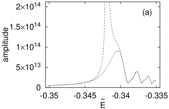
Figure 6: Uniform approximation to the contribution of the considered bifurcations to the density of states for two different values of the magnetic field strength: $(a)\gamma=10^{-12}$, $(b)\gamma=10^{-14}$. Solid curves: uniform approximations. Dashed curves: Gutzwiller’s trace formula.

We calculated the uniform approximation (8) for two different values of the magnetic field strength $\gamma$. The results are shown in figure 6. To suppress the highly oscillatory contributions originating from the factor $\exp\left\{\frac{i}{\hbar}S_{0}(E)\right\}$, we plot the absolute value of (8) instead of the real part. As can be seen, the uniform approximation proposed is finite at the bifurcation energies, and, as the distance from the bifurcations increases, asymptotically goes over into the results of Gutzwiller’s trace formula. Even the complicated oscillatory structures in the density of states caused by interferences between the contributions from the different real orbits involved at $\tilde{E}>\tilde{E}_{c}=-0.342\,025$ are perfectly reproduced by our uniform approximation. We also see that the higher the magnetic field strength, the farther away from the bifurcation the asymptotic (Gutzwiller) behaviour is acquired. The magnetic field dependence of the transition into the asymptotic regime can be traced back to the fact that, due to the scaling properties of our system, the scaling parameter $\gamma^{1/3}$ plays the rôle of an effective Planck’s constant, therefore the lower $\gamma$ becomes, the more accurate the semiclassical approximation will be.

6 Conclusion

We have shown that in Hamiltonian systems with mixed regular-chaotic dynamics ghost orbit bifurcations can occur besides the bifurcations of real orbits. These are of special importance when they appear in the vicinity of bifurcations of real orbits, since they turn out to produce signatures in the semiclassical spectra much the same as those of the real orbits. Consequently, the traditional theory of uniform approximations for bifurcations of real orbits must be extended to also include the effects of bifurcating ghost orbits.

We have illustrated the phenomenon of bifurcating ghost orbits in the neighbourhood of bifurcations of real orbits by way of example for the period-quadrupling of the balloon orbit in the diamagnetic Kepler problem, and have demonstrated how normal form theory can be extended for this case so as to allow for a unified description of both real and complex bifurcations.

We picked the example mainly for its simplicity, since (a) the real orbit considered is one of the shortest fundamental periodic orbits in the diamagnetic Kepler problem and (b) the period-quadrupling is the lowest period-$m$-tupling possible ($m=4$) that exhibits the island-chain bifurcation typical of all higher $m$. Thus we expect ghost orbit bifurcations to appear also for longer-period orbits, and, in particular, in the vicinity of all higher period-$m$-tupling bifurcations of real orbits.

In fact, a general discussion[10] of the bifurcation scenarios described by the normal form (7) and a more general variant of its for different values of the parameters leads us to the conclusion that the appearance of ghost orbit bifurcations in the vicinity of bifurcating real orbits is the rule, rather than the exception, in general systems with mixed regular-chaotic systems, and thus one of their generic features.

References

- [1] M. C. Gutzwiller, \JMP8,1967,1979; \andvol12,1971,343.
- [2] A. M. Ozorio de Almeida and J. H. Hannay, \JPA20,1987,5873.
- [3] M. Sieber, \JPA29,1996,4715.
- [4] H. Schomerus and M. Sieber, \JPA30,1997,4537.
- [5] M. Sieber and H. Schomerus, \JPA31,1998,165.
- [6] J. Main and G. Wunner, \PRA55,1997,1743.
- [7] H. Schomerus, \JLEurophys. Lett.,38,1997,423.
- [8] M. Kuś, F. Haake, and D. Delande, \PRL71,1993,2167.
- [9] T. Bartsch, J. Main, and G. Wunner, \JPA32,1999,3013.
- [10] T. Bartsch, J. Main, and G. Wunner, \ANN277,1999,19
- [11] H. Friedrich and D. Wintgen \JLPhys. Rep.,183,1989,37.
- [12] H. Hasegawa, M. Robnik, and G. Wunner, \JLProg. Theor. Phys. Suppl.,98,1989,198.
- [13] S. Watanabe, in Review of Fundamental Processes and Applications of Atoms and Ions, ed. C. D. Lin (World Scientific, Singapore, 1993).
- [14] G. D. Birkhoff, Dynamical Systems (AMS Colloquium Publications vol. IX, Providence, RI, 1927,1966).
- [15] F. Gustavson, \JLAstron. J.,71,1966,670.
- [16] H. Schomerus, \JPA31,1998,4167.