Quasiperiodic patterns in boundary-modulated excitable waves

Abstract

We investigate the impact of the domain shape on wave propagation in excitable media. Channelled domains with sinusoidal boundaries are considered. Trains of fronts generated periodically at an extreme of the channel are found to adopt a quasiperiodic spatial configuration stroboscopically frozen in time. The phenomenon is studied in a model for the photo-sensitive Belousov-Zabotinsky reaction, but we give a theoretical derivation of the spatial return maps prescribing the height and position of the successive fronts that is valid for arbitrary excitable reaction-diffusion systems.

PACS numbers: 05.45.+b, 47.20.Ky, 03.40.Kf, 84.30.Bv

Excitable media display a very rich spatio-temporal behavior with regimes ranging from fairly well ordered structures of propagating waves [1] to highly uncorrelated spatio-temporal chaos. The study of all these features as well as their mutual connections provides very useful insight to understand and eventually control phenomena of paramount applied importance such as the deadly arisal of fibrillation in cardiac tissues[2] or the appearance of either ordered or turbulent patterns in extended chemical reactors operating away from equilibrium conditions. In many of these applications, a crucial but frequently ignored ingredient is the presence of boundaries. For example, it has been shown that boundaries and obstacles in inhomogeneous media are important to either pin or repele spiral patterns [3]; moving boundaries [4] and stripped configurations [5, 6] have also strong effects.

Unfortunately, the current understanding of boundary effects in nonlinear partial differential equations is rather incomplete, and sometimes surprisingly nontrivial behavior lurk behind the apparent simplicity of some problems. A recent study[7], for example, shows that relatively regular boundary conditions such as Dirichlet’s on the banks of a sausage-shaped channel can elicit several types of spatial complexity such as frozen quasiperiodicity and chaos even in very simple reaction diffusion equations. There, the axial coordinate along the channel acts as a “time” in the equations describing the time-independent spatial patterns and the undulated boundaries play the role of a periodic force inducing chaos in a dynamical system that is non-chaotic in the absence of driving.

On the other hand, propagation of waves in excitable media has been studied in a variety of contexts[1]. Due to their ubiquity in large two-dimensional systems, much of this work deals with spiral waves and focuses, in particular, on the various aspects of the behavior around the cores of the spiral patterns. In contrast, the propagation of front trains has received much less attention. This may seem surprising since the same spirals can be seen far from their cores as a periodic train of two-dimensional traveling fronts. These trains, though, are easily characterized by a dispersion relation $c=c(\lambda)$, giving a relation between the constant front train velocity and its uniform spacing $\lambda$ and their dynamics is very simple. However, much less trivial behavior appears even in one-dimensional systems if the excitable medium recovers the rest state not monotonically but via damped oscillations[8]. In this regime, propagating wave trains often relax to irregularly spaced configurations of fronts that can be seen as spatial chaos.

The purpose of this Letter is to report a new kind of nontrivial spatial structure arising as a pure boundary effect in excitable media, namely, stroboscopically-frozen quasiperiodicity. We investigate the asymptotic propagation of excitable wave trains generated by local time-periodic stimulation at the extreme of a sinusoidally undulated channel. We find that contrarily to intuitive expectations, the trains of fronts asymptotically accommodate in quasiperiodic spatial configurations, incommensurated with the boundaries but periodic in time and synchronized with the stimuli. With the experiments on the photosensitive Belousov-Zhabotinsky reaction in mind [4, 6], we demonstrate this phenomenon in the Oregonator model adapted to include the effect of light. Finally, we present a more general semi-analytic theory of the formation of the quasi-periodic, and possibly chaotic, structures referred above.

Photosensitive $Ru(bby)_{3}^{+2}$-catalyzed Belousov-Zhabotinsky reactive media can be modelled [9] by the following version of the Oregonator model:

$$\frac{\partial\,u}{\partial\,t} = \frac{1}{\varepsilon}\left(u\,-\,u^{2}\,-\,(f\,v\,+\,\phi)\,\frac{u\,-\,q}{u\,+\,q}\right)\,+\,D_{u}\,\nabla^{2}u$$ (1)

$$\frac{\partial\,v}{\partial\,t} = (u\,-\,v)\ .$$ (2)

Here $u$ (resp. $v$) describe $HBrO_{2}$ (resp. catalyst) concentrations. $D_{u}$ is a diffusion coefficient and $f$, $q$ , $\varepsilon$ and $\phi$ are parameters related to the reaction kinetics. In our simulations we set $f=3$, $q=0.002$, $\varepsilon=0.05$, $\phi=0.002$ and $D_{u}=1$.

We simulate this reaction in a spatial domain tailored as an undulated channel along the longitudinal direction $x$. The transversal coordinate $y$ is bounded by two sinusoidal walls of common spatial frequency $k=2\pi/\lambda_{p}$, amplitude $d$, minimum separation $s$, and phase mismatch $\eta$:

$$y_{0}(x) = \frac{d}{2}[1-\cos(kx)]$$ (3)

$$y_{1}(x) = -s-\frac{d}{2}[1+\cos(kx+\eta)]$$ (4)

We will concentrate on symmetric sausage-shaped channels ($\eta=\pi$) of width $w(x)=s+d-d\cos(kx)$, as the one shown in Fig. 1. On the sinusoidal boundaries we impose the Dirichlet condition $u=0.004$, a value close to the fixed point of the local dynamics.

In order to solve numerically Eq. (2) it is convenient to map the region limited by $y_{0}(x)$ and $y_{1}(x)$ and by $x=0,L$ to a rectangle: $\widetilde{y}_{1}=1$, $\widetilde{y}_{0}=0$, and $x=0,L$, where $\widetilde{y}=(y-y_{0})/(y_{1}-y_{0})$ and $L$ is the length of the channel. Under this map, the diffusion term transforms as[7]:

$$\nabla^{2}u\rightarrow\partial^{2}_{xx}\widetilde{u}+F(x)\partial^{2}_{\widetilde{y}\widetilde{y}}\widetilde{u}+G(x)\partial^{2}_{x\widetilde{y}}\widetilde{u}+H(x)\partial_{\widetilde{y}}\widetilde{u}\ ,$$ (5)

$F(x)$, $G(x)$ and $H(x)$, given in [7], are periodic functions reflecting the undulations of the boundaries via modulations measured by the product $kd$. In the limit $kd\rightarrow 0$ (straight channel), Eq.(5) becomes the standard Laplacian.

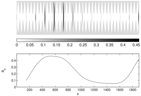
FIG. 1.: In the upper panel, the white area limited by gray undulated boundaries is the excitable region where fronts originated at the left end propagate. The transverse features are the fronts travelling to the right. Darker fronts have a larger value of $u$, as indicated in the colorbar. The lower panel displays the envelope of the maximum amplitude of the fronts.

Wave trains are generated stimulating the medium at the left end $x=0$ of the channel by pushing $u$ above and below the excitability threshold periodically in time. The opposite end of the channel is set as a no-flux boundary. During the simulations we mainly varied the forcing parameters $\lambda_{p}$ and $d$, but also several wave train periods and channel widths were investigated. After a transient, the fields $u$ and $v$ converge to a configuration of propagating fronts that repeats itself periodically in time in synchrony with the wave generator at $x=0$. In other words, the train becomes a stroboscopically frozen pattern. We denote by $x_{n}$ and $a_{n}$ the longitudinal position and maximum height of $u$ at the channel axis, respectively, for the $n$-th front.

As a comparison, in a straight channel ($d=0$) of finite width $s$ the asymptotic configuration of the wave fronts is equally spaced by a length $\lambda$ and propagates with velocity $c=\lambda/T$ if the forcing period is $T$. This velocity increases with the channel width [6] starting from a critical value $s_{c}$ of the latter, below which the fronts cannot propagate. In Fig. 2 we plot the train velocity and the maximum amplitude of the wave fronts as a function of the width of the straight channel.

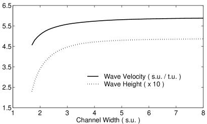
FIG. 2.: Wave train velocity and wave height (multiplied by a factor 10) in straight channels of different widths. There is a critical value, $s_{c}=1.65$, below which propagation becomes impossible. $T=5$.

In modulated domains with $d\neq 0$ a wide range of new spatial configurations incommensurated with the boundaries emerge. Typically, both the spacing and the amplitude of the fronts become spatially quasiperiodic. According to the strength $kd\propto d/\lambda_{p}$, of the spatial forcing we distinguish strong from weak modulations. Let us describe the cases $\lambda_{p}=50$ and $\lambda_{p}=1000$, respectively, as an illustration.

The results for strong modulation are shown in Fig. 3. The amplitude of the boundary undulation increases from top to bottom. The quasiperiodic behavior of the pulse height becomes evident as $d$ increases. The second column in Fig. 3 shows also the maximum $a_{n}$ of each front as a function of its position modulo $\lambda_{p}$. This plot provides information about the distribution of the front height maxima relative to the elementary unit of the channel. Notice that the fronts do not always reach their minimal height at the narrowest channel sections ($x=m\lambda_{p}$) as one would naively expect from the behavior in straight channels depicted in Fig. 2. Moreover, the fronts can now propagate even when the channel is narrower ($s=1.1$) in some places than the minimun width $s_{c}=1.65$ that allows propagation in straight channels. Last column in Fig. 3 displays the return maps of the $(n+1)$-th front position $x_{n+1}$ (relative to the unit channel cell) as a function of the position $x_{n}$ of the previous front. The shapes of the curves are analog to those circle maps describing the temporal dynamics of periodically forced self-oscillators. This analogy suggests that our system should exhibit the same richness of spatial behaviors as the circle map does in time-evolutions.

FIG. 3.: Numerical results obtained from Eq. (2) for strong forcing. First column: Maximum height of each front within the train, as a function of position $x$. Second column: Same as before but with position $x$ folded modulo $\lambda_{p}=50$. Third column: Return map of the front positions modulo $\lambda_{p}$. Each row is for a different amplitude $d$. Parameters: $\lambda_{p}=50$, $T=5$, $s=1.1$. Note that channel length $L=15000$ is much larger that in Fig. 1.

The weak forcing case is illustrated in Fig. 4. As in the case of circle maps for very weak forcing, the front positions return map shows a very small deviation from linearity with the given parameter values. This approximate linearity implies that the front train wavelength is nearly constant and the influence of the channel walls negligible. This influence is, however, more important on the front heights. Minima of front height are situated at the narrowest channel sections, in concordance with Fig. 2, while the maxima saturate for $d$ large enough.

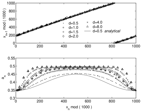
FIG. 4.: Weak forcing behavior at $\lambda_{p}=1000$ and $s=2$. Above: Return map of the front positions modulo $\lambda_{p}$. Below: Maximum height of each front as a function of the front position modulo $\lambda_{p}$. Solid lines are from Eqs. (10) and (12).

Let us now derive a semi-analytical expression for the return maps of successive wave fronts positions and maxima heights. In view of the results for the weak forcing case we assume that the front velocity in the undulated channel at a position where the local width is $w$ adapts quasi-adiabatically to the velocity $c(w)$ (Fig. 2) corresponding to a uniform channel of the same width. Thus, the velocity of the $n$-th front is

$$\dot{x}_{n}(t)=c(w(x_{n}))$$ (6)

In our channel $w(x)=w_{0}-w_{1}\cos(kx)$ with $w_{0}=s+d$ and $w_{1}=d$. In order to proceed analytically an approximation for $c(w)$ should be introduced. For $d$ small the width variation is also small and $c(w)$ can be replaced by a linear fit $a+bw$ of an apropriate range of data in Fig. 2. Hence, $c(w(x_{n}))\approx c_{0}-c_{1}\cos(kx_{n})$ where $c_{0}=a+bw_{0}$ and $c_{1}=bw_{1}$. Eq. (6) can now be integrated during one period $T$ of the front generator, to obtain:

$$\frac{2}{k\sqrt{c_{0}^{2}-c_{1}^{2}}}\left[\arctan f(x_{n})\right]_{x_{n}(0)}^{x_{n+1}(0)}=T$$ (7)

with

$$z_{n}=f(x_{n})=\sqrt{\frac{c_{0}+c_{1}}{c_{0}-c_{1}}}\tan\left(\frac{kx_{n}}{2}\right)$$ (8)

Here we have used the observed time periodicity of the wave train to write $x_{n}(T)=x_{n+1}(0)$, a crucial step to convert the time-differential equation (6) into a map for space positions. Defining $\varphi=\arctan z$ and $\bigtriangleup=0.5\,kT\sqrt{c_{0}^{2}-c_{1}^{2}}$ we have $\bigtriangleup=\varphi_{n+1}-\varphi_{n}$, and the return map for the variable $z$ is

$$z_{n+1}=g(z_{n})=\frac{z_{n}+\tan\bigtriangleup}{1-\tan\bigtriangleup\cdot z_{n}}\ .$$ (9)

In terms of the front position $x$ we finally have:

$$x_{n+1}=f^{-1}\left(g(f(x_{n}))\right)$$ (10)

For the maximum height of the wave fronts, the same adiabaticity assumption leads to $a_{n}=h\left(w_{0}-w_{1}\cos(kx_{n})\right)$, with $h(w)$ being the maximum height of the fronts in a straight channel of width $w$. We can go one step further towards qualitatively describe the observed positional mismatch between the minimal-height fronts and the narrowest channel sections by considering a short adaptation time $\tau_{a}$ of the front characteristics to the local width:

$$\dot{a}_{n}(t)=\frac{1}{\tau_{a}}\left(h(w(x_{n}))-a_{n}\right)$$ (11)

As above, by linearly fitting the data from Fig. 2 in the range $(s,s+2d)$ we have $h(w)\approx a^{\prime}+b^{\prime}w$ for small $d$. Then, $h(w(x))\approx h_{0}-h_{1}\cos kx$, with $h_{0}=a^{\prime}+b^{\prime}w_{0}$, and $h_{1}=b^{\prime}w_{1}$. Integrating Eq. (11) for small $d$ and $kc_{0}\tau_{a}\ll 1$ so that we can set $x_{n}(t)=x_{n}(0)+c_{0}t+{\cal O}(d)$, we get a relationship linking the wavefront heights and positions,

$$a_{n+1}=h_{0}-\frac{h_{1}}{\sqrt{1+\tau_{a}^{2}k^{2}v_{0}^{2}}}\sin\left(k(x_{n}+v_{0}T)+\theta\right)\ .$$ (12)

Here $\theta=\arccos(1/\sqrt{1+(\tau_{a}v_{0}k)^{2}})$ describes the displacement of the minimal heights from the narrowest sections.

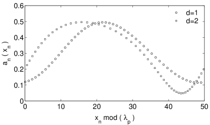
FIG. 5.: Change in the shape of $a_{n}(x_{n})$ from Eq. (12) by increasing $d$ beyond the weak forcing limit. The qualitative trend agrees with Fig. 3.

Since the derivation of Eqs. (10) and (12) is formally valid only in the weak forcing limit we first contrast the theory against the numerical data in Fig. 4 for $d=0.5$, to confirm the good agreement[10]. More detailed numerical explorations reasure us that both adiabaticity and small $d$ approximations are justified and that the small deviations in Fig. 4 are only due to the linear approximation. Moreover, a systematic $d$-expansion in Eq. (10) would lead precisely to a circle map supporting the observation that this model is relevant to the description of our boundary-induced patterns in a given limit. Finally, while the agreement between the theory and the numerics is bound to worsen as forcing increases, the theory still describes well the pattern features in the strong forcing regime. For instance, Fig. 5 shows how the maxima and minima of $a_{n}(x_{n})$ shift as $d$ is increased, in good qualitative agreement with the corresponding case of Fig. 3.

In summary, we have shown that boundary conditions in domains with the form of undulated channels may induce nontrivial longitudinal spatial configurations of propagating trains of excitation fronts generated by a local time-periodic stimulation in simple excitable media. In particular, stroboscopically frozen quasi-periodic arrays of fronts were found. These structures were described in terms of spatial return maps that are very similar to the circle maps whose iteration describe the temporal dynamics of forced oscillators. This similarity allows one to speculate about the existence of even more complex configurations representing the spatial realizations of the chaotic regimes of these maps. The phenomenon reported here should be experimentally observable in the photo-sensitive Belusov-Zhabotinsky reaction with proper lighting conditions at the boundaries. Work along this line is currently in progress.

Finantial support from DGES projects PB94-1167, PB97-0540 and PB97-0141-C01-01 is greatly acknowledged.

REFERENCES

- [1] Chemical Waves and Patterns, edited by R. Kapral and K. Showalter (Kluwer Academic, Dordrecht, 1993).
- [2] A. Garfinkel et al., Proc. Nat. Acad. Sci. 97, 6061 (2000).
- [3] M.Gómez-Gesteira, A.P. Muñuzuri, V. Pérez-Muñuzuri, and V. Pérez-Villar, Phys. Rev. E 53, 5480 (1996); J.M. Davidenko, A.V. Pertsov, R. Salomonsz, W. Baxter, and J. Jalife, Nature 355, 349 (1992); A. Sepulchre and A. Babloyantz, Phys. Rev. E 48, 187 (1993); I. Aranson, D. Kessler and I. Mitkov, Phys. Rev. E 50, R2395 (1994).
- [4] A.P.Muñuzuri, V.A. Davydov, M. Gómez-Gesteira, V. Pérez-Muñuzuri, and V. Pérez-Villar, Phys. Rev. E 54, 1 (1996).
- [5] A.M. Zhabotinsky, M.D. Eager, and I.R. Epstein, Phys. Rev. Lett. 71, 1526 (1993).
- [6] O. Steinbock, V. S. Zykov, and S.C.Müller, Phys. Rev. E 48, 3295 (1993).
- [7] V.M. Eguíluz, E. Hernández-García, O.Piro, and S. Balle, Phys. Rev. E 60, 6571 (1999).
- [8] E. Meron, Phys. Rep. 218, 1 (1992).
- [9] H.J. Krug, L. Pohlmann, and L. Kuhnert, J. Phys. Chem. 94, 4862 (1990).
- [10] Fittings to Fig. 2 lead to , , , and .