Abstract

We derive an exact expression for the two-point correlation function for quantum star graphs in the limit as the number of bonds tends to infinity. This turns out to be identical to the corresponding result for certain Šeba billiards in the semiclassical limit. Reasons for this are discussed. The formula we derive is also shown to be equivalent to a series expansion for the form factor — the Fourier transform of the two-point correlation function — previously calculated using periodic orbit theory.

1 Introduction

The statistical distribution of quantum energy levels is a much studied topic. It has been conjectured that generic, classically integrable systems give rise to uncorrelated quantum spectra [1], while the energy levels of generic classically chaotic systems have the same statistical properties as the eigenvalues of random matrices [2]. This has been confirmed by semiclassical theory [3, 4], and in a large number of numerical studies, but classes of systems have also been found for which it is not true; these include geodesic motion on surfaces of constant negative curvature [5], and the cat maps [6].

Quantum graphs [7, 8] are mathematical models introduced in order to explore the connection between the periodic orbits of a system and the statistical properties of its energy levels. The trace formula, in which the level density is connected to a sum over periodic orbits, is exact for graphs, rather than a semiclassical approximation, and the orbits can be classified straightforwardly. However, despite the fact that numerical computations have revealed good conformance of the spectral statistics of many quantum graphs to the predictions of Random Matrix Theory (RMT), few conclusive analytical results have been obtained so far. This is due to the fact that although some individual finite graphs can be shown to reproduce certain features of RMT behaviour [9, 10, 11], the full RMT results can only be recovered in a limit in which one is forced to consider larger and larger graphs, and this necessitates finding general, combinatorial asymptotic techniques for dealing with the (non-trivial) length degeneracies of the periodic orbits.

One family of graphs in which this goal has been achieved are the star graphs [12] (defined below and shown in Fig. 1), but in this case the resulting spectral statistics are neither RMT nor Poissonian (i.e. those of random numbers). It turns out, however, that it is not the first time that such statistics have arisen in the connection with the study of quantum chaos. Our purpose here is to demonstrate that the star graphs have exactly the same two point spectral correlations as a large class of quantum systems, which we will refer to as Šeba billiards.

The original Šeba billiard, a rectangular quantum billiard perturbed by a point singularity (also illustrated in Fig. 1), was introduced in [13] as an example of a system whose classical counterpart is integrable (the singularity affects only a set of measure zero of the orbits) but which nonetheless exhibits properties of quantum chaos. This construction was later generalized to all integrable systems [14] perturbed in the same way. We will refer to any system in this class as a Šeba billiard.

The energy levels of a Šeba billiard can be found by solving an explicit equation which depends on the levels of the original unperturbed system and on the boundary conditions imposed at the singularity. This equation takes the general form

$$\lambda\xi(z)=1,$$ (1)

where $\xi(z)$ is the meromorphic function

$$\xi(z)=\sum_{n}\frac{|\psi_{n}({\bf x_{0}})|^{2}}{E_{n}-z},$$ (2)

the sum being suitably regularized to ensure convergence. Here $\left\{E_{i}\right\}$ are the eigenvalues of the unperturbed system, $\psi_{n}({\bf x_{0}})$ is the value of the $n$th unperturbed eigenfunction at the position ${\bf x_{0}}$ of the singularity, and the coupling constant $\lambda$ parametrizes the boundary conditions [13, 14]. Assuming that $\left\{E_{i}\right\}$ are given by a Poisson process, one can then calculate the associated spectral statistics, such as the joint level distribution, asymptotics of the level spacing distribution [14], and the two-point spectral correlation function [15]. The results show the presence of spectral correlations but are substantially different from the RMT forms.

Here we apply the methods developed for Šeba billiards in [15] to calculate the two-point spectral correlation function for star graphs, starting from an expression which is analogous to (2). The formula obtained will be shown to be a resummation of the expansion computed from the periodic orbit sum in [12]. Our main result will be that this correlation function is the same as that already found for Šeba billiards in the case when $|\psi_{n}({\bf x_{0}})|^{2}={\rm constant}$ (e.g. when the billiard is rectangular with periodic boundary conditions) and $\lambda\rightarrow\infty$. We finish with a discussion of reasons for this coincidence.

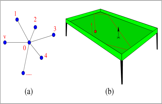
Figure 1: A star graph with $v$ edges (a) and a Šeba billiard (b).

2 Quantum star graphs

Star graphs are metric graphs of the type shown on Fig. 1 with a Schrödinger equation

$$-\frac{d^{2}}{dx_{j}^{2}}\Psi_{j}=k^{2}\Psi_{j},\quad x_{j}\in[0,L_{j}],$$ (3)

defined on the bonds and boundary conditions, for example

$$\Psi_{j}(0)=\Psi_{k}(0),$$ (4)

$$\sum_{j}\frac{\partial}{\partial x_{j}}\Psi_{j}(0)=0,$$ (5)

$$\frac{\partial}{\partial x_{j}}\Psi_{j}(L_{j})=0,$$ (6)

specified on the vertices. Here $L_{j}$ is the length of the $j$-th bond, $j=1\ldots v$, and the real variable $x_{j}$ varies from 0 to $L_{j}$, with 0 corresponding to the central vertex and $L_{j}$ to the outer vertex. The lengths $L_{j}$ are assumed to be incommensurate; see [12] for further details. We refer to positive values of the parameter $k$ for which the system (3)-(6) is solvable as eigenvalues of the quantum star graph.

Denoting the ordered sequence of eigenvalues by $\left\{k_{i}\right\}_{i=1}^{\infty}$, we define the spectral density by

$$d(k)=\sum_{i=1}^{\infty}\delta(k-k_{i}).$$ (7)

The statistic we shall mainly be concerned with is the two-point correlation function

$$R_{2}(x)=\frac{1}{\overline{d}^{2}}\left\langle d(k)d\left(k+\frac{x}{\overline{d}}\right)\right\rangle-\delta(x),$$ (8)

where $\overline{d}=\langle d(k)\rangle$ is the mean density, $\delta(x)$ is the Dirac $\delta$-function, and the average $\langle\ \cdot\ \rangle$ is either over $k$, or over the bond lengths $L_{j}$ (we shall specify which in each particular context). $R_{2}(x)$ is an even function and hence so is its Fourier transform,

$$K(\tau)=1+2\Re\int_{0}^{\infty}(R_{2}(x)-1)e^{2\pi ix\tau}d\tau,$$ (9)

which is called the form factor.

A complete series expansion of the $v\rightarrow\infty$ limit of $K(\tau)$ in powers of $\tau$ around $\tau=0$ was derived for the star graphs in [12] using the trace formula and a classification of the periodic orbits:

$$K(\tau)=\exp(-4\tau)+\sum_{j=2}^{\infty}\sum_{M=0}^{\infty}\frac{4^{j}}{j!}C_{j,M}\tau^{M+j+1},$$ (10)

where

$$C_{j,M}=(-2)^{M}\sum_{K=0}^{M}\frac{(K+j-1)!(M-K+j-1)!}{(M+j-1)!}F_{j}(K,M-K),$$ (11)

with

$$F_{1}(K,N)=\frac{\binom{K+N}{N}}{(N+1)!(K+1)!},$$ (12)

and

$$F_{j}(K,N)=\sum_{k=0}^{K}\sum_{n=0}^{N}F_{1}(k,n)F_{j-1}(K-k,N-n).$$ (13)

Explicitly,

$$K(\tau)=e^{-4\tau}+8\tau^{3}-\frac{32}{3}\tau^{4}+\frac{16}{3}\tau^{5}-\frac{128}{15}\tau^{6}+\frac{16}{9}\tau^{7}+\frac{64}{63}\tau^{8}+o(\tau^{8}).$$ (14)

In this calculation, the average in (8) was over $k$. The result is in excellent agreement with the numerical data (see Fig. 2) but is limited by the fact that the radius of convergence of the series is finite, being approximately $0.63$ (found by applying Cauchy’s test to the coefficients in the series, but see also Fig. 2). The range of convergence can be extended using Padé approximation (again, see Fig. 2), which suggests that the singularity causing the divergence is not on the positive real line [16].

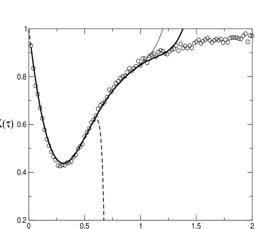
Figure 2: The sum of the first 30 terms in the expansion (10) (dashed line), which converges in the range $\tau\leq\tau^{*}\approx 0.63$, compared to the results of a numerical computation [8] of $K(\tau)$ (circles). Also shown are the Padé approximations to the series of order $[21/20]$ (thin solid line) and $[23/23]$ (thick solid line).

Here we approach the problem from a different direction: it is possible to solve equations (3)-(6) to derive an explicit condition on $k$ to be an eigenvalue. Indeed, the general solution of (3) on a star graph can be written in the form $\Psi_{j}(x)=A_{j}\cos(k(x+\phi_{j}))$, $j=1,\ldots,v$. Applying condition (6), we obtain $\phi_{j}=-L_{j}$ while condition (4) on the central vertex implies $A_{j}\cos(L_{j}k)=\mbox{const}$. Finally, applying condition (5) and dividing by $A_{j}\cos(L_{j}k)$ we obtain

$$\sum_{j=1}^{v}\tan{L_{j}k}=0.$$ (15)

Similar expressions can easily be found when different boundary conditions are applied at the central vertex. The general equation reads

$$\sum_{j=1}^{v}\tan{L_{j}k}=\frac{1}{\lambda},$$ (16)

where $\lambda$ is arbitrary parameter. However, in the limit as $v\to\infty$, $\lambda$ fixed, the two-point correlation function turns out to be independent of $\lambda$ (see the comment following equation (49)). Our calculations will therefore be performed for $\lambda^{-1}=0$.

Note the similarity between (16) and the quantization condition (1) for Šeba billiards when $|\psi_{n}({\bf x_{0}})|^{2}={\rm constant}$.

Condition (15) means that $k$ is an eigenvalue if and only if it is a zero of the function $F(k)=\sum_{j=1}^{v}\tan L_{j}k$, and so we can express the density $d(k)$ as

$$d(k)=\frac{1}{2\pi}\int|F^{\prime}(k)|e^{izF(k)}dz=\frac{1}{2\pi}\int\sum_{s=1}^{v}\frac{L_{s}}{\cos^{2}{L_{s}k}}e^{iz\sum_{j=1}^{v}\tan{L_{j}k}}dz.$$ (17)

Our analysis of the spectral correlations will be based on this representation.

3 Mean density.

As an example of the techniques to be employed later, we begin by calculating the mean density $\overline{d}$ defined as

$$\overline{d}=\lim_{\Delta L\to 0,{k\to\infty}}\Big{\langle}d(k)\Big{\rangle}_{\left\{L_{j}\right\}}$$ (18)

where now the average is with respect to the individual lengths of the bonds, rather than over $k$:

$$\langle\ \cdot\ \rangle_{\left\{L_{j}\right\}}=\int_{L_{0}}^{L_{0}+\Delta L}\cdots\int_{L_{0}}^{L_{0}+\Delta L}\cdot\hskip 14.22636pt\frac{dL_{1}}{\Delta L}\cdots\frac{dL_{v}}{\Delta L}.$$ (19)

That is, we assume that the lengths are independent random variables distributed uniformly on the interval $[L_{0},L_{0}+\Delta L]$. We also assume that $\Delta L$ and $k$ tend to their respective limits in such a way that $\Delta Lk\to\infty$.

Applying this averaging to (17) we obtain

$$\Big{\langle}d(k)\Big{\rangle}_{\left\{L_{j}\right\}} = \frac{1}{2\pi}\int_{-\infty}^{\infty}dz\sum_{s=1}^{v}\int\cdots\int_{L_{0}}^{L_{0}+\Delta L}L_{s}\frac{e^{iz\sum_{j=1}^{v}\tan{kL_{j}}}}{\cos^{2}{kL_{s}}}\frac{dL_{1}}{\Delta L}\cdots\frac{dL_{v}}{\Delta L}$$ (20)

$$= \frac{v}{2\pi}\int_{-\infty}^{\infty}dz\left(\int_{L_{0}}^{L_{0}+\Delta L}e^{iz\tan{kL}}\frac{dL}{\Delta L}\right)^{v-1}\left(\int_{L_{0}}^{L_{0}+\Delta L}L\frac{e^{iz\tan{kL}}}{\cos^{2}{kL}}\frac{dL}{\Delta L}\right)$$

$$\equiv \frac{v}{2\pi}\int_{-\infty}^{\infty}{\tilde{f}}^{v-1}(z){\tilde{g}}(z)\ dz.$$

Here

$${\tilde{g}}(z)=\int_{L_{0}}^{L_{0}+\Delta L}L\frac{e^{iz\tan{kL}}}{\cos^{2}{kL}}\frac{dL}{\Delta L}\approx\frac{L_{0}}{\Delta Lk}\int_{\tan{kL_{0}}}^{\tan{k(L_{0}+\Delta L)}}e^{iz\tan{kL}}\ d\tan{kL},$$ (21)

where we were able to approximate $L$ by $L_{0}$ because it is slowly varying (compared with $\tan{kL}$) and ultimately we will take the limit $\Delta L\to 0$. Now, since $\tan{kL}$ is a periodic function with the period of $\pi/k$, and the integration is performed over the interval containing approximately $\Delta Lk/\pi$ periods, we can further approximate

$${\tilde{g}}(z) = \frac{L_{0}}{\Delta Lk}\left(\frac{\Delta Lk}{\pi}\int_{-\infty}^{\infty}e^{iz\tan{kL}}\ d\tan{kL}+O(1)\right)$$ (22)

$$\approx 2L_{0}\delta(z),$$

where $O(1)$ is a quantity which is bounded as $k\Delta L\to\infty$. Similarly,

$${\tilde{f}}(z) = \int_{L_{0}}^{L_{0}+\Delta L}e^{iz\tan{kL}}\frac{dL}{\Delta L}=\frac{L_{0}}{\Delta Lk}\int_{\tan{kL_{0}}}^{\tan{k(L_{0}+\Delta L)}}e^{iz\tan{kL}}\frac{d\tan{kL}}{1+\tan^{2}{kL}}$$ (23)

$$\approx \frac{1}{\pi}\int_{-\infty}^{\infty}\frac{e^{iz\alpha}}{1+\alpha^{2}}d\alpha=e^{-|z|},$$

where the last integral was evaluated by closing the contour in either the upper ($z>0$) or lower ($z<0$) half-plane.

Substituting the results into (20) we obtain for the average density

$$\overline{d}=\frac{v}{2\pi}2L_{0}\int_{-\infty}^{\infty}e^{-(v-1)|z|}\delta(z)dz=\frac{L_{0}v}{\pi},$$ (24)

which coincides with the result of averaging over $k$ with the bond-lengths fixed [7, 8, 12].

4 Two-point correlation function

The two-point correlation function is given by

$$R_{2}(x)=\lim_{\Delta L\to 0,k\to\infty}\frac{1}{{\overline{d}}^{2}}R\left(k,k+\frac{x}{\overline{d}}\right),$$ (25)

where $\overline{d}$ is the mean density, the limit is taken in such a way that $k\Delta L\to\infty$, and we take

$$R(k_{1},k_{2}) = \langle d(k_{1})d(k_{2})\rangle_{\left\{L_{j}\right\}}$$

$$= \left\langle\int_{-\infty}^{\infty}\sum_{r,s=1}^{v}\frac{L_{r}L_{s}e^{i\sum_{j=1}^{v}(z_{1}\tan{k_{1}L_{j}}+z_{2}\tan{k_{2}L_{j}})}}{\cos^{2}k_{1}L_{r}\cos^{2}k_{2}L_{s}}\frac{d{\bf z}}{4\pi^{2}}\right\rangle_{\left\{L_{j}\right\}},$$

with ${\bf z}=(z_{1},z_{2})$.

In this case, the analogue of (20) is that

$$R(k_{1},k_{2})=\int_{-\infty}^{\infty}\left\{vg({\bf z})f^{v-1}({\bf z})+v(v-1)\phi_{1}({\bf z})\phi_{2}({\bf z})f^{v-2}({\bf z})\right\}\frac{d{\bf z}}{4\pi^{2}},$$ (27)

where

$$f({\bf z}) = \frac{1}{\Delta L}\int_{L_{0}}^{L_{0}+\Delta L}e^{i(z_{1}\tan(k_{1}L)+z_{2}\tan(k_{2}L))}dL,$$ (28)

$$g({\bf z}) = \frac{1}{\Delta L}\int_{L_{0}}^{L_{0}+\Delta L}\frac{L^{2}}{\cos^{2}k_{1}L\cos^{2}k_{2}L}e^{i(z_{1}\tan(k_{1}L)+z_{2}\tan(k_{2}L))}dL,$$ (29)

$$\phi_{1}({\bf z}) = \frac{1}{\Delta L}\int_{L_{0}}^{L_{0}+\Delta L}\frac{L}{\cos^{2}k_{1}L}e^{i(z_{1}\tan(k_{1}L)+z_{2}\tan(k_{2}L))}dL,$$ (30)

$$\phi_{2}({\bf z}) = \frac{1}{\Delta L}\int_{L_{0}}^{L_{0}+\Delta L}\frac{L}{\cos^{2}k_{2}L}e^{i(z_{1}\tan(k_{1}L)+z_{2}\tan(k_{2}L))}dL.$$ (31)

Substituting $k_{1}=k$, $k_{2}=k+\pi x/(vL_{0})$, where $x$ is fixed, and taking the limits $k\to\infty$, $\Delta L\to 0$ (while $k\Delta L\to\infty$), we obtain for the first integral

$$f({\bf z}) = \frac{1}{\Delta L}\int_{L_{0}}^{L_{0}+\Delta L}e^{i\left(z_{1}\tan(kL)+z_{2}\tan\left(kL+\frac{\pi xL}{vL_{0}}\right)\right)}dL$$ (32)

$$\approx \frac{1}{\pi}\int_{-\pi/2}^{\pi/2}e^{i\left(z_{1}\tan\phi+z_{2}\tan\left(\phi+\frac{\pi x}{v}\right)\right)}d\phi,$$

where we have again used $L/L_{0}\approx 1$ and, as in the transition from (21) to (22), we have approximated $f$ by the integral over one period. We now write

$$\tan\left(\phi+\frac{\pi x}{v}\right)=\frac{\tan\phi+\tan\left(\frac{\pi x}{v}\right)}{1-\tan\phi\tan\left(\frac{\pi x}{v}\right)}=-\beta+\frac{1+\beta^{2}}{\beta-\tan\phi},$$ (33)

where $\beta=(\tan(\pi x/v))^{-1}\propto v/(\pi x)$ (we are interested in the $v\to\infty$ limit). Performing the change of variables $\alpha=\tan\phi-\beta$, we arrive at

$$f({\bf z})\approx\frac{e^{i\beta(z_{1}-z_{2})}}{\pi}\int_{-\infty}^{\infty}e^{iz_{1}\alpha-iz_{2}\frac{\beta^{2}+1}{\alpha}}\frac{d\alpha}{(\alpha+\beta)^{2}+1}.$$ (34)

Note that $f({\bf z})$ is invariant under the exchange $z_{1}\leftrightarrow z_{2}$ and $\beta\to-\beta$, which can be verified by the change of variables $\alpha=(\beta^{2}+1)/y$ in (34).

To evaluate the integral in (34) we differentiate it with respect to $z_{1}$ and $z_{2}$ to get

$$\frac{\partial f}{\partial z_{1}}-\frac{\partial f}{\partial z_{2}}\! = \!\frac{ie^{i\beta(z_{1}-z_{2})}}{\pi}\int_{-\infty}^{\infty}e^{iz_{1}\alpha-iz_{2}\frac{\beta^{2}+1}{\alpha}}\left(2\beta+\alpha+\frac{\beta^{2}+1}{\alpha}\right)\frac{d\alpha}{(\alpha+\beta)^{2}+1}$$ (35)

$$= \!\frac{ie^{i\beta(z_{1}-z_{2})}}{\pi}\int_{-\infty}^{\infty}e^{iz_{1}\alpha-iz_{2}\frac{\beta^{2}+1}{\alpha}}\frac{d\alpha}{\alpha}=-e^{i\beta(z_{1}-z_{2})}\Phi(z_{1},z_{2}),$$

where

$$\Phi(z_{1},z_{2}) \equiv -\frac{i}{\pi}\int_{-\infty}^{\infty}e^{iz_{1}\alpha-iz_{2}\frac{\beta^{2}+1}{\alpha}}\frac{d\alpha}{\alpha}$$

$$= 2\mathop{\rm sign}\nolimits(z_{1})H(-z_{1}z_{2})J_{0}\left(2\sqrt{-(\beta^{2}+1)z_{1}z_{2}}\right),$$

$J_{0}(x)$ being the Bessel function of the first kind and $H(x)$ the Heaviside function (characteristic function of the half axis $[0,\infty)$).

Applying the method of characteristics to the PDE

$$\frac{\partial f}{\partial z_{1}}-\frac{\partial f}{\partial z_{2}}=-e^{i\beta(z_{1}-z_{2})}\Phi(z_{1},z_{2}),$$ (37)

we obtain the solution

$$f({\bf z})=e^{-|z_{1}+z_{2}|}-\int_{0}^{z_{1}}e^{i\beta(2y-z_{1}-z_{2})}\Phi\left(y,z_{1}+z_{2}-y\right)dy.$$ (38)

Treating the integral for $g({\bf z})$ (see (29)) in a fashion similar to the one used to obtain (34) leads us to

$$g(z_{1},z_{2}) \approx \frac{L_{0}^{2}}{\pi}\int_{-\pi/2}^{\pi/2}\frac{e^{i(z_{1}\tan(\phi)+z_{2}\tan(\phi+\pi x/v))}}{\cos^{2}(\phi)\cos^{2}(\phi+\pi x/v)}d\phi$$

$$= L_{0}^{2}\frac{e^{i\beta(z_{1}-z_{2})}}{\pi}\int_{-\infty}^{\infty}e^{iz_{1}\alpha-iz_{2}\frac{\beta^{2}+1}{\alpha}}\left(1+\left(\frac{1+\beta^{2}}{\alpha}+\beta\right)^{2}\right)d\alpha.$$

Comparing this integral to the one in (4), and noting that

$$1+\left(\frac{1+\beta^{2}}{\alpha}+\beta\right)^{2}=\frac{\beta^{2}+1}{\alpha}\left(\alpha+\beta+\frac{\beta^{2}+1}{\alpha}+\beta\right),$$ (40)

we have that

$$g({\bf z})=L_{0}^{2}(\beta^{2}+1)\left(\frac{\partial}{\partial z_{1}}-\frac{\partial}{\partial z_{2}}\right)\left[e^{i\beta(z_{1}-z_{2})}\Phi(z_{1},z_{2})\right].$$ (41)

One can derive a similar expression for the functions $\phi_{1}({\bf z})$,

$$\phi_{1}({\bf z})\approx L_{0}\frac{e^{i\beta(z_{1}-z_{2})}}{\pi}\int_{-\infty}^{\infty}e^{iz_{1}\alpha-iz_{2}\frac{\beta^{2}+1}{\alpha}}d\alpha=L_{0}e^{i\beta(z_{1}-z_{2})}\frac{\partial}{\partial z_{1}}\Phi(z_{1},z_{2}),$$ (42)

and $\phi_{2}({\bf z})$,

$$\phi_{2}({\bf z}) \approx L_{0}\frac{e^{i\beta(z_{1}-z_{2})}}{\pi}\int_{-\infty}^{\infty}e^{iz_{1}\alpha-iz_{2}\frac{\beta^{2}+1}{\alpha}}\frac{(\beta^{2}+1)d\alpha}{\alpha^{2}}$$ (43)

$$= -L_{0}e^{i\beta(z_{1}-z_{2})}\frac{\partial}{\partial z_{2}}\Phi(z_{1},z_{2}).$$

Now we have all the ingredients necessary for evaluating the integral in (27). Substituting the expression for $g({\bf z})$, (41), into the first half of the integral and integrating it by parts we obtain

$$\int\frac{d{\bf z}}{4\pi^{2}}vf^{v-1}g = vL_{0}^{2}\int\frac{d{\bf z}}{4\pi^{2}}f^{v-1}(\beta^{2}+1)\left(\frac{\partial}{\partial z_{1}}-\frac{\partial}{\partial z_{2}}\right)\left[e^{i\beta(z_{1}-z_{2})}\Phi\right]$$ (44)

$$= -vL_{0}^{2}\int\frac{d{\bf z}}{4\pi^{2}}(\beta^{2}+1)e^{i\beta(z_{1}-z_{2})}\Phi\left(\frac{\partial}{\partial z_{1}}-\frac{\partial}{\partial z_{2}}\right)\left[f^{v-1}({\bf z})\right]$$

$$= v(v-1)L_{0}^{2}\int\frac{d{\bf z}}{4\pi^{2}}(\beta^{2}+1)f^{v-2}e^{2i\beta(z_{1}-z_{2})}\Phi^{2}.$$

Thus

$$R_{2}(x)=\frac{v(v-1)L_{0}^{2}}{\overline{d}^{2}}\int\frac{d{\bf z}}{4\pi^{2}}f^{v-2}e^{2i\beta(z_{1}-z_{2})}\left[(\beta^{2}+1)\Phi^{2}-\frac{\partial\Phi}{\partial z_{1}}\frac{\partial\Phi}{\partial z_{2}}\right].$$ (45)

Now we need to take the limit $v\to\infty$. To do so we write $f^{v-2}({\bf z})=e^{(v-2)\ln f}$ and rescale $f({\bf z})$

$$f({\bf u}/\beta)=e^{-\frac{|u_{1}+u_{2}|}{\beta}}-\frac{1}{\beta}\int_{0}^{u_{1}}e^{i(2y-u_{1}-u_{2})}\Psi(y,u_{1}+u_{2}-y)dy,$$ (46)

and hence, to the leading order in $1/\beta=\pi x/v$, we have

$$(v-2)\ln f({\bf u}) \approx -\pi x\left(|u_{1}+u_{2}|+\int_{0}^{u_{1}}e^{i(2y-u_{1}-u_{2})}\Psi(y,u_{1}+u_{2}-y)dy\right)$$ (47)

$$\equiv -\pi xQ,$$

where $\Psi$ is the rescaled function $\Phi$,

$$\Psi({\bf u})=\Phi\left(\frac{{\bf u}}{\beta}\right)=2\mathop{\rm sign}\nolimits(u_{1})H(-u_{1}u_{2})J_{0}\left(2\sqrt{-u_{1}u_{2}}\right),$$ (48)

and we have taken the limit $v\to\infty$ ($\beta\to\infty$).

Renormalizing the rest of (45) and taking the limit $v\to\infty$ we obtain

$$R_{2}(x)=\frac{1}{4}\int d{\bf u}e^{-\pi xQ}e^{2i(u_{1}-u_{2})}\left[\Psi^{2}-\frac{\partial\Psi}{\partial u_{1}}\frac{\partial\Psi}{\partial u_{2}}\right].$$ (49)

The only change when the above calculation is generalized to other boundary conditions at the central vertex (i.e. to nonzero values of $\lambda^{-1}$ in (16)) is the appearance of a factor $e^{-\lambda^{-1}(z_{1}+z_{2})}$ next to every occurrence of $d{\bf z}$ in the above integrals. For $\lambda$ fixed, this factor disappears after rescaling ${\bf z}={\bf u}/\beta$ and taking the limit $\beta\to\infty$. Hence equation (49) is then independent of $\lambda$. In the case when $\lambda^{-1}={\tilde{\lambda}}^{-1}v$, the dependence of the spectral statistics on the boundary conditions at the central vertex persists. The above expressions then coincide with those for those for Šeba billiards with a renormalized coupling consant, given in [15].

For the derivatives of the function $\Psi$ one has

$$\frac{\partial\Psi}{\partial u_{1}} = 2\left(J_{0}(0)\delta(u_{1})+\mathop{\rm sign}\nolimits(u_{1})H(-u_{1}u_{2})\frac{u_{2}J^{\prime}_{0}\left(2\sqrt{-u_{1}u_{2}}\right)}{\sqrt{-u_{1}u_{2}}}\right),$$ (50)

$$\frac{\partial\Psi}{\partial u_{2}} = 2\left(-J_{0}(0)\delta(u_{2})+\mathop{\rm sign}\nolimits(u_{1})H(-u_{1}u_{2})\frac{u_{1}J^{\prime}_{0}\left(2\sqrt{-u_{1}u_{2}}\right)}{\sqrt{-u_{1}u_{2}}}\right),$$ (51)

therefore, using $J_{0}(0)=1$ and $J^{\prime}_{0}(x)=-J_{1}(x)$,

$$\frac{\partial\Psi}{\partial u_{1}}\frac{\partial\Psi}{\partial u_{2}}=-4\left(\delta(u_{1})\delta(u_{2})+H(-u_{1}u_{2})J_{1}^{2}\left(2\sqrt{-u_{1}u_{2}}\right)\right).$$ (52)

Thus

$$R_{2}(x)=1+\!\!\int\!\!e^{-\pi xQ+2i(u_{1}-u_{2})}\left[J_{0}^{2}\left(2\sqrt{-u_{1}u_{2}}\right)+J_{1}^{2}\left(2\sqrt{-u_{1}u_{2}}\right)\right]\!H(-u_{1}u_{2})d{\bf u}.$$ (53)

Now we perform the change of variables $u_{2}\mapsto-u_{2}$ arriving at the following integral representation of the two-point correlation function,

$$R_{2}(x)=1+\int_{D}e^{-\pi xM({\bf u})+2i(u_{1}+u_{2})}\left[J_{0}^{2}\left(2\sqrt{u_{1}u_{2}}\right)+J_{1}^{2}\left(2\sqrt{u_{1}u_{2}}\right)\right]d{\bf u}.$$ (54)

Here the domain of integration $D$ includes first and third quadrants of the $u_{1}u_{2}$-plane and $M({\bf u})$ is given by

$$M({\bf u}) \equiv M(u_{1},u_{2})=|u_{1}-u_{2}|+\int_{0}^{u_{1}}e^{i(2y-u_{1}+u_{2})}\Psi(y,u_{1}-u_{2}-y)dy$$ (55)

$$= |u_{1}|+|u_{2}|-2i\mathop{\rm sign}\nolimits(u_{1})\sum_{r,s=1}^{\infty}\frac{(iu_{1})^{r}(iu_{2})^{s}(r+s-2)!}{r!s!(r-1)!(s-1)!}.$$

Equation (54) constitutes an exact formula for $R_{2}(x)$ for star graphs in the limit $v\rightarrow\infty$. It is our main result. The point we seek to draw attention to is that it is exactly the same as the one obtained in [15] for Šeba billiards when $|\psi_{n}({\bf x_{0}})|^{2}={\rm constant}$ in (2) and $\lambda\rightarrow\infty$. We will expand on this observation later. First, we consider some of the properties of the two-point correlation function and the form factor in more detail.

5 Expansion for large $x$

To derive an expansion of the two point correlation function $R_{2}(x)$ for large $x$ we notice that since $M(-{\bf u})=\overline{M({\bf u})}$, the integral over the third quadrant in (54) is equal to the complex conjugate of the integral over second quarter-plane, i.e.

$$R_{2}(x)=1+2\Re\int\!\!\int_{0}^{\infty}e^{-\pi xM({\bf u})+2i(u_{1}+u_{2})}J({\bf u})d{\bf u},$$ (56)

where

$$J({\bf u})=J_{0}^{2}(2\sqrt{u_{1}u_{2}})+J_{1}^{2}(2\sqrt{u_{1}u_{2}})=\sum_{n=0}^{\infty}\frac{(-1)^{n}u_{1}^{n}u_{2}^{n}(2n)!}{(n+1)!(n!)^{3}}.$$ (57)

Now we can use the expansion of $M({\bf u})$, (55), to expand $R_{2}(x)$ in the powers of $1/x$. We substitute $u_{i}=\gamma_{i}/(x\pi)$ and obtain

$$R_{2}(x) = 1+2\Re\frac{1}{x^{2}\pi^{2}}\int\!\!\int_{0}^{\infty}d\gamma_{1}d\gamma_{2}e^{-\gamma_{1}-\gamma_{2}}\left[1+\frac{2i\left(\gamma_{1}+\gamma_{2}-\gamma_{1}\gamma_{2}\right)}{x\pi}\right.$$ (58)

$$-\left.\frac{\left(5\gamma_{1}\gamma_{2}+2\gamma_{1}^{2}+2\gamma_{2}^{2}-5\gamma_{1}\gamma_{2}^{2}-5\gamma_{1}^{2}\gamma_{2}+2\gamma_{1}^{2}\gamma_{2}^{2}\right)}{x^{2}\pi^{2}}+O\left(\frac{1}{x^{3}}\right)\right]$$

$$= 1+2\Re\left[\frac{1}{x^{2}\pi^{2}}+\frac{2i}{x^{3}\pi^{3}}-\frac{1}{x^{4}\pi^{4}}+\ldots\right].$$

To compare this to the expansion (14) of $K(\tau)$ we note that if $K(\tau)=1+\sum_{k=1}^{\infty}a_{k}\tau^{k}$ for $\tau>0$ then, inverting the Fourier transform in (9),

$$R_{2}(x)-1 = 2\Re\lim_{\epsilon\to 0}{\int_{0}^{\infty}(K(\tau)-1)e^{-2\pi i(x-i\epsilon)\tau}d\tau}$$ (59)

$$= 2\Re{\sum_{k=1}^{\infty}\left(\frac{-i}{2\pi}\right)^{k+1}\frac{a_{k}k!}{x^{k+1}}}.$$ (60)

Applying this to

$$K(\tau)=1-4\tau+8\tau^{2}-\frac{8}{3}\tau^{3}+O(\tau^{4}),$$ (61)

we see that the first few coefficients of the two expansions agree. The proof that it is so for all coefficients is given by the following proposition.

Proposition 1.

The asymptotic expansion (58) of the two-point correlation function and the expansion (10) of the form factor coincide under the Fourier transformation

$$\int\!\!\int_{0}^{\infty}e^{-\pi xM({\bf u})+2i(u_{1}+u_{2})}J({\bf u})d{\bf u}=\int_{0}^{\infty}\left(K(\tau^{\prime})-1\right)e^{-2\pi ix\tau^{\prime}}d\tau^{\prime}.$$ (62)

Proof.

The Fourier transform in (62) establishes the correspondence between the terms in the asymptotic expansion of

$$\widetilde{R_{2}}(x)=\int\!\!\int_{0}^{\infty}e^{-\pi xM({\bf u})+2i(u_{1}+u_{2})}J({\bf u})d{\bf u}$$ (63)

and the terms of the small $\tau$ expansion of $K(\tau)$. This correspondence is

$$\frac{1}{(2\pi ix)^{k}}\longleftrightarrow\frac{\tau^{k-1}}{(k-1)!}.$$ (64)

Our plan is to modify the integrand in the definition of $\widetilde{R_{2}}(x)$, getting rid of the factor $e^{2i(u_{1}+u_{2})}J({\bf u})$, expand the integral in inverse powers of $x$ and apply the correspondence rule (64) to recover (10).

First of all, as one can verify by direct substitution of the series for $M(u_{1},u_{2})$,

$$\left(\frac{\partial}{\partial\alpha_{1}}+\frac{\partial}{\partial\alpha_{2}}\right)\left(xM\left(\frac{\alpha_{1}}{x},\frac{\alpha_{2}}{x}\right)\right)=\sum_{r,s=0}^{\infty}i^{r+s}\binom{r+s}{r}\frac{(\alpha_{1}/x)^{r}(\alpha_{2}/x)^{s}}{r!s!}\\ =2e^{i(\alpha_{1}+\alpha_{2})/x}J_{0}\left(\frac{2\sqrt{\alpha_{1}\alpha_{2}}}{x}\right),$$ (65)

and

$$\frac{\partial}{\partial x}\left(xM\left(\frac{\alpha_{1}}{x},\frac{\alpha_{2}}{x}\right)\right)=\sum_{r,s=1}^{\infty}2i^{r+s+1}\frac{(r+s-1)!(\alpha_{1}/x)^{r}(\alpha_{2}/x)^{s}}{r!s!(r-1)!(s-1)!}\\ =-\frac{2i\sqrt{\alpha_{1}\alpha_{2}}}{x}J_{1}\left(\frac{2\sqrt{\alpha_{1}\alpha_{2}}}{x}\right)e^{i(\alpha_{1}+\alpha_{2})/x}.$$ (66)

Applying (66),

$$\frac{\partial^{2}}{\partial x^{2}}e^{-\pi xM\left(\frac{\alpha_{1}}{x},\frac{\alpha_{2}}{x}\right)}\\ =e^{-\pi xM}\left(-4\pi^{2}\frac{\alpha_{1}\alpha_{2}}{x^{2}}J_{1}^{2}e^{2\phi}-\frac{2\pi i}{x^{3}}\left(2J_{0}e^{\phi}\alpha_{1}\alpha_{2}+iJ_{1}e^{\phi}\sqrt{\alpha_{1}\alpha_{2}}(\alpha_{1}+\alpha_{2})\right)\right),$$ (67)

where $\phi=i(\alpha_{1}+\alpha_{2})/x$ and for simplicity we have omitted the argument
$(\alpha_{1}/x,\alpha_{2}/x)$ of the functions $M$, $J_{0}$ and $J_{1}$.

Similarly, using (65), we have

$$\left(\frac{\partial}{\partial\alpha_{1}}+\frac{\partial}{\partial\alpha_{2}}\right)^{2}e^{-\pi xM\left(\frac{\alpha_{1}}{x},\frac{\alpha_{2}}{x}\right)}\\ =e^{-\pi xM}\left(4\pi^{2}J_{0}^{2}e^{2\phi}-\frac{2\pi i}{\alpha_{1}\alpha_{2}x}\left(2J_{0}e^{\phi}\alpha_{1}\alpha_{2}+iJ_{1}e^{\phi}\sqrt{\alpha_{1}\alpha_{2}}(\alpha_{1}+\alpha_{2})\right)\right).$$ (68)

Noticing the similarity between (67) and (68), we subtract the first from the second, with the appropriate factors, to obtain

$$\frac{1}{4\pi^{2}}\left[\frac{1}{x^{2}}\left(\frac{\partial}{\partial\alpha_{1}}+\frac{\partial}{\partial\alpha_{2}}\right)^{2}-\frac{1}{\alpha_{1}\alpha_{2}}\frac{\partial^{2}}{\partial x^{2}}\right]e^{-\pi xM\left(\frac{\alpha_{1}}{x},\frac{\alpha_{2}}{x}\right)}\\ =\frac{1}{x^{2}}\left[J_{0}^{2}+J_{1}^{2}\right]e^{2\phi}e^{-xM},$$ (69)

where, as before, the argument $(\alpha_{1}/x,\alpha_{2}/x)$ of $M$, $J_{0}$ and $J_{1}$ has been omitted. The right hand side of (69) is exactly the integrand of (56) if we perform the change of variables $u_{i}=\alpha_{i}/x$ and, therefore,

$$\widetilde{R_{2}}(x)=\iint_{0}^{\infty}\frac{d\alpha_{1}d\alpha_{2}}{4\pi^{2}}\left[\frac{1}{x^{2}}\left(\frac{\partial}{\partial\alpha_{1}}+\frac{\partial}{\partial\alpha_{2}}\right)^{2}-\frac{1}{\alpha_{1}\alpha_{2}}\frac{\partial^{2}}{\partial x^{2}}\right]e^{-\pi xM\left(\frac{\alpha_{1}}{x},\frac{\alpha_{2}}{x}\right)}.$$ (70)

The first term in the integral can be evaluated as follows,

$$\iint_{0}^{\infty}\frac{d\alpha_{1}d\alpha_{2}}{4\pi^{2}x^{2}}\left(\frac{\partial}{\partial\alpha_{1}}+\frac{\partial}{\partial\alpha_{2}}\right)^{2}e^{-\pi xM\left(\frac{\alpha_{1}}{x},\frac{\alpha_{2}}{x}\right)}\\ =\left(-\int_{0}^{\infty}\frac{d\alpha_{2}}{4\pi x^{2}}\left[\Theta\right]_{\alpha_{1}=0}^{\infty}-\int_{0}^{\infty}\frac{d\alpha_{1}}{2\pi x^{2}}\left[\Theta\right]_{\alpha_{2}=0}^{\infty}\right),$$ (71)

where

$$\Theta=\left(\frac{\partial}{\partial\alpha_{1}}+\frac{\partial}{\partial\alpha_{2}}\right)e^{-\pi xM\left(\frac{\alpha_{1}}{x},\frac{\alpha_{2}}{x}\right)}=2e^{i(\alpha_{1}+\alpha_{2})/x}J_{0}\left(\frac{2\sqrt{\alpha_{1}\alpha_{2}}}{x}\right)e^{-\pi xM}.$$ (72)

Since

$$\left[\Theta\right]_{\alpha_{1}=0}^{\infty}=-2e^{i\alpha_{2}/x}e^{-\pi\alpha_{2}},\qquad\left[\Theta\right]_{\alpha_{2}=0}^{\infty}=-2e^{i\alpha_{1}/x}e^{-\pi\alpha_{1}},$$ (73)

we obtain

$$\iint_{0}^{\infty}\frac{d\alpha_{1}d\alpha_{2}}{4\pi^{2}x^{2}}\left(\frac{\partial}{\partial\alpha_{1}}+\frac{\partial}{\partial\alpha_{2}}\right)^{2}e^{-\pi xM\left(\frac{\alpha_{1}}{x},\frac{\alpha_{2}}{x}\right)}=\frac{1}{2\pi x^{2}}\frac{2}{\pi-i/x}.$$ (74)

Now we can expand the result in inverse powers of $x$ and apply the correspondence rule (64). We obtain

$$\frac{1}{\pi x}\frac{1}{\pi x-i}=-\sum_{k=0}^{\infty}\left(\frac{i}{\pi x}\right)^{k+2}\longleftrightarrow 2\sum_{k=0}^{\infty}\frac{(-2\tau)^{k+1}}{(k-1)!}=2\left(e^{-2\tau}-1\right).$$ (75)

Next we need to expand the second part of the integrand in (70),

$$\frac{\partial^{2}}{\partial x^{2}}e^{-\pi xM}=\frac{\partial^{2}}{\partial x^{2}}e^{-\pi(\alpha_{1}+\alpha_{2})}\exp\left(2\pi i\sum_{r,s=0}^{\infty}\frac{(i\alpha_{1})^{r+1}(i\alpha_{2})^{s+1}(r+s)!}{x^{r+s+1}r!s!(r+1)!(s+1)!}\right)\\ =e^{-\pi(\alpha_{1}+\alpha_{2})}\frac{\partial^{2}}{\partial x^{2}}\left[\sum_{j=0}^{\infty}\frac{(2\pi i)^{j}}{j!}\left(\sum_{r,s=0}^{\infty}\frac{(i\alpha_{1})^{r+1}(i\alpha_{2})^{s+1}(r+s)!}{x^{r+s+1}r!s!(r+1)!(s+1)!}\right)^{j}\right].$$ (76)

Using the same notation as in (12),

$$\left(\sum_{r,s=0}^{\infty}\frac{(i\alpha_{1})^{r+1}(i\alpha_{2})^{s+1}(r+s)!}{x^{r+s+1}r!s!(r+1)!(s+1)!}\right)^{j}=\left(\sum_{r,s=0}^{\infty}\frac{(i\alpha_{1})^{r+1}(i\alpha_{2})^{s+1}}{x^{r+s+1}}F_{1}(r,s)\right)^{j}\\ =\sum_{R,S=0}^{\infty}\frac{(i\alpha_{1})^{R+j}(i\alpha_{2})^{S+j}}{x^{R+S+j}}F_{j}(R,S),$$ (77)

where, as before, $F_{j}(R,S)$ is the $j$th convolution of $F_{1}(R,S)$ with itself. Thus

$$\frac{\partial^{2}}{\partial x^{2}}e^{-\pi xM\left(\frac{\alpha_{1}}{x},\frac{\alpha_{2}}{x}\right)}=e^{-\pi(\alpha_{1}+\alpha_{2})}\sum_{j=1}^{\infty}\frac{(2\pi i)^{j}}{j!}\\ \times\sum_{R,S=0}^{\infty}\frac{(R+S+j-1)!(i\alpha_{1})^{R+j}(i\alpha_{2})^{S+j}}{(R+S+j+1)!x^{R+S+j+2}}F_{j}(R,S).$$ (78)

Finally we integrate against $d\alpha_{1}d\alpha_{2}/(4\pi^{2}\alpha_{1}\alpha_{2})$ to arrive at

$$-\iint_{0}^{\infty}\frac{d\alpha_{1}d\alpha_{2}}{4\pi^{2}\alpha_{1}\alpha_{2}}\frac{\partial^{2}}{\partial x^{2}}e^{-\pi xM\left(\frac{\alpha_{1}}{x},\frac{\alpha_{2}}{x}\right)}\\ =-\sum_{j=1}^{\infty}\frac{(2\pi i)^{j}}{4\pi^{2}j!}\sum_{R,S=0}^{\infty}\frac{(R+S+j+1)!(R+j-1)!(S+j-1)!}{(R+S+j-1)!(-i\pi)^{R+S+2j}x^{R+S+j+2}}F_{j}(R,S)\\ \longleftrightarrow\tau\sum_{j=1}^{\infty}\frac{(4\tau)^{j}}{j!}\sum_{R,S=0}^{\infty}\frac{(-2\tau)^{R+S}(R+j-1)!(S+j-1)!}{(R+S+j-1)!}F_{j}(R,S).$$ (79)

This is exactly the same as the $j$ sum in (10) with the exception of the extra $j=1$ term in the summation above. For $j=1$ we have

$$4\tau^{2}\sum_{R,S=0}^{\infty}\frac{(-2\tau)^{R+S}R!S!}{(R+S)!}F_{j}(R,S)=\sum_{R,S=0}^{\infty}\frac{(-2\tau)^{R+S+2}}{(R+1)!(S+1)!}\\ =\left(\sum_{R=0}^{\infty}\frac{(-2\tau)^{R+1}}{(R+1)!}\right)\left(\sum_{S=0}^{\infty}\frac{(-2\tau)^{S+1}}{(S+1)!}\right)=(1-e^{-2\tau})^{2}\\ =1-2e^{-2\tau}+e^{-4\tau},$$ (80)

which, together with the terms $1$ and $2(e^{-2\tau}-1)$, gives the correct contribution $e^{-4\tau}$. ∎

6 Singularities of the form factor

One can also obtain some information about the singularities of $K(\tau)$ by Fourier transforming the integral representation (56). There is, however, a subtle problem associated with this approach. The form factor is by definition an even function defined on the real line. What we want to get from transforming (56) is an analytic function which coincides with the form factor for real $\tau>0$, so as to be able to study its complex singularities.

As we saw above,

$$\widetilde{R_{2}}(x)=\int\!\!\int_{0}^{\infty}e^{-\pi xM({\bf u})+2i(u_{1}+u_{2})}J({\bf u})d{\bf u}=\int_{0}^{\infty}(K(\tau^{\prime})-1)e^{-2\pi ix\tau^{\prime}}.$$ (81)

Integrating (81) against $e^{2\pi ix\tau}$ on the real line we obtain

$$\int_{-\infty}^{\infty}\widetilde{R_{2}}(x)e^{2\pi ix\tau}dx=K(\tau)-1,\qquad\tau>0.$$ (82)

One can check that this leads to the correct power series expansion of the form factor: give $x$ a small negative imaginary part, $x\mapsto x-i\epsilon$, in $\widetilde{R_{2}}(x)$ (this is consistent with (81)), substitute in the asymptotic expansion (56), and integrate term-by-term.

We now use $\widetilde{R_{2}}(-x)=\overline{\widetilde{R_{2}}(x)}$ to write

$$\int_{-\infty}^{\infty}e^{2\pi ix\tau}\widetilde{R_{2}}(x)dx=\int_{0}^{\infty}\left(e^{2\pi ix\tau}\widetilde{R_{2}}(x)+e^{-2\pi ix\tau}\overline{\widetilde{R_{2}}(x)}\right)dx.$$ (83)

The only factor $\widetilde{R_{2}}(x)$ which depends on $x$ is $e^{-\pi xM({\bf u})}$ and

$$\int_{0}^{\infty}e^{2\pi ix\tau}e^{-\pi xM({\bf u})}dx=\frac{1}{\pi(M({\bf u})-2i\tau)},$$ (84)

thus we have for the form factor

$$K(\tau)=1+\frac{1}{\pi}\int\!\!\int_{0}^{\infty}\left[\frac{e^{2i(u_{1}+u_{2})}}{M({\bf u})-2i\tau}+\frac{e^{-2i(u_{1}+u_{2})}}{\overline{M({\bf u})}+2i\tau}\right]J({\bf u})d{\bf u}.$$ (85)

The representation (85) presents us with a way to find the singularities of $K(\tau)$. These are given by the condition $\tau=M({\bf u}_{s})/(2i)$ and $\tau=\overline{M({\bf u}_{s})/(2i)}$, where the point ${\bf u}_{s}$ is such that

$$\frac{\partial M}{\partial u_{1}}({\bf u}_{s})=\frac{\partial M}{\partial u_{2}}({\bf u}_{s})=0.$$ (86)

The derivative with respect to $u_{2}$ is

$$\frac{\partial M}{\partial u_{2}}=1-2\int_{0}^{u_{1}}\left[e^{i(y+z)}J_{1}\left(2\sqrt{yz}\right)\sqrt{y/z}-ie^{i(y+z)}J_{0}\left(2\sqrt{yz}\right)\right]dy,$$ (87)

where $z=y-u_{1}+u_{2}$ and we have assumed that $u_{1}>u_{2}>0$. It is obvious from the expansion (55), however, that the function $M({\bf u})$ is continuously differentiable if $u_{1}u_{2}>0$ and hence that the expression (87) is valid for all $u_{1}>0$ and $u_{2}>0$. The integral in (87) is not easy to analyse and to simplify it we reduce our search to the line $u_{2}=u_{1}$, where

$$\frac{\partial M}{\partial u_{2}}(u_{2}=u_{1})=1-2\int_{0}^{u_{1}}e^{2iy}J_{1}(2y)dy+2i\int_{0}^{u_{1}}e^{2iy}J_{0}(2y)dy.$$ (88)

Performing the second integration by parts,

$$\int_{0}^{u_{1}}e^{2iy}J_{0}(2y)dy=\left.\frac{e^{2iy}J_{0}(2y)}{2i}\right|_{0}^{u_{1}}+\frac{2}{2i}\int_{0}^{u_{1}}e^{2iy}J_{1}(2y)dy,$$ (89)

we obtain, after simplification,

$$\frac{\partial M}{\partial u_{2}}(u_{2}=u_{1})=e^{2iu_{1}}J_{0}(2u_{1}).$$ (90)

Since $\frac{\partial M}{\partial u_{1}}(u_{2}=u_{1})=\frac{\partial M}{\partial u_{2}}(u_{2}=u_{1})$, we see that the zeros of the derivatives of $M({\bf u})$ on the line $u_{2}=u_{1}$ are given by the zeros of the Bessel function $J_{0}$. The nearest zero is at $u_{s}\approx 1.202$. Thus one of the singularities of $K(\tau)$ lies at $\tau_{s}=M(1.202,1.202)/(2i)=0.462-0.420i$. We note that $|\tau_{s}|=0.624$, which coincides with our previous numerical estimate of the radius of convergence of the series expansion of $K(\tau)$ in powers of $\tau$ around $\tau=0$. This strongly suggests that this singularity is the closest to the origin. To this end, we can prove the following.

Proposition 2.

Among the singularities arising from stationary points of$M(u_{1},u_{2})$ along the line $u_{2}=u_{1}$, the singularity at $\tau_{s}=M(1.202,1.202)/(2i)$ is the nearest to the origin.

Proof.

To show that the statement is true we need to prove that the function $|M(u,u)|^{2}$ is a nowhere decreasing function of $u$. On the line $u_{1}=u_{2}=u$ we have

$$M(u,u)=\int_{0}^{2u}e^{iy}J_{0}(y)dy=2e^{2iu}u\left(J_{0}(2u)-iJ_{1}(2u)\right).$$ (91)

Thus $|M(x/2,x/2)|^{2}=x^{2}\left(J_{0}^{2}(x)+J_{1}^{2}(x)\right)$ and its derivative is, after simplification, $\frac{d}{dx}|M(x/2,x/2)|^{2}=2xJ_{0}^{2}(x)\geq 0$. ∎

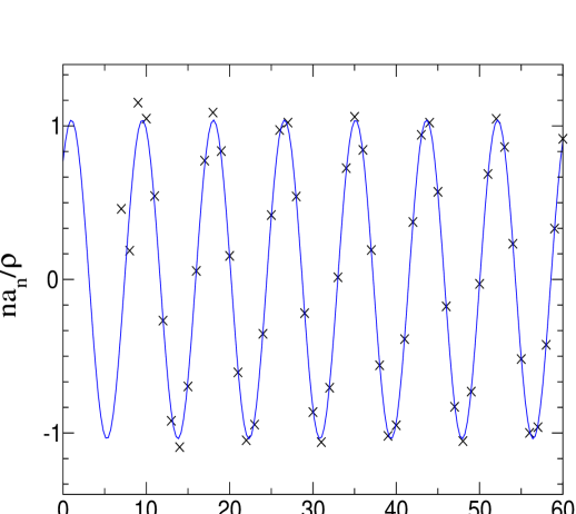
Figure 3: The coefficients of the power series expansion of $K(\tau)$ normalized by $\rho^{n}$ (crosses), compared to (95). As expected, the agreement improves as $n$ increases.

It is straightforward to approximate the behaviour of $K(\tau)$ near these singularities. We expand

$$M({\bf u}) \approx M({\bf u}_{s})+\frac{1}{2}\frac{\partial^{2}M}{\partial u_{1}^{2}}({\bf u}_{s})(u_{1}-u_{2})^{2}+\frac{1}{2}\frac{\partial^{2}M}{\partial u_{2}^{2}}({\bf u}_{s})(u_{2}-u_{s})^{2}$$ (92)

$$\qquad+\frac{\partial^{2}M}{\partial u_{1}\partial u_{2}}({\bf u}_{s})(u_{1}-u_{s})(u_{2}-u_{s})$$

$$= M({\bf u}_{s})+\alpha_{s}\left((u_{1}-u_{s})^{2}+(u_{2}-u_{s})^{2}\right).$$

For the singularity associated with the first Bessel zero, $\alpha_{s}\approx 0.385-0.349i$. Then, when $\tau$ is real,

$$K(\tau)\!\approx\!\frac{1}{\pi\alpha_{s}}\iint_{0}^{\infty}\frac{J({\bf u})e^{2i(u_{1}+u_{2})}d{\bf u}}{(u_{1}-u_{s})^{2}+(u_{2}-u_{s})^{2}+(M({\bf u}_{s})-2i\tau)/\alpha_{s}}+\mbox{c.c.}$$ (93)

The main contribution to the integral around these singularities is

$$K(\tau)\propto-C\ln\left(1-\frac{2i\tau}{M({\bf u}_{s})}\right)-\overline{C}\ln\left(1+\frac{2i\tau}{\overline{M({\bf u}_{s})}}\right),$$ (94)

where $C=J({\bf u}_{s})e^{4iu_{s}}/\alpha_{s}$. Expanding (94) into a series around $\tau=0$ we get

$$K(\tau)\propto 2\Re\left(C\sum_{n=1}^{\infty}\rho^{n}\frac{e^{i}n\phi}{n}\tau^{n}\right)=2A\sum_{n=1}^{\infty}\cos(\phi n+\psi)\frac{\rho^{n}}{n}\tau^{n},$$ (95)

where, for the singularity analysed above, $A=\left|J({\bf u}_{s})e^{4iu_{s}}/\alpha_{s}\right|\approx 0.519$, $\psi=\arg\left(J({\bf u}_{s})e^{4iu_{s}}/\alpha_{s}\right)\approx-0.737$, $\rho=|2i/M({\bf u}_{s})|\approx 1.602$ and $\phi=\arg\left(2i/M({\bf u}_{s})\right)\approx 0.737$. By Darboux’s Principle, the coefficients of the expansion (95) should comprise the leading contribution to large-order asymptotics of the exact coefficients given by (10) and (11). To compare them we plot the exact coefficients $na_{n}/\rho^{n}$ against the approximate coefficients $2A\cos(\phi n+\psi)$. The result is shown in Fig. 3.

7 Small $x$ limit of $R_{2}(x)$

Returning to (49), one can check that the function $\Psi$, defined by (48), satisfies the equation

$$\left[\frac{\partial^{2}}{2\partial u_{1}\partial u_{2}}+i\left(\frac{\partial}{\partial u_{1}}-\frac{\partial}{\partial u_{2}}\right)\right]\left(e^{2i(u_{1}-u_{2})}\Psi^{2}\right)\\ =e^{2i(u_{1}-u_{2})}\left(\frac{\partial\Psi}{\partial z_{1}}\frac{\partial\Psi}{\partial z_{2}}-\Psi^{2}\right).$$ (96)

Substituting it into (49) and integrating by parts we obtain

$$R_{2}(x)=-\frac{1}{4}\int d{\bf u}e^{-\pi xQ}\left[\frac{\partial^{2}}{2\partial u_{1}\partial u_{2}}+i\left(\frac{\partial}{\partial u_{1}}-\frac{\partial}{\partial u_{2}}\right)\right]\left(e^{2i(u_{1}-u_{2})}\Psi^{2}\right)\\ =\int\frac{d{\bf u}}{4}e^{2i(u_{1}-u_{2})}\Psi^{2}\left[i\left(\frac{\partial}{\partial u_{1}}-\frac{\partial}{\partial u_{2}}\right)-\frac{\partial^{2}}{2\partial u_{1}\partial u_{2}}\right]\left(e^{-\pi xQ}\right).$$ (97)

Now, using the identities

$$\frac{\partial Q}{\partial u_{1}}-\frac{\partial Q}{\partial u_{2}}=e^{i(u_{1}-u_{2})}\Psi,\qquad\frac{\partial^{2}Q}{2\partial u_{1}\partial u_{2}}=-ie^{i(u_{1}-u_{2})}\Psi,$$ (98)

which one can derive using the series expansion of $Q(u_{1},u_{2})=M(u_{1},-u_{2})$, we write

$$\left[i\left(\frac{\partial}{\partial u_{1}}-\frac{\partial}{\partial u_{2}}\right)-\frac{\partial^{2}}{2\partial u_{1}\partial u_{2}}\right]\left(e^{-\pi xQ}\right)\\ =e^{-\pi xQ}\left(-i\pi x\left(\frac{\partial Q}{\partial u_{1}}-\frac{\partial Q}{\partial u_{2}}\right)+\frac{\pi x}{2}\frac{\partial^{2}Q}{\partial u_{1}\partial u_{2}}-\frac{(\pi x)^{2}}{2}\frac{\partial Q}{\partial u_{1}}\frac{\partial Q}{\partial u_{2}}\right)\\ =-e^{-\pi xQ}\left(\frac{3i\pi x}{2}e^{i(u_{1}-u_{2})}\Psi+\frac{(\pi x)^{2}}{2}\frac{\partial Q}{\partial u_{1}}\frac{\partial Q}{\partial u_{2}}\right).$$ (99)

Thus we obtain, finally,

$$R_{2}(x)=-\int\frac{d{\bf u}}{8}e^{2i(u_{1}-u_{2})-\pi xQ}\Psi^{2}\left[\pi^{2}x^{2}\frac{\partial Q}{\partial u_{1}}\frac{\partial Q}{\partial u_{2}}+3i\pi x\Psi e^{i(u_{1}-u_{2})}\right].$$ (100)

From (100) one can see that the two-point correlation function $R_{2}(x)$ is linear in $x$ for small $x$. The slope was computed in [15]:

$$R_{2}(x)=\frac{\pi\sqrt{3}}{2}x+O(x^{2}).$$ (101)

8 Discussion

The derivation presented above provides a proof that two-point spectral correlations for certain Šeba billiards and quantum star graphs are the same, in the appropriate limits. This initially surprising fact has its explanation in the following observations. First, the dynamics in both systems is centered around a single point scatterer; in star graphs it is the central vertex, and in Šeba billiards the singularity. Furthermore, in between scatterings the dynamics is integrable in both cases.

Second, applying the Mittag-Leffler theorem to the meromorphic function $\tan z$, we have that

$$\tan z=\sum_{n=-\infty}^{\infty}\left(\frac{1}{n\pi+\pi/2-z}-\frac{1}{n\pi+\pi/2}\right).$$ (102)

We can therefore rewrite (16) in a form similar to (1) when $|\psi_{n}({\bf x_{0}})|^{2}={\rm constant}$. It thus becomes less surprising that the two point correlation functions of the two systems are the same, because in the limit $v\to\infty$ the poles in (15) have properties similar to those of a Poisson sequence.

Third, from the mathematical point of view star graphs and Šeba billiards are similar in that in both cases the scattering centre corresponds quantum mechanically to a perturbation of rank one.

Finally, we remark that our results demonstrate that, at least as regards the special case considered here, graphs are able to reproduce features of other, experimentally realizable, quantum systems, and also that they provide further confirmation that spectral statistics can be computed exactly using the trace formula when the periodic orbit statistics are known [12].

References

[1] M.V. Berry and M. Tabor, Proc. R. Soc. London A356 375 (1977).
[2] O. Bohigas, M.-J. Giannoni, and C. Schmit, Phys. Rev. Lett.52 1 (1984).
[3] M.V. Berry, Proc. R. Soc. London A400 229 (1985).