Parametric Evolution for a Deformed Cavity

Abstract

We consider a classically chaotic system that is described by a Hamiltonian ${\cal H}(Q,P;x)$, where $(Q,P)$ describes a particle moving inside a cavity, and $x$ controls a deformation of the boundary. The quantum-eigenstates of the system are $|n(x)\rangle$. We describe how the parametric kernel $P(n|m)=|\langle n(x)|m(x_{0})\rangle|^{2}$, also known as the local density of states, evolves as a function of $\delta x=x{-}x_{0}$. We illuminate the non-unitary nature of this parametric evolution, the emergence of non-perturbative features, the final non-universal saturation, and the limitations of random-wave considerations. The parametric evolution is demonstrated numerically for two distinct representative deformation processes.

I Introduction

A The local density of states

Consider a system that is described by an Hamiltonian ${\cal H}(Q,P;x)$ where $(Q,P)$ are canonical variables and $x$ is a constant parameter. Our interest in this paper is in the case where $(Q,P)$ describe the motion of a particle inside a cavity, and $x$ controls the deformation of the confining boundary. The 1D version of a cavity, also known as ‘potential well’, is illustrated in Fig.1. However, we are mainly interested in the case of chaotic cavities in $d>1$ dimensions. Cavities in $d=2$ dimensions, also known as billiard systems, are prototype examples in the studies of classical and quantum chaos, and we shall use them for the purpose of numerical illustrations.

FIG. 1.: The shape of a cavity in $d$ dimensions is defined by its $d-1$ boundary. The confining potential is $V(Q)$. The figure illustrates $V(Q)$ for 1D well. It also can be regarded as a cross section of $d>1$ cavity. The kinetic energy of the particle is $E=\mbox{$\frac{1}{2}$}mv^{2}$. The walls of the cavity exert a field of force $f$ on the bouncing particle. The hard wall limit corresponds to $f\rightarrow\infty$ and $V_{0}\rightarrow\infty$. For theoretical considerations it is convenient to assume that $f$ and $V_{0}$ are large but finite. Mathematically it is also convenient to think of the embedding space as having some huge but finite volume (not illustrated).

The eigenstates of the quantized Hamiltonian are $|n(x)\rangle$ and the corresponding eigen-energies are $E_{n}(x)$. The eigen-energies are assumed to be ordered, and the mean level spacing will be denoted by $\Delta$. We are interested in the parametric kernel

$$P(n|m)\ =\ |\langle n(x)|m(x_{0})\rangle|^{2}\ =\ \mbox{trace}(\rho_{n}\rho_{m})$$ (1)

In the equation above $\rho_{m}(Q,P)$ and $\rho_{n}(Q,P)$ are the Wigner functions that correspond to the eigenstates $|m(x_{0})\rangle$ and $|n(x)\rangle$ respectively. The trace stands for $dQdP/(2\pi\hbar)^{d}$ integration. The difference $x-x_{0}$ will be denoted by $\delta x$. We assume a dense spectrum, so that our interest is in ‘classically small’ but ‘quantum mechanically large’ energy scales. It is important to realize that the kernel $P(n|m)$ has a well defined classical limit. The classical approximation (see remark [1]) is obtained by using microcanonical distributions instead of Wigner functions.

Fixing $n$, the vector $P(n|m)$ describes the shape of the $n$-th eigenstate in the ${\cal H}_{0}={\cal H}(Q,P;x_{0})$ representation. By averaging over several eigenstates one obtains the average shape of the eigenstate (ASOE). We can also identify $P(n|m)$ as the local density of states (LDOS), by regarding it as a function of $n$, where $m$ is considered to be a fixed reference state. In the latter case an average over few $m$-states is assumed. We shall denote the LDOS by $P(r)$ where $r=(n-m)$. The ASOE is just $P(-r)$. Note that the ASOE and the LDOS are given by the same function. One would have to be more careful with these definitions if ${\cal H}_{0}$ were integrable while ${\cal H}$ non-integrable.

A few words are in order regarding the definition of the LDOS, and its importance in physical applications. The LDOS, also known as strength function [4, 5, 6], describes an energy distribution. Conventionally it is defined as follows:

$$\mbox{LDOS}(E)\ \ = \ \ -\frac{1}{\pi}\ \langle m|\Im{\mathbf{G}}(E)|m\rangle$$ (2)

$$= \ \ \sum_{n}P(n|m)\ \delta(E-E_{n})$$ (3)

where ${\mathbf{G}}(E)=1/(E-{\cal H}+i0)$ is the retarded Green function. We are interested in chaotic systems, so it should be clear that our $P(r)$ is related by trivial change of variable ($E\mapsto r$) to the above defined $\mbox{LDOS}(E)$. Our $P(r)$ also incorporates an average over the reference state. The LDOS is important in studies of either chaotic or complex conservative quantum systems that are encountered in nuclear physics as well as in atomic and molecular physics. Related applications may be found in mesoscopic physics. Going from ${\cal H}_{0}$ to ${\cal H}$ may signify a physical change of an external field, or switching on of a perturbation, or a sudden-change of an effective-interaction (as in molecular dynamics [7]). The so called ‘line shape’ of the LDOS is important for the understanding of the associated dynamics. It is also important to realize that the LDOS is the Fourier transform of the so-called ‘survival probability amplitude’ [7] (see [8] for concise presentation of this point).

B Parametric Evolution

Textbook [9] formulations of perturbation theory can be applied in order to find the LDOS. Partial summations of diagrams to infinite order can be used in order to get an improved Lorentzian-type approximation. However most textbooks do not illuminate the limitations and the subtleties which are involved in using the conventional perturbative schemes. It is therefore interesting to take a somewhat different approach to the study of LDOS. The roots of this alternate approach can be traced back to the work of Wigner [10] regarding a simple banded random matrix (BRM) model ${\cal H}={\mathbf{E}}+\delta x{\mathbf{B}}$. Here ${\mathbf{E}}$ is a diagonal matrix whose elements are the ordered energies $\{E_{n}\}$, and ${\mathbf{B}}$ is a banded matrix. The study of this model can be motivated by the realization that in generic circumstances it is possible to write ${\cal H}(Q,P;x)\approx{\cal H}_{0}(Q,P)+\delta x{\cal F}(Q,P)$. Using a simple semiclassical argument [11] it turns out that the matrix representation of any generic ${\cal F}$, in the eigen-basis that is determined by the chaotic Hamiltonian ${\cal H}_{0}$, is a banded matrix.

The important ingredient (from our point of view) in the original work by Wigner, is the emphasis on the parametric-evolution (PE) of the LDOS. The LDOS describes an energy distribution: For $\delta x=0$ the kernel $P(r)$ is simply a Kroneker delta function. As $\delta x$ becomes larger, the width as well as the whole profile of this distribution ‘evolves’. Wigner has realized that for his WBR model there are three parametric regimes. For very small $\delta x$ we have the standard perturbative structure where most of the probability is concentrated in $r=0$. For larger $\delta x$ we have a Lorentzian line shape. But this Lorentzian line shape does not persist if we further increase $\delta x$. Instead we get a semi-circle line shape. Many works about the LDOS have followed [4, 5, 6], but the issue of PE has not been further discussed there. The emphasis in those works is mainly on the case where ${\cal H}_{0}$ is an integrable or non-interacting system, while ${\cal H}$ is possibly (but not necessarily) chaotic due to some added perturbation term.

The line of study which is pursued in the present work has been originated and motivated by studies of quantum dissipation [12, 13, 14]. Understanding PE can be regarded as a preliminary stage in the analysis of the energy spreading process in driven mesoscopic systems. Note that the LDOS gives the energy re-distribution due to a ‘sudden’ (very fast) change of the Hamiltonian. Unlike the common approach for studies of LDOS, we assume both ${\cal H}$ and ${\cal H}_{0}$ to be chaotic. Both correspond to the same parametrically dependent Hamiltonian ${\cal H}(Q,P;x)$, and there is nothing special in choosing a particular value $x=x_{0}$ as a starting point for the PE analysis.

C Main results

The theory of PE, as discussed in general in [12, 13, 14] and in particular in [8, 15] takes us beyond the random-matrix-theory considerations of Wigner. There appear five (rather than two) different parametric scales (see remark [2]). These are summarized by Table 1.

$\delta x_{c}^{\mbox{cl}}$	Is it possible to linearize ${\cal H}(x+\delta x)$?
$\delta x_{c}^{\mbox{qm}}$	Is it possible to use standard perturbation theory?
$\delta x_{\mbox{prt}}$	Do perturbative tail regions survive?
$\delta x_{\mbox{NU}}$	Do non-universal core features show up?
$\delta x_{\mbox{SC}}$	Is it possible to use semiclassical approximation?

TABLE I.: The parametric scales in the general theory of PE are listed (left column) along with the questions that motivate their introduction. The distribution $P(r)$ may contain perturbative tail regions (for $\delta x\ll\delta x_{\mbox{prt}}$), and non-perturbative core regions (for $\delta x>\delta x_{c}^{\mbox{qm}}$). Non-universal (system specific) features may manifest themselves in the core structure for $\delta x\gg\delta x_{\mbox{NU}}$. In generic examples $\delta x\gg\delta x_{\mbox{SC}}$ allows classical approximation for $P(r)$. We are going to explain that only two independent parametric scales survive in the hard wall limit.

In the present paper we consider cavities with hard walls. We are going to explain that because of the ‘hard wall limit’ there are only two independent parametric scales: One is $\delta x_{c}^{\mbox{qm}}$ and the others (see remark [3]) coincide with $\delta x_{\mbox{NU}}$. Assuming that $\delta x_{c}^{\mbox{qm}}$ and $\delta x_{\mbox{NU}}$ are well separated, it follows that there are three distinct parametric regimes in the PE of our system. These are the standard perturbative regime ($\delta x\ll\delta x_{c}^{\mbox{qm}}$), the core-tail regime ($\delta x_{c}^{\mbox{qm}}\ll\delta x\ll\delta x_{\mbox{NU}}$), and the non-universal regime ($\delta x\gg\delta x_{\mbox{NU}}$).

The exploration of the three parametric regimes in the PE of a deformed cavity with hard walls is the main issue of the present paper. To the best of our knowledge such detailed exploration has not been practical in the past. We owe our ability to carry out this task to a new powerful technique for finding clusters of billiard eigenstates [19, 20]. There are also some secondary issues that we are going to address:

(a) In the strict limit of hard walls the PE becomes non-unitarity. We shall use the 1D well example in order to shed light on this confusing issue. In particular we demonstrate that any truncation of the PE equation leads to false unitarity due to a finite-size edge effect.

(b) For special deformations, namely those that constitute linear combination of translations rotations and dilations, the parametric scales $\delta x_{c}^{\mbox{qm}}$ and $\delta x_{\mbox{NU}}$ coincide. Consequently there is no longer distinct core-tail regime, and the PE features a quite sharp transition from the standard perturbative regime to the non-universal regime.

(c) In the non-universal regime we demonstrate that our numerical results are in accordance with our theoretical expectation [8]. Namely, the width of the LDOS profile is determined by time-domain semiclassical considerations, rather then by phase-space or random-wave considerations.

(d) The last section puts our specific study in a larger context. We explain why Wigner’s scenario of PE is not followed once hard walls are considered.

II The cavity system

We consider a particle moving inside $d$ dimensional cavity whose volume is $\mathsf{V}$. The kinetic energy of the particle is $E=\mbox{$\frac{1}{2}$}mv^{2}$, where $m$ is its mass, and $v$ is its velocity. It is assumed that this motion is classically chaotic. The ballistic mean free path is $\ell_{\mbox{bl}}$. One can use the estimate $\ell_{\mbox{bl}}\sim\mathsf{V}/\mathsf{A}$, where $\mathsf{A}$ is the total area of the walls. The associated time scale is $\tau_{\mbox{bl}}=\ell_{\mbox{bl}}/v$.

The penetration distance upon a collision is $\ell=E/f$, where $f$ is the force that is exerted by the wall. Upon quantization we have an additional length scale, which is the De-Broglie wavelength $\lambda_{\mbox{B}}=2\pi\hbar/(mv)$. We shall distinguish between the hard walls case where we assume $\ell<\lambda_{\mbox{B}}\ll\ell_{\mbox{bl}}$, and soft walls for which $\lambda_{\mbox{B}}\ll\ell$. Note that taking $\hbar\rightarrow 0$ implies soft walls.

There is a class of special deformations that are shape-preserving. These are generated by translations, rotations and dilations of the cavity. A general deformation need not preserve the billiard shape nor its volume. We can specify any deformation by a function $D({\mathbf{s}})$, where ${\mathbf{s}}$ specifies the location of a wall element on the boundary (surface) of the cavity, and $D({\mathbf{s}})\delta x$ is the normal displacement of this wall element. In many practical cases it is possible to use the convention $|D({\mathbf{s}})|\sim 1$. With this convention $\delta x$ has units of length, and its value has the meaning of typical wall displacement.

The eigen-energies of a particle inside the cavity are in general $x$-dependent, and can be written as $E_{n}=(\hbar k_{n})^{2}/(2m)$. The mean level spacing is

$$\Delta=\hbar v\times\frac{2\pi}{\Omega_{d}}\ \frac{1}{{\mathsf{V}}}\lambda_{\mbox{B}}^{d{-}1}$$ (4)

where $\Omega_{d}=2\pi,4\pi,\cdots$ for $d=2,3,\cdots$. In our numerical study we shall consider a quarter stadium with curved edge of radius $1$ and straight edge of length $1$. The ‘volume’ of the quarter stadium is ${\mathsf{V}}=1+\pi/4$. The ’area’ of its boundary ${\mathsf{A}}=4+\pi/2$ is just the perimeter. We shall look on the parametric evolution of eigenstates around $k\sim 400$ where the mean level spacing in $k$ units is $\tilde{\Delta}=\Delta/(\hbar v)\approx 0.0088$.

III Parametric evolution

Consider the quantum-mechanical state $\psi=|m(x_{0})\rangle$. We can write $\psi=\sum_{n}a_{n}(x)|n(x)\rangle$. The parametric kernel can be written as $P(n|m)=|a_{n}(x)|^{2}$. It is a standard exercise to obtain (from $d\psi/dx=0$ and differentiating by parts) the following equation for the amplitudes:

$$\frac{da_{n}}{dx}\ =\ -\frac{i}{\hbar}\sum_{m}{\mathbf{W}}_{nm}(x)\ a_{m}$$ (5)

In order to get $P(n|m)$ one should solve this equation with the initial conditions $a_{n}(x_{0})=\delta_{nm}$. The transitions between levels are induced by the matrix elements

$${\mathbf{W}}_{nm}=\frac{i\hbar}{E_{n}{-}E_{m}}\left(\frac{\partial{\cal H}}{\partial x}\right)_{nm}$$ (6)

and we use the ‘gauge’ convention ${\mathbf{W}}_{nm}{=}0$ for $n{=}m$. (Only one parameter is being changed and therefore Berry’s phase is not an issue).

Eq.(5) is a possible starting point for constructing a perturbation theory for the PE of $P(r)$. See Ref.[14] for more details. As an input for this equation we need the matrix elements of ${\partial{\cal H}}/{\partial x}$. These can be calculated using a simple boundary integral formula [16] whose simplest derivation [14] is as follows: The position of the particle in the vicinity of a wall element is $Q=(z,{\mathbf{s}})$, where ${\mathbf{s}}$ is a surface coordinate and $z$ is a perpendicular ‘radial’ coordinate. We take $f=\infty$ so that

$$\frac{\partial{\cal H}}{\partial x}\ =\ -D({\mathbf{s}})\ V_{0}\ \delta(z)$$ (7)

The logarithmic derivative of the wavefunction on the boundary is $\varphi({\mathbf{s}})/\psi({\mathbf{s}})$ where $\varphi({\mathbf{s}})={\mathbf{n}}{\cdot}\nabla\psi$, and ${\mathbf{n}}$ is a unit vector in the $z$ direction. For $z>0$ the wavefunction $\psi(Q)$ is a decaying exponential. If $V_{0}$ is large enough, then the exponential decay is fast, and we can treat the boundary as if it were locally flat. It follows that the logarithmic derivative of the wavefunction on the boundary should be equal to $-\sqrt{2mV_{0}}/\hbar$. Consequently one obtains the following expression for the matrix elements:

$$\left(\frac{\partial{\cal H}}{\partial x}\right)_{nm}\ =\ -\frac{\hbar^{2}}{2m}\oint\varphi_{n}({\mathbf{s}})\varphi_{m}({\mathbf{s}})\ D({\mathbf{s}})d{\mathbf{s}}$$ (8)

In the one-dimensional case the boundary integral is replace by the sum $\sum_{s}\varphi_{n}(s)\varphi_{m}(s)D(s)$ where $s=1,2$ are the two turning points of the potential well.

IV Hard walls and non-Unitarity

For the purpose of the following argumentation it is convenient to take $f=\infty$, but to keep $V_{0}$ large but finite. Mathematically it is also convenient to think of the embedding space as having some huge but finite volume. We would like to illuminate a subtlety which is associated with the hard wall limit $V_{0}\rightarrow\infty$. For any finite $V_{0}$ the parametric kernel satisfies

$$\sum_{n}P(n|m)=p_{\mbox{total}}$$ (9)

with $p_{\mbox{total}}=1$. This follows from the fact that $|n(x)\rangle$ is a complete orthonormal basis for any $x$. However, for hard walls ($V_{0}=\infty$) this statement is not true. This implies that for hard walls the PE in non-unitary. We are going to explain this point below.

Let us denote the volume of the original cavity by ${\mathsf{V}}_{0}$ and of the deformed cavity by ${\mathsf{V}}$. The volume shared by the deformed and the undeformed cavities will be denoted by ${\mathsf{V}}_{0}\cap{\mathsf{V}}$ and we shall use the notation $\eta=({\mathsf{V}}_{0}\cap{\mathsf{V}})/{\mathsf{V}}_{0}$. For the purpose of the following argumentation let us consider a reference state $m$ whose energy $E_{m}$ is well below $V_{0}$. Let us also assume that the wall displacement is large compared to De-Broglie wavelength. Consequently the expression for $P(n|m)$ has the following semiclassical structure:

$$P(n|m)\ \approx\ \eta\times f(E_{n}{-}E_{m})+(1{-}\eta)\times g(E_{n}{-}E_{c})$$ (10)

where $E_{c}=(V_{0}+E_{m})\sim V_{0}$. The above result can be deduced by assuming that the wavefunctions look ergodic in space, but still that they are characterized by a well-defined local wavelength. An equivalent derivation is obtained by using the phase-space picture of [8]. Both $f$ and $g$ in the above expression have unit normalization, and therefore $p_{\mbox{total}}=1$ for any finite $V_{0}$. However, for hard walls ($V_{0}=\infty$) we have $E_{c}=\infty$ and therefore $p_{\mbox{total}}=\eta$. We may say the the operation of taking the hard wall limit does not commute with the summation in Eq.(9). An analogous statement can be derived regarding the summation $\sum_{m}P(n|m)$, with the respective definition $\eta=({\mathsf{V}}_{0}\cap{\mathsf{V}})/{\mathsf{V}}$.

The correctness of the above observation becomes less trivial if we consider (5) with expressions (6) and (8) substituted for the matrix elements. Looking on (6) with (8) it looks as if the matrix ${\mathbf{W}}_{nm}$ is hermitian, and therefore should generate unitary PE. But this statement is mathematically correct only for (any) finite truncation $N$ of the PE equation. For $N=\infty$ the matrix ${\mathbf{W}}_{nm}$ becomes non-hermitian. It turns out that for any finite $N$, there is a pile-up of probability in the edges of the spreading profile, due to finite-size effect. We shall demonstrate this effect in the next section using a simple 1D example. In other words, if we solve Eq.(5) for hard-walled cavity, we get as a result Eq.(10) with $E_{c}=E_{N}$. For $N=\infty$ we get $E_{c}=\infty$ and therefore $p_{\mbox{total}}=\eta$ in accordance with the conclusion of the previous paragraph.

Thus if either $V_{0}<\infty$ or $N<\infty$ then we have unitary PE. But for hard walls, meaning $V_{0}=\infty$ with $N=\infty$, we have non-unitary PE. The lost probability is associated with the second term in Eq.(10). This term is peaked around a high energy $E_{c}$. For hard walls $E_{c}=\infty$ and consequently some probability is lost. The above picture is supported by the simple pedagogical example of the next section.

V Parametric evolution for a 1D box

Consider a 1D box with hard walls, where the free motion of the particle is within $0<Q<{\mathsf{a}}$. The eigenstates of the Hamiltonian are

$$|n({\mathsf{a}})\rangle\ \ \longrightarrow\ \ (-1)^{n}\sqrt{\frac{2}{{\mathsf{a}}}}\ \sin(k_{n}Q)$$ (11)

where $k_{n}=n\times(\pi/{\mathsf{a}})$ is the wavenumber, and $n=1,2,...$ is the level index. The phase factor $(-1)^{n}$ has been introduced for convenience. We consider now the parametric evolution as a function of ${\mathsf{a}}$. One easily obtains

$$\langle n({\mathsf{a}})|m({\mathsf{a}}_{0})\rangle\ =\ (-1)^{n}\sqrt{\eta}\ \frac{\sin(\pi\eta n)}{\pi}\frac{2m}{\eta^{2}n^{2}-m^{2}}$$ (12)

where $\eta\equiv{\mathsf{a}}_{0}/{\mathsf{a}}$ is assumed to be smaller than $1$, corresponding to expansion of the box. The probability kernel is $P(n|m)=|\langle n|m\rangle|^{2}$. One can verify that the parametric evolution in the ${\mathsf{a}}_{0}\mapsto{\mathsf{a}}$ direction is unitary, meaning that $\sum_{n}P(n|m)=1$. On the other hand in the ${\mathsf{a}}\mapsto{\mathsf{a}}_{0}$ direction the parametric evolution is non-unitary, because $\sum_{m}P(n|m)=\eta$. The profile of $P(n|m)$ for fixed $n$ is illustrated by a dashed line in Fig.2.

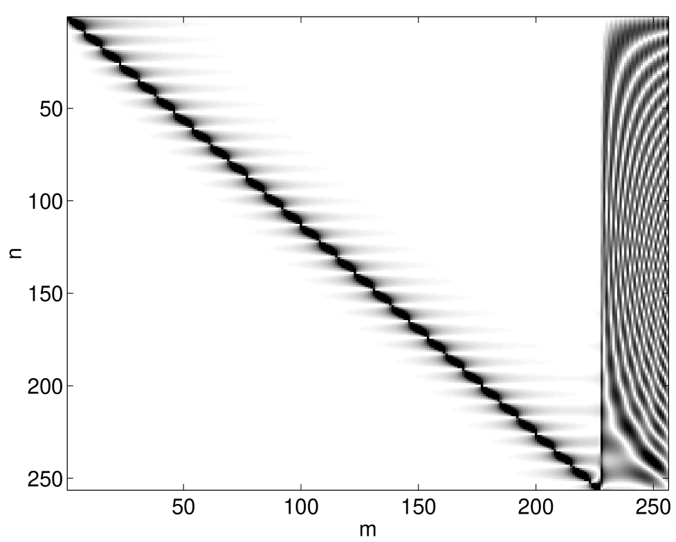
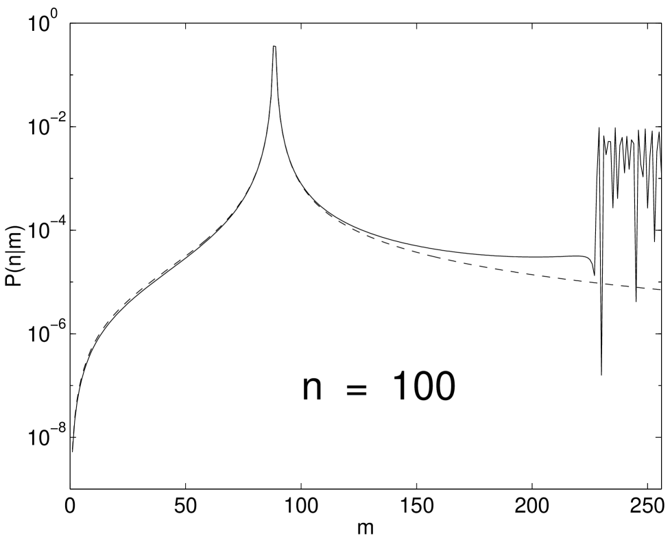
FIG. 2.: Upper subfigure: An image of the kernel $P(n|m)$ for $13\%$ expansion of the box (ie ${\mathsf{a}}/{\mathsf{a}}_{0}=1.13$). The kernel has been calculated numerically using Eq.(14) with finite truncation $N=256$. Lower subfigure: The profile of a representative row of $P(n|m)$. The dashed line is the $N=\infty$ analytical result using Eq.(12).

We can restore unitarity by making $V_{0}$ large but finite. In such case, a variation of the above calculation leads to the following picture: Consider the overlap of a reference level $n({\mathsf{a}})$ with the levels $m({\mathsf{a}}_{0})$. As in the case $V_{0}=\infty$ there is a probability $\eta$ which is located in the levels whose energies are $E_{m}\approx E_{n}$. But now the “lost” probability $(1-\eta)$ is located in the levels whose energies are $E_{m}\approx E_{n}+V_{0}$. Thus we have $\sum_{m}P(n|m)=1$ rather than $\sum_{m}P(n|m)=\eta$.

We consider again the case $V_{0}=\infty$. The normal derivative on the boundary is $\varphi_{n}({\mathsf{a}})=\sqrt{(2/{\mathsf{a}})}\ k_{n}$. Hence we can easily get the following result

$$\frac{1}{\hbar}{\mathbf{W}}_{nm}\ =\ \frac{-i}{k_{n}^{2}-k_{m}^{2}}\varphi_{n}({\mathsf{a}})\varphi_{m}({\mathsf{a}})\ =\ -i\frac{1}{{\mathsf{a}}}\frac{2nm}{n^{2}-m^{2}}$$ (13)

It is more convenient to use $\alpha=\ln({\mathsf{a}})$ for parameterization. Hence the equation that describes the parametric evolution is

$$\frac{da_{n}}{d\alpha}\ =\ -\sum_{m}\frac{2nm}{n^{2}-m^{2}}\ a_{m}$$ (14)

For any finite truncation $N<\infty$ this equation manifestly generates unitary parametric evolution. It is only for $N=\infty$ that it becomes equivalent to the non-unitary evolution of the 1D box. Again, one can wonder where the ‘lost’ probability is located if $N<\infty$. The answer is illustrated in Fig.2. We see that the ‘lost’ probability piles up at the edge of the (truncated) tail.

VI Matrix elements for chaotic cavity

It is possible to use semiclassical considerations [11] in order to determine the band profile of the matrix Eq.(8). The application to the cavity example has been introduced in [14], and numerically demonstrated in [17]. The accuracy of this semiclassical estimate is remarkable. Here we summarize the recipe. First one should generate a very long (ergodic) trajectory, and define for it the fluctuating quantity

$${\cal F}(t)=-\frac{\partial{\cal H}}{\partial x}=\sum_{\mbox{col}}2mv\ \cos(\theta_{\mbox{col}})\ D_{\mbox{col}}\ \delta(t-t_{\mbox{col}})$$ (15)

where $t_{\mbox{col}}$ is the time of a collision, $D_{\mbox{col}}$ stands for $D({\mathbf{s}})$ at the point of the collision, and $v\cos(\theta_{\mbox{col}})$ is the normal component of the particle’s velocity. Each delta spike (for soft walls it is actually a narrow rectangular spike) corresponds to one collision. Now one can calculate the correlation function $C(\tau)$ of the fluctuating quantity ${\cal F}(t)$, and its Fourier transform $\tilde{C}(\omega)$. The semiclassical estimate for the band profile is

$$\left\langle\left|\left(\frac{\partial{\cal H}}{\partial x}\right)_{nm}\right|^{2}\right\rangle\ \ \approx\ \ \frac{\Delta}{2\pi\hbar}\ \tilde{C}\left(\frac{E_{n}{-}E_{m}}{\hbar}\right)$$ (16)

Ref.[18] contains a systematic study of the function $\tilde{C}(\omega)$. For large $\omega$, meaning $\omega\gg 1/\tau_{\mbox{bl}}$, one can use

$$\tilde{C}(\omega)\ \approx\ 2m^{2}v^{3}\langle|\cos\theta|^{3}\rangle\frac{1}{{\mathsf{V}}}\oint[D({\mathbf{s}})]^{2}d{\mathbf{s}}$$ (17)

where the geometric factor is $\langle|\cos(\theta)|^{3}\rangle=1,4/3\pi,\cdots$ for $d=1,2,\cdots$. A lengthy calculation [14] reveals that Eq.(16) with (17) substituted, is an exact global result if we could assume that the cavity eigenfunctions look like ‘random waves’, and that different wavefunctions are uncorrelated. However, it turns out that to take this ‘random wave’ result as a global approximation is an over-simplification. For $\omega\ll 1/\tau_{\mbox{bl}}$, using the semiclassical recipe and assuming strongly chaotic cavity, one obtains

$$\tilde{C}(\omega)\ \approx\ \tilde{C}(\infty)\times(\tau_{\mbox{bl}}\omega)^{\gamma}$$ (18)

with $\gamma=4$ for dilations and translations, $\gamma=2$ for rotations, and $\gamma=0$ for normal deformations. We use the term ’special deformations’ [18] in order to distinguish those deformations that has the property $\tilde{C}(\omega)\rightarrow 0$ in the limit $\omega\rightarrow 0$. Any combination of dilations, translations and rotations is a special deformation. Around the bouncing frequency ($\omega\sim 1/\tau_{\mbox{bl}}$) the function $\tilde{C}(\omega)$ typically displays some non-universal (system and deformation specific) structure. This is true for any typical deformation, but for some deformations the non-universal features are more pronounced. If the cavity has bouncing ball modes, we may get also a modified (non-universal) behavior in the small frequency limit. For the purpose of general discussion it is convenient to assume that the interpolation between (18) and (17) is smooth, but in actual numerical calculation the actual $\tilde{C}(\omega)$ is computed (see below).

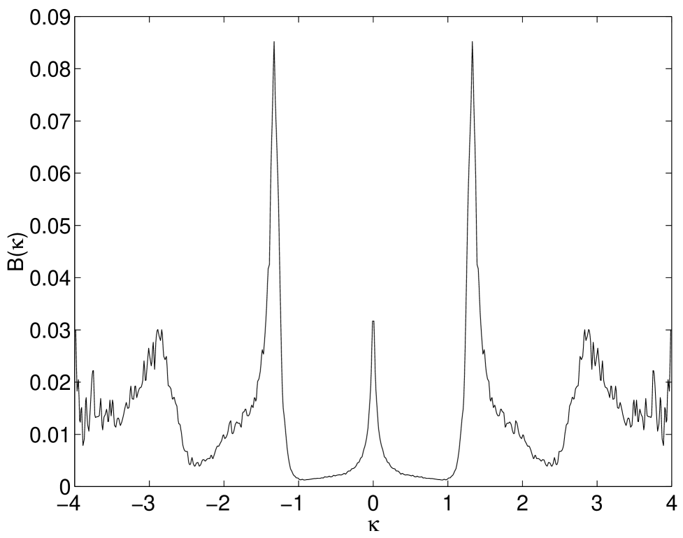
FIG. 3.: Band profiles for deformations of the quarter stadium as defined by Eq.(19). Upper plot: Rotation around the stadium center. Lower plot: Generic (non-special) deformation involving displacement of the curved edge. It is important to notice that for the special deformation we have $\tilde{C}(\omega)\rightarrow 0$ in the limit $\omega\rightarrow 0$.

As a numerical example we have picked the stadium billiard. We have found the eigenstates of a de-symmetrized (quarter) stadium as described in Ref.[17]. We have selected those eigenstates whose eigen-energies $k_{n}$ are in the vicinity of $k=400$. Our two representative deformations are: (a) rotation around the stadium center; and (b) generic (non-special) deformation involving the curved edge. In the latter case the curved edge of the quarter stadium ($0<s<\pi/2$) is pushed outwards with $D(s)=(\cos(s))^{2}$, while for the straight edges $D(s)=0$. (The corner $s=0$ is the $90^{\circ}$ intersection of the curved edge with the long straight edge). The respective band profiles are displayed in Fig.3. The band profile has been defined as

$$B(\kappa)\ =\ \frac{1}{4k^{2}}\ \left\langle\left|\oint\varphi_{n}({\mathbf{s}})\varphi_{m}({\mathbf{s}})\ D({\mathbf{s}})d{\mathbf{s}}\right|^{2}\right\rangle$$ (19)

where $\kappa=(k_{n}-k_{m})$ is the distance from the diagonal. Note that $B(\kappa)$ is just a scaled version of the semiclassical $\tilde{C}(\omega)$ as implied by Eq.(16) with (8). The remarkable agreement of $B(\kappa)$ with the semiclassical calculation has been demonstrated in [17, 18].

It is important to realize that in the hard wall limit (which is assumed here) the matrix $({\partial{\cal H}}/{\partial x})_{nm}$ is not a banded matrix. It would become banded if we were assuming soft walls. For soft walls $\tilde{C}(\omega)$ becomes vanishingly small for $\omega\gg v/\ell$. The bandwidth in energy units is $\Delta_{b}=\hbar v/\ell$, and in dimensionless units it is

$$b\ \ =\ \ \frac{\Delta_{b}}{\Delta}\ \ =\ \ \frac{{\mathsf{V}}}{\ell\ \lambda_{\mbox{B}}^{d{-}1}}$$ (20)

Unless stated otherwise we have $b=\infty$.

VII Parametric evolution - numerical results

The parametric evolution of $P(r)$ for rotation and for generic deformation of the stadium is illustrated by the images of Fig.4 and by the plots of Figs.5-6. The calculation of each $P(r)$ profile is carried out as follows: Given $\delta x$ we use the method which is described in [20] in order to calculate the matrix $P(n|m)$. Then we plot the elements of $P(n|m)$ versus $\kappa=(k_{n}(x)-k_{m}(0))$. In order to obtain the average profile the plot is smeared using standard procedure (see remark [21]). The transformation from $\kappa$ to $r=(n-m)$ is done using the relation (see remark [21]):

$$\kappa\ \ =\ \ \tilde{\Delta}\cdot r\ -\ \frac{1}{d}k\times\frac{\delta{\mathsf{V}}}{{\mathsf{V}}}$$ (21)

Above $\tilde{\Delta}$ is the mean level spacing of the $\{k_{n}\}$ spectrum, and $\delta{\mathsf{V}}$ is the volume change that is associated with the deformation (it is approximately proportional to $\delta x$). If the deformation is volume preserving (as in the case of rotation) then the second term equals zero. But for the generic deformation that we have picked in our second numerical example, the volume is not preserved, and the systematic ‘downwards’ shift of the levels should be taken into account.

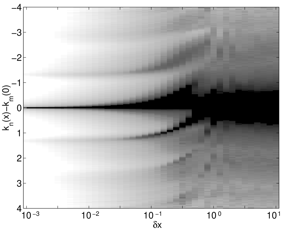
FIG. 4.: Each column is an image of $P(r)$ versus $\kappa$ for a different value of $\delta x$. There are 41 columns. The value $\delta x\sim 1$ corresponds roughly to $\lambda_{\mbox{B}}$ displacement of the boundary. The upper figure is for rotation, and the lower is for generic deformation. Note that the $r=0$ component is excluded from the image. Instead we have plotted over the image an $r=0$ line wherever this component contains more than $50\%$ of the probability. In the lower figure this line cannot be resolved from the developing core region.

Looking first in the case of rotation, we see clearly two parametric regimes: The standard perturbative regime ($\delta x<0.2$), and the non-universal regime ($\delta x>0.2$). Let us clarify this observation. We see that for $\delta x<0.2$ most of the probability is well concentrated in $r=0$. This implies that we can use standard perturbation theory in order to estimate the $r\neq 0$ probabilities. On the other hand for $\delta x>0.2$ the perturbative nature of $P(r)$ is destroyed. Now $P(r)$ becomes smoother, and eventually (for $\delta x>0.5$) there is a very good fitting with Lorentzian (see lower plot in Fig.5).

The qualitative explanation for the Lorentzian profile is as follows: For $\delta x>0.5$ the typical displacement of the walls is of the order of $\lambda_{\mbox{B}}$. Therefore the $|n(x)\rangle$ eigenstates become uncorrelated with the $|m(0)\rangle$ eigenstates. Consequently $P(r)$ becomes $\delta x$ independent. The Lorentzian profile agrees with the assumption of uncorrelated random waves as explained in Appendix A.

Let us look now in the case of generic deformation. Here we see clearly three parametric regimes: The standard perturbative regime ($\delta x<0.004$), the core-tail regime ($0.004<\delta x<0.2$), and the non-universal regime ($\delta x>0.2$). Let us clarify this observation. As in the case of rotation there is a standard perturbative regime ($\delta x<0.004$) where most of the probability is well concentrated in $r=0$. For larger deformation, namely for $\delta x>0.004$, standard perturbation theory is no longer applicable because the $n=m$ level is mixed non perturbatively with other (neighboring) levels. As a result $P(r)$ contains a non-perturbative ‘core’ component. However, for $0.004<\delta x<0.2$ we definitely do not get a Lorentzian. Rather the tails of $P(r)$ keep growing in the same way as in the standard perturbative regime.

In the case of the generic deformation, as in the case of rotation, we enter the non-universal regime, and eventually (for $\delta x>0.6$) we get a smooth Lorentzian-like distribution. However, the Lorentzian-like distribution is not identical with that of the rotation case. Also the similarity to proper Lorentzian is far from being satisfactory. (see lower plot in Fig.6). This means that the random-wave picture of Appendix A is an oversimplification.

In the following sections we are going to summarize the theoretical considerations [8] that explain the observed parametric scenario. In particular we are going to illuminate the way in which non-perturbative features emerge; to clarify the crossover to the non-universal regime; and to explain the specific nature of the non-universal distribution.

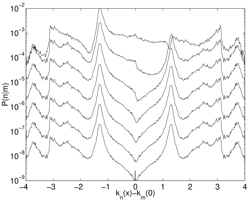
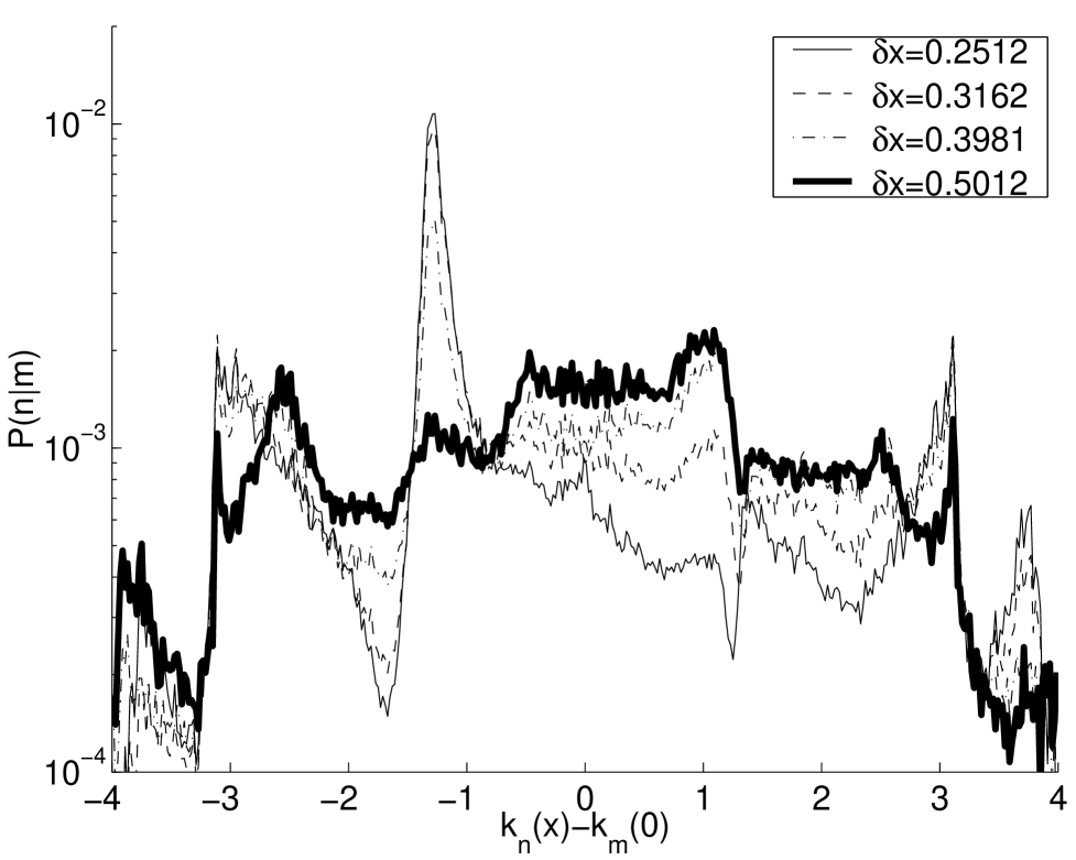
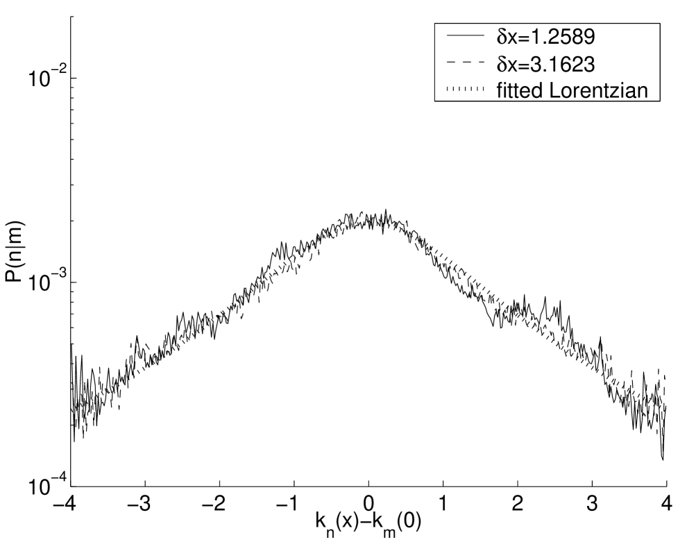
FIG. 5.: Representative plots of $P(r)$ for the case of rotation. The upper subfigure is for $0.0010\leq\delta x\leq 0.2512$. The $r=0$ component is excluded. In the lower subfigure the fitted Lorentzian is indistinguishable from the actual profile.

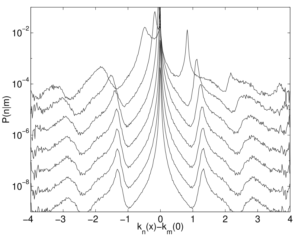
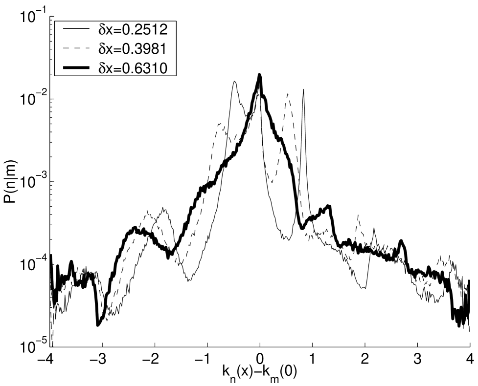
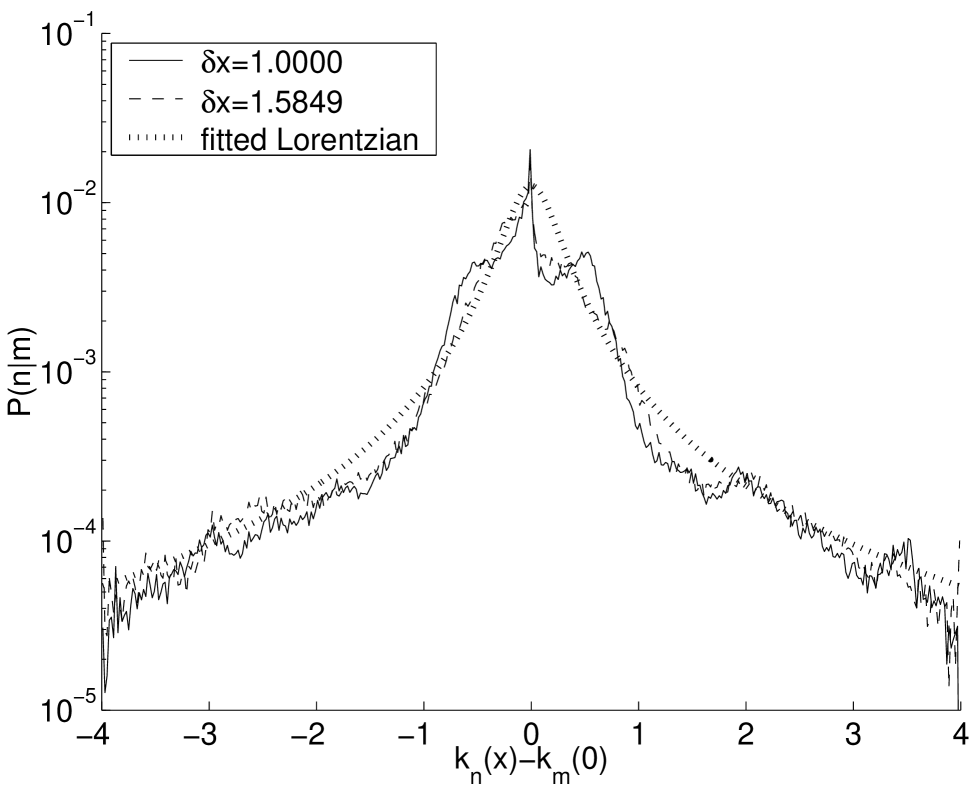
FIG. 6.: Representative plots of $P(r)$ for the case of generic deformation. The upper subfigure is for $0.0010\leq\delta x\leq 0.2512$. In the lower subfigure a fitted Lorentzian is overlayed for the purpose of comparison.

VIII The standard perturbative regime

Standard perturbation theory gives the following first order expression for the LDOS

$$P(n|m)\ \ \approx\ \ \delta_{nm}\ +\ \delta x^{2}\frac{|({\partial{\cal H}}/{\partial x})_{nm}|^{2}}{(E_{n}-E_{m})^{2}}$$ (22)

This expression is most straightforwardly obtained by inspecting Eqs.(5) and (6). We can define the (total) transition probability as

$$p(\delta x)\ \ =\ \ \sum_{r\neq 0}P(r)$$ (23)

Using Eq.(22) combined with (16) we get the following estimate:

$$p(\delta x)\ \ \approx\ \ \delta x^{2}\times\frac{1}{\hbar^{2}}\int_{|\omega|>\frac{\Delta}{\hbar}}\frac{d\omega}{2\pi}\ \frac{\tilde{C}(\omega)}{\omega^{2}}$$ (24)

Standard perturbation theory is applicable as long as $p(\delta x)\ll 1$. This can be converted into an equivalent inequality $\delta x\ll\delta x_{c}^{\mbox{qm}}$. By this definition $\delta x_{c}^{\mbox{qm}}$ is the parametric deformation which is needed in order to mix the initial level $m$ with other levels $n\neq m$.

If we use Eq.(24) for a special deformation, then we have $\gamma>1$, and consequently the integral is not sensitive to the exclusion of the $|r|<\Delta$ region. As a result we have $\delta x_{c}^{\mbox{qm}}\propto\hbar$. Using Eq.(18) with (17) we get

$$\delta x_{c}^{\mbox{qm}}|_{\mbox{special}}\ \ =\ \ \left(\ell_{\mbox{bl}}\frac{1}{{\mathsf{V}}}\oint[D({\mathbf{s}})]^{2}d{\mathbf{s}}\right)^{-\mbox{$\frac{1}{2}$}}\times\lambda_{\mbox{B}}$$ (25)

In case of generic deformation Eq.(25) is not valid because the value of the integral in (24) is predominantly determined by the $\omega\sim\Delta/\hbar$ lower cutoff rather than by an effective $\omega\sim 1/\tau_{\mbox{bl}}$ lower cutoff. As a result one obtains

$$\delta x_{c}^{\mbox{qm}}|_{\mbox{generic}}\ \ =\ \ \left(\ell_{\mbox{H}}\frac{1}{{\mathsf{V}}}\oint[D({\mathbf{s}})]^{2}d{\mathbf{s}}\right)^{-\mbox{$\frac{1}{2}$}}\times\lambda_{\mbox{B}}$$ (26)

where $\ell_{\mbox{H}}=vt_{\mbox{H}}$ is the length which is associated with the Heisenberg time $t_{\mbox{H}}=2\pi\hbar/\Delta$.

It is illuminating to use the convention $D({\mathbf{s}})\sim 1$, such that $\delta x$ measures the typical displacement of a wall element. With this convention we get from Eqs.(25)-(26) the following:

$$\delta x_{c}^{\mbox{qm}} |_{\mbox{special \hskip 9.95845pt}}\ \ \approx\ \ \lambda_{\mbox{B}}$$ (27)

$$\delta x_{c}^{\mbox{qm}} |_{\mbox{generic \hskip 9.95845pt}}\ \ =\ \ \left(\frac{\lambda_{\mbox{B}}^{d{-}1}}{{\mathsf{A}}_{\mbox{eff}}}\right)^{\mbox{$\frac{1}{2}$}}\times\lambda_{\mbox{B}}$$ (28)

$$\delta x_{c}^{\mbox{qm}} |_{\mbox{diffractive}}\ \ \sim\ \ \lambda_{\mbox{B}}$$ (29)

In the generic case the effective area of the deformed boundary ${\mathsf{A}}_{\mbox{eff}}$ may be smaller than the total area ${\mathsf{A}}$ of the boundary. The effective area ${\mathsf{A}}_{\mbox{eff}}$ can be formally defined by comparing Eq.(28) with Eq.(26). Eq.(29) has been added for sake of completeness of our presentation. It correspond to the diffractive limit ${\mathsf{A}}_{\mbox{eff}}\rightarrow\lambda_{\mbox{B}}^{d{-}1}$. Note that this limit is beyond the scope of the present study. Thus in the generic case, the wall displacement needed to mix levels is much smaller than $\lambda_{\mbox{B}}$. In the generic case $\delta x_{c}^{\mbox{qm}}\propto\hbar^{(d{+}1)/2}$ rather than $\delta x_{c}^{\mbox{qm}}\propto\hbar$. What happens with perturbation theory beyond $\delta x_{c}^{\mbox{qm}}$? This is the subject of the next section.

IX The core-tail regime

For $\delta x>\delta x_{c}^{\mbox{qm}}$ standard perturbation theory diverges due to the non-perturbative mixing of neighboring levels on small scale: Once $\delta x$ becomes of the order of $\delta x_{c}^{\mbox{qm}}$ several levels are mixed, and as $\delta x$ becomes larger, more levels are being mixed non-perturbatively. Consequently it is natural to distinguish between core and tail regions [13, 14, 15]. Most of the spreading probability is contained within the core region, which implies a natural extension of first-order perturbation theory (FOPT): The first step is to transform Eq.(5) into a new basis where transitions within the core are eliminated; The second step is to use FOPT (in the new basis) in order to analyze the core-to-tail transitions. Details of this procedure, which is in the spirit of degenerate perturbation theory, were discussed in [14]. The most important (and non-trivial) consequence of this procedure is the observation that mixing on small scales does not affect the transitions on large-scales. Therefore we have in the tail region $P(n|m)\propto\delta x^{2}$ rather than $P(n|m)\propto\delta x$. The validity of this observation has been numerically illustrated in [15].

Following the above reasoning we define the tail region as consists of those levels whose ‘occupation’ can be calculated using perturbation theory, while the core is the non-perturbative component in the vicinity of $r=0$. Assuming that only one scale characterize the core width, one arrives at the following practical approximation:

$$P_{\mbox{prt}}(r)=\frac{\Delta}{2\pi\hbar}\ \tilde{C}\left(\frac{E_{n}{-}E_{m}}{\hbar}\right)\ \frac{\delta x^{2}}{(\Gamma(\delta x))^{2}+(E_{n}{-}E_{m})^{2}}$$ (30)

It is implicit in this definition that $(E_{n}{-}E_{m})$ should be regarded as a function of $r=(n-m)$. The parameter $\Gamma(\delta x)$ is determined (for a given $\delta x$) such that $P_{\mbox{prt}}(r)$ has a unit normalization. One may say that $\Gamma(\delta x)$ regularizes the behavior around $r=0$. For generic deformation we get

$$\Gamma(\delta x)\ \equiv\ b_{0}\Delta\ \approx\ \left(\frac{\delta x}{\delta x_{c}^{\mbox{qm}}}\right)^{2}\times\Delta$$ (31)

The core is defined as the region $|r|<b_{0}$, and the outer ($|r|>b_{0}$) regions are the tails. For $\delta x\ll\delta x_{c}^{\mbox{qm}}$ we get $b_{0}\ll 1$ and the core-tail structure Eq.(30) becomes equivalent to the standard perturbative result Eq.(22). It should be clear that the core-tail structure is a generalization of Wigner’s Lorentzian. It is indeed a Lorentzian in the special case of a ‘flat’ band profile.

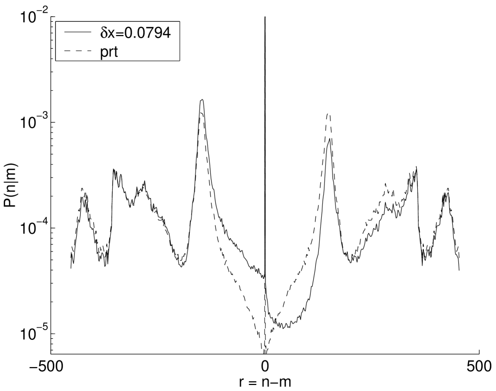
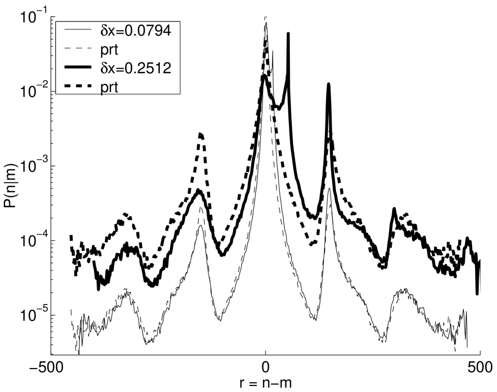
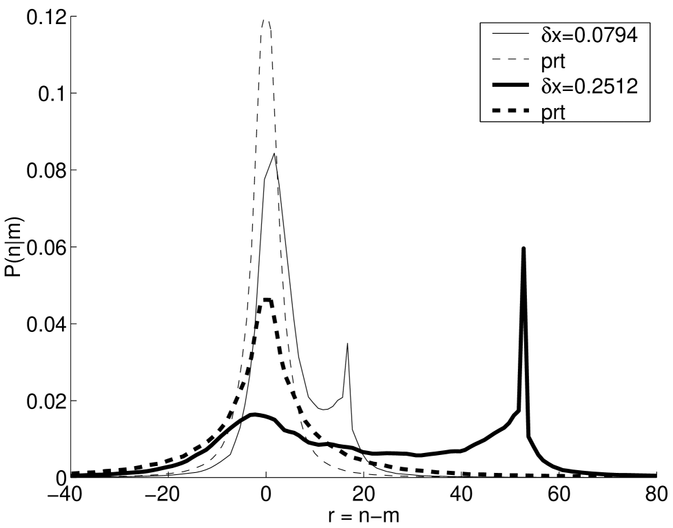
FIG. 7.: Comparison between the perturbative calculation $P_{\mbox{prt}}(r)$ and the actual $P(r)$. The upper subfigure is for the rotation and the lower subfigures are for the generic deformation. The lower subfigure gives a zoom over the the ‘birth’ of the non-perturbative semiclassical saturation profile.

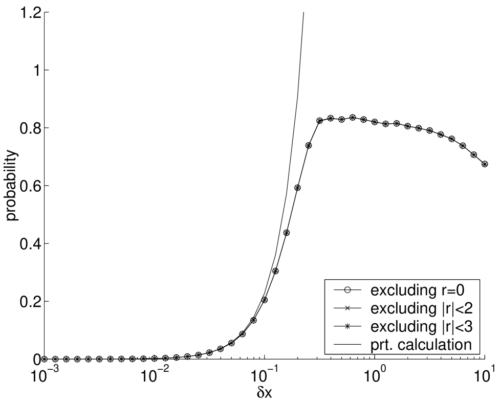
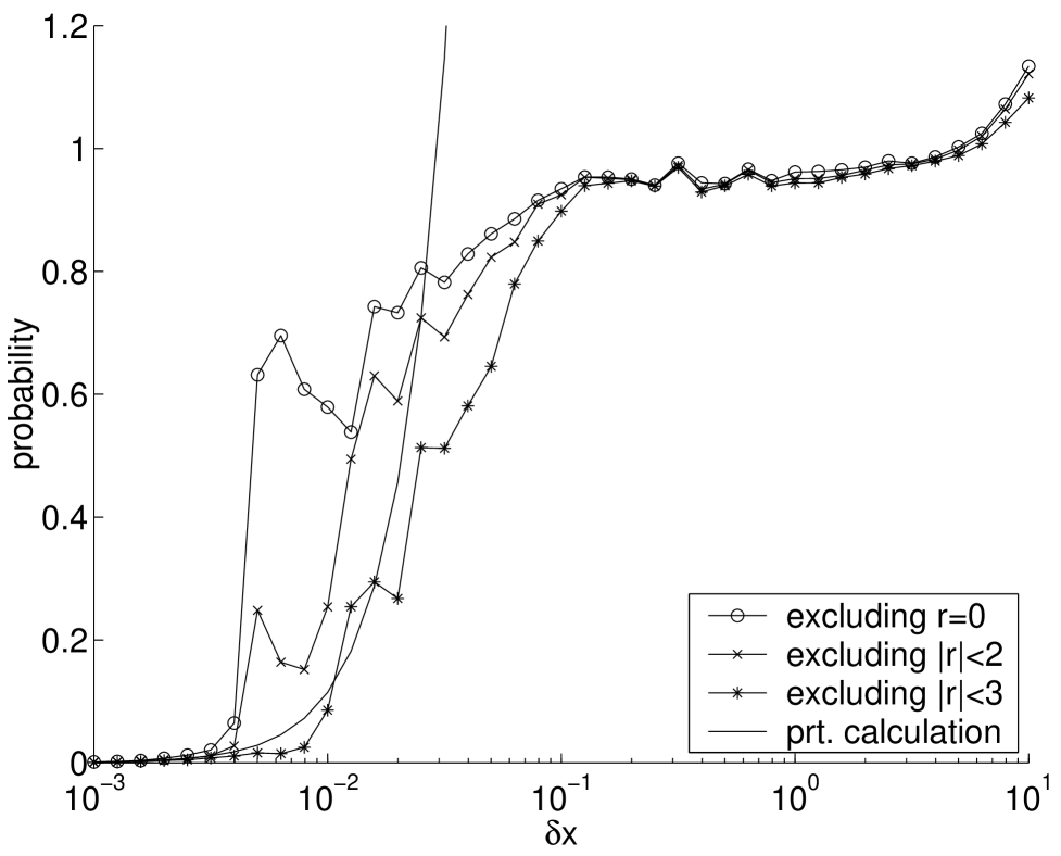
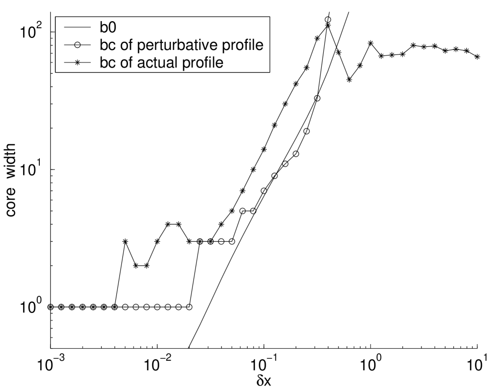
FIG. 8.: The upper and the middle subfigures are $p(\delta x)$ for the rotation and for the generic deformation respectively. The lower subfigure is the perturbative calculation of the core width $b_{0}$ for the generic deformation. Also displayed is the calculated $b_{c}$ for $P_{\mbox{prt}}(r)$, and the actual $b_{c}$ for $P(r)$.

We turn now to analyze our numerical results. We have verified (see eg Fig.7) that for $\delta x<0.2$ we have good agreement with perturbation theory irrespective of whether we have a core component (which is the case for the generic deformation) or not (which is the case for the rotation). As we come closer to $\delta x\sim 0.2$ the agreement becomes worse, and for $\delta x>0.3$ we have a total collapse of perturbation theory. In Fig.8 we display the total transition probability $p(\delta x)$ as a function of $\delta x$. This plot should be used in order to numerically determine the value of $\delta x_{c}^{\mbox{qm}}$, say as the value where $p(\delta x)=1/2$.

Fig.8 also displays comparison with the corresponding perturbative calculation (using Eq.(23) with(30)). The agreement (for $\delta x<\delta x_{c}^{\mbox{qm}}$) in case of the rotation is remarkable. For larger values of $\delta x$ one observes a linear drop of the total probability due to the non-unitary nature of the evolution. (This drop is clearly linear in a linear-linear scale which is not displayed). The eventual rise of the total transition probability (beyond $1$) in case of the generic deformation, reflects numerical errors in the determination of the small $\kappa$ overlaps. See [20] for further details.

The lower subfigure in Fig.8 displays the calculated core width $b_{0}$ for the generic deformation. Recall that $b_{0}$ is determined, given $\delta x$, such that $P_{\mbox{prt}}(r)$ of Eq.(30) is normalized. Also calculated is the width $b_{c}$ of the region that contains $50\%$ of the probability. The width $b_{c}$ is calculated for both $P_{\mbox{prt}}(r)$ and $P(r)$. Note that $b_{c}=1$ in the standard perturbative regime. The determination of $\delta x_{c}^{\mbox{qm}}$ for the generic deformation becomes more convenient by using this plot. Also the crossover (at $\delta x_{\mbox{NU}}\sim 0.2$) to the non-universal regime is most pronounced.

X The non-universal regime

The validity of Eq.(30) as a global approximation relies on the assumption that the core is characterized only by one scale (which is $b_{0}$). But this assumption ceases to be true if $\delta x$ is large enough. We have explained in Ref.[8] that the width of the core defines a ‘window’ through which we can view the ‘landscape’ of the semiclassical analysis. As $\delta x$ becomes larger, this ‘window’ becomes wider, and eventually some of semiclassical structure is exposed. This is marked by the non-universal parametric scale $\delta x_{\mbox{NU}}$. For $\delta x$ larger than $\delta x_{\mbox{NU}}$, the non-universal structure of the core is exposed.

What is the semiclassical structure of the LDOS? Time-domain semiclassical considerations (See Eq.(10) of [8] and related discussion there) imply that the non-universal structure of the core is

$$P(n-m)\ \ \approx\ \ \frac{1}{\pi}\ \frac{\delta E_{\mbox{SC}}}{\delta E_{\mbox{SC}}^{2}+(E_{n}{-}E_{m})^{2}}$$ (32)

with $\delta E_{\mbox{SC}}=\hbar/\tau_{\mbox{col}}$. The definition of the collision rate $1/\tau_{\mbox{col}}$ is similar to that of $1/\tau_{\mbox{bl}}$. The former is the collision rate with the deformed area ${\mathsf{A}}_{\mbox{dfr}}$, and therefore it may be smaller than $1/\tau_{\mbox{bl}}$, because $\tau_{\mbox{bl}}$ is related to the total area ${\mathsf{A}}$.

If, by mistake, we identified $\tau_{\mbox{col}}$ with $\tau_{\mbox{bl}}$, then we would get the random wave result which is derived in Appendix A. This would be an over simplification. If it were true, it would imply that for $\delta x>\delta x_{\mbox{NU}}$ we should have got the same Lorentzian-distribution in both cases (the rotation and the generic deformation). What we see, as a matter of fact, is that for the rotation (Fig.5) we have a reasonably good agreement with Lorentzian whose width is $\delta k_{\mbox{SC}}=1.5$, whereas for the generic deformation (Fig.6) there is rough agreement with Lorentzian whose width is $\delta k_{\mbox{SC}}=0.26$. The smaller width in the latter case clearly reflects having larger $\tau_{\mbox{col}}$. For the generic deformation we also have pronounced non-Lorentzian features. Actually the global fitting to Lorentzian is quite bad. Our understanding is that these features are due to the bouncing-ball trapping: It leads to non-exponential decay of the time-dependent survival probability (see [8] for definition of the latter term), and hence to the observed non Lorentzian features of the spreading profile.

We turn now to explain how $\delta x_{\mbox{NU}}$ is determined. By definition it is the deformation which is required in order to expose features of the semiclassical landscape. These features start to be exposed once $\Gamma(\delta x)\sim\delta E_{\mbox{SC}}$ which should be converted into an equivalent expression $\delta x\sim\delta x_{\mbox{NU}}$. Thus we get

$$\delta x_{\mbox{NU}}\ \ =\ \ \left(\frac{{\mathsf{A}}_{\mbox{dfr}}}{{\mathsf{A}}_{\mbox{eff}}}\right)^{\mbox{$\frac{1}{2}$}}\times\lambda_{\mbox{B}}\ \ \sim\ \ \lambda_{\mbox{B}}$$ (33)

Here ${\mathsf{A}}_{\mbox{dfr}}$ is the geometric area of the deformation (in the sense of scattering cross-section), while ${\mathsf{A}}_{\mbox{eff}}$ is the effective area of the deformation. The definition of the latter is implied by comparing Eq.(28) with Eq.(26). By rescaling $D({\mathbf{s}})\mapsto\alpha D({\mathbf{s}})$ and $\delta x\mapsto\delta x/\alpha$, we can make ${\mathsf{A}}_{\mbox{eff}}={\mathsf{A}}_{\mbox{dfr}}$ by convention. For special deformations $\delta x_{\mbox{NU}}$ coincides with $\delta x_{c}^{\mbox{qm}}$ implying that we get into the non-universal regime as soon as we have a breakdown of standard perturbation theory.

Our theoretical consideration so far do not imply a total collapse of perturbation theory. We may have in principle a co-existence of non-universal core component and perturbative tails. Actually we see such co-existence in the lower subfigures of Fig.7, mainly for $\delta x=0.2512$. The right peak around $\kappa=0$ is clearly non-perturbative, while the rest of the profile is in reasonable (though not very good) agreement with the perturbative calculation. We are going to explain in the next section that the total collapse of perturbation theory for $\delta x>0.3$ is actually not related at all to the appearance of non-universal features in the core structure. It is only circumstantial that in the hard wall limit this collapse happens as soon as we enter the non-universal regime.

XI The collapse of perturbation theory

A good starting for the following discussion is to consider the classical approximation for $P(r)$. Namely, in Eq.(1) one approximates $\rho_{n}(Q,P)$ and $\rho_{m}(Q,P)$ by microcanonical distributions. A phase-space illustration of the energy surfaces which support $\rho_{n}(Q,P)$ and $\rho_{m}(Q,P)$ can be found in Fig.1 of Ref.[8]. The classical $P(n|m)$ equals to the overlap of these surfaces.

If we were dealing with a generic system we could introduce a linearized version of the Hamiltonian ${\cal H}(Q,P;x)={\cal H}_{0}(Q,P)+\delta x{\cal F}(Q,P;\delta x{=}0)$, where ${\cal F}(Q,P;x)={\partial{\cal H}}/{\partial x}$. By definition this linearization is a good approximation provided $\delta x\ll\delta x_{c}^{\mbox{cl}}$, where $\delta x_{c}^{\mbox{cl}}$ is the classical correlation scale of ${\cal F}(Q,P;x)$ with respect to $x$. In the classical linear regime the classical $P(r)$ has the scaling property $P(r)=1/\delta x\hat{P}(r/\delta x)$.

An equivalent definition of $\delta x_{c}^{\mbox{cl}}$ in the quantum-mechanical case is obtained by looking on the $x$ dependence of the matrix elements of ${\cal F}(Q,P;x)$ in some fixed basis. Again we define $\delta x_{c}^{\mbox{cl}}$ as the respective correlation scale. It is quite clear that for cavity with soft walls we have

$$\delta x_{c}^{\mbox{cl}}\ \ =\ \ \ell\ \ \ \ \mbox{[soft walls]}$$ (34)

where $\ell=E/f$ has been defined as the penetration distance upon collision. From purely classical point of view the hard wall limit $\ell\rightarrow 0$ is a non-linear limit. But this is not true quantum-mechanically. Here we have

$$\delta x_{c}^{\mbox{cl}}\ \ \sim\ \ \lambda_{\mbox{B}}\ \ \ \ \mbox{[hard walls]}$$ (35)

for $\ell<\lambda_{\mbox{B}}$. The terminology ‘classical correlation scale’ while referring to $\delta x_{c}^{\mbox{cl}}$ becomes misleading here, but we shall keep using it anyway.

The theory of the core-tail structure [14] is valid only in the linear regime $\delta x\ll\delta x_{c}^{\mbox{cl}}$. Let us assume for a moment soft walls. We can ask: Is $\delta x\ll\delta x_{c}^{\mbox{cl}}$ a sufficient condition for having a core-tail structure? The answer is definitely not. Perturbation theory has a final collapse once the core width $b_{0}(\delta x)$ becomes of the order of the band width $b$. This defines a parametric scale $\delta x_{\mbox{prt}}$. For $\delta x>\delta x_{\mbox{prt}}$ the LDOS becomes purely non-perturbative. In Wigner’s theory of random banded matrices this corresponds to the crossover from Lorentzian to semicircle line shape.

However, in the limit of hard walls the above mechanism of collapse becomes irrelevant because the band width is infinite ($b=\infty$). On the other hand we still have to satisfy the inequality $\delta x\ll\delta x_{c}^{\mbox{cl}}$. Thus, for $\delta x>\lambda_{\mbox{B}}$ we expect a total collapse of perturbation theory, as indeed observed in the numerical study.

A Overlap of uncorrelated random waves

It is possible to estimate the overlap $|\langle n|m\rangle|^{2}$ if we assume that $|n\rangle$ and $|m\rangle$ are uncorrelated random-superpositions of plane-waves: A random-superpositions of plane-waves is characterized by the correlation function

$$\langle\psi_{\mbox{R}}({\mathbf{x}}_{1})\psi_{\mbox{R}}({\mathbf{x}}_{2})\rangle\ =\ \frac{1}{{\mathsf{V}}}\ \mbox{Cos}(k|{\mathbf{x}}_{2}-{\mathbf{x}}_{1}|)$$ (A1)

where $\mbox{Cos}(kr)\equiv\langle\exp(i{\mathbf{k}}\cdot{\mathbf{r}})\rangle_{\Omega}$ is a generalized Bessel function (for further details see Appendix D of [14]). Assuming that the wavefunction of $|n\rangle$ is uncorrelated with the wavefunction of $|m\rangle$ one obtains

$$\langle|\langle n|m\rangle|^{2}\rangle\ =\ \left(\frac{1}{{\mathsf{V}}}\right)^{2}\times\hskip 113.81102pt$$ (A2)

$$\int\!\int\mbox{Cos}(k_{n}|{\mathbf{x}}_{2}{-}{\mathbf{x}}_{1}|)\ \mbox{Cos}(k_{m}|{\mathbf{x}}_{2}{-}{\mathbf{x}}_{1}|)\ \ d{\mathbf{x}}_{1}d{\mathbf{x}}_{2}$$ (A3)

The integration is over the whole volume of the cavity. Using the definition of the Cos function we can cast this expression into the form $\langle|\langle n|m\rangle|^{2}\rangle=\left\langle f({\mathbf{q}})\right\rangle_{q}$ where the average is over the difference ${\mathbf{q}}=({\mathbf{k}}_{2}-{\mathbf{k}}_{1})$, with all possible orientations for $|{\mathbf{k}}_{1}|=k_{m}$ and for $|{\mathbf{k}}_{2}|=k_{n}$. The function $f({\mathbf{q}})$ is defined as follows:

$$f({\mathbf{q}})\ =\ \left|\int\mbox{e}^{i{\mathbf{q}}{\cdot}{\mathbf{x}}}d{\mathbf{x}}\right|^{2}$$ (A4)

The function $f({\mathbf{q}})$ depends mainly on $q=|{\mathbf{q}}|$. We can obtain an estimate for $f(q)$ by considering a spherical cavity $|{\mathbf{x}}|<R$ with the same volume. Using spherical coordinates it is straightforward to obtain the following:

$$f(q)\ \approx\ \left({\cal FT}\left[\frac{1}{d{-}1}(R^{2}-x^{2})^{(d{-}1)/2}\right]\right)^{2}$$ (A5)

above ${\cal FT}$ is a Fourier transform from $x$ to $q$. For $q\ll 1/R$ we have simply $f(q)=({\mathsf{V}})^{2}$. For $q\gg 1/R$ we have $f(q)=({\mathsf{V}})^{2}/(Rq)^{d{+}1}$. This is because of the singularity at $x=\pm R$. The average over $q$ can be done using again spherical coordinate. We have $q\approx((\Delta k)^{2}+2k^{2}(1-\cos\theta))^{\mbox{1/2}}$, where $\Delta k=|k_{n}-k_{m}|$, and we can transform the $d\theta$ integration into $dq$ integration:

$$\left\langle f({\mathbf{q}})\right\rangle_{q}\ \ =\ \ \frac{\Omega_{d{-}2}}{\Omega_{d{-}1}}\times\hskip 113.81102pt$$ (A6)

$$\int\ \frac{qdq}{k^{2}}\left(\frac{\sqrt{(q^{2}-(\Delta k)^{2})((2k)^{2}-q^{2})}}{2k^{2}}\right)^{d{-}3}f(q)$$ (A7)

where $\Omega_{d}$ is the solid angle in $d$ dimensions. There is no point in trying to carry an exact integration. Rather, it is important to observe that a practical approximation for the overlap is:

$$\langle|\langle n|m\rangle|^{2}\rangle\ \approx\ \left(\frac{1}{kR}\right)^{d{-}1}\frac{1}{1+(R{\cdot}(k_{n}{-}k_{m}))^{2}}$$ (A8)

In the latter expression we have neglected the $d$-dependent normalization prefactor. It is a ‘practical’ approximation since it gives the correct behavior for both small and large values of $\Delta k$. The interpolation around $\Delta k\sim 1/R$ cannot be trusted.

Acknowledgments:

This work was funded by ITAMP and the National Science Foundation.

REFERENCES

- [1] The classical approximation for works well for ergodic eigenstates. As explained later in the text we actually consider the averaged profile. Namely, is regarded as a function of , and it is averaged over the reference state . With this procedure the effect of the minority of non-ergodic eigenstates can be neglected in the classical limit.
- [2] The two parametric scales of Wigner’s RMT model correspond to and of Table 1. Consequently there are three parametric regimes in Wigner’s theory. These are the standard perturbative regime (), the Lorentzian regime (), and the semi-circle regime (). As an artifact of this RMT model, there actually exists a forth regime (Anderson strong localization regime) that in the present context does not have a semiclassical analog.
- [3] As explained in [8] the generic hierarchy is . This hierarchy is realized in the classical limit (small ) where we have soft walls (see section II). The hard wall limit is non-generic, and these four parametric scales coincide. In the present paper we assume hard walls unless stated otherwise.
- [4] G. Casati, B.V. Chirikov, I. Guarneri, F.M. Izrailev, Phys. Rev. E 48, R1613 (1993); Phys. Lett. A 223, 430 (1996).
- [5] V.V. Flambaum, A.A. Gribakina, G.F. Griobakin and M.G. Kozlov, Phys. Rev. A 50 267 (1994).
- [6] G. Casati, B.V. Chirikov, I. Guarneri and F.M. Izrailev, Physics Lett. A 223, 430 (1996). F. Borgonovi, I. Guarneri and F.M. Izrailev Phys. Rev. E 57, 5291 (1998).
- [7] E. Heller in Chaos and quantum Physics, Proc. Session LII of the Les-Houches Summer School, Edited by A. Voros and M-J Giannoni (Amsterdam: North Holland 1990).
- [8] D. Cohen and E.J. Heller, Phys. Rev. Lett. 84, 2841 (2000).
- [9] Atom-photon interactions: basic processes and applications, C. Cohen-Tannoudji, J. Dupont-Roc and G. Grynberg (New York: J. Wiley 1992).
- [10] E. Wigner, Ann. Math 62, 548 (1955); 65, 203 (1957).
- [11] M. Feingold and A. Peres, Phys. Rev. A 34 591, (1986). M. Feingold, D. Leitner, M. Wilkinson, Phys. Rev. Lett. 66, 986 (1991). M. Wilkinson, M. Feingold, D. Leitner, J. Phys. A 24, 175 (1991). M. Feingold, A. Gioletta, F. M. Izrailev, L. Molinari, Phys. Rev. Lett. 70, 2936 (1993).
- [12] D. Cohen, Phys. Rev. Lett. 82, 4951 (1999).
- [13] D. Cohen, in Proceedings of the International School of Physics ‘Enrico Fermi’ Course CXLIII “New Directions in Quantum Chaos”, Edited by G. Casati, I. Guarneri and U. Smilansky, IOS Press, Amsterdam, 2000.
- [14] D. Cohen, Annals of Physics 283, 175 (2000).
- [15] D. Cohen and T. Kottos, nlin.CD/0001026, Phys. Rev. E (2001, in press).
- [16] M. V. Berry and M. Wilkinson, Proc. R. Soc. London A 392, 15 (1984).
- [17] A. Barnett, D. Cohen, and E.J. Heller, Phys. Rev. Lett. 85, 1412 (2000).
- [18] A. Barnett, D. Cohen, and E.J. Heller, nlin.CD/0006041, J. Phys. A (2001, in press).
- [19] E. Vergini and M. Saraceno, Phys. Rev. E, 52, 2204 (1995). E. Vergini, Ph. D. thesis, Universidad de Buenos Aires, 1995.
- [20] A. Barnett, PhD thesis (Harvard, Sept. 2000).
- [21] In order to find the average profile we divide the axis into small bins. We find the average value in each bin. In order to get we re-sample the average profile. The distance between the sampling points is equal to the mean level spacing. We are not interested in features on scale of the mean level spacing. Therefore the transformation from the continuous variable to the integer variable should not be considered as problematic.