Upper Bound on the Products of
Particle Interactions in Cellular Automata

Abstract

Particle-like objects are observed to propagate and interact in many spatially extended dynamical systems. For one of the simplest classes of such systems, one-dimensional cellular automata, we establish a rigorous upper bound on the number of distinct products that these interactions can generate. The upper bound is controlled by the structural complexity of the interacting particles—a quantity which is defined here and which measures the amount of spatio-temporal information that a particle stores. Along the way we establish a number of properties of domains and particles that follow from the computational mechanics analysis of cellular automata; thereby elucidating why that approach is of general utility. The upper bound is tested against several relatively complex domain-particle cellular automata and found to be tight.

Keywords: Cellular automata, Particles, Gliders, Domains, Particle interactions, Domain transducer

PACS: 45.70.Qj, 05.45, 05.65+b

Contents

toc

I Introduction

Persistent, localized, propagating structures—particles—have long been observed and constructed in cellular automata (CAs) [1, 2, 3, 4, 5, 6, 7, 8, 9, 10, 11, 12, 13, 14, 15, 16, 17, 18, 19, 20, 21, 22]. A review of the literature suggests that particles are widely felt to be some of the more interesting phenomena displayed by those systems [23]. They are analogous to the “defects” or “coherent structures” of pattern formation processes in condensed matter physics [4, 5, 8, 9, 16, 18]. In fact, in cellular automata used to model pattern formation processes, the particles model defects and vice versa [24, 25, 26, 27]. A different analogy to condensed matter physics (specifically, hydrodynamics [28]) gives them the name “solitons” [8, 9]. They are also known as gliders, glider-like objects, or spaceships particularly, but not exclusively, in the context of the Game of Life two-dimensional CA [2, 29]. The name “particle”, while inspired by an analogy to field theory in physics, is used here merely for the sake of uniform terminology and neutrality of associations.

CA particles, like their physical counterparts, interact via collision, and these interactions are well known to play a crucial role in the dynamics of their underlying cellular automaton. The construction of computational devices in CAs, for instance, is almost always accomplished through engineering the proper interactions among particles [1, 12, 13, 33, 34, 35, 36, 37, 38, 39, 40, 41]. Indeed, it was even at one time conjectured by Wolfram [42] that the presence of particles in a CA was tantamount to its being computation-universal. It is therefore of considerable interest to know what interactions a CA’s particles may have. Acquiring that knowledge is significantly simplified if we can place a bound on the number of different interactions between any pair of particles. The first successful attempt to do so was an expression given in [9] for particles interacting on a completely uniform, quiescent background. It has been appreciated for some time, however, that many CAs display patterned or textured backgrounds—sometimes called “domains”. Here we substantially generalize the original formula to accommodate a large class of domains and prove the generalization using elementary automata and number theory.

The outline of the paper is as follows. First, we fix basic notation relating to cellular automata, regular languages, and finite-state transducers. We then define domains, in particular periodic domains, and prove some basic results about them. We next define particles as a particular kind of interface between domains, and define interactions between particles. After establishing some auxiliary number-theoretic results, we prove the upper bound formula that generalizes the main theorem of [9] to arbitrary periodic domains. Result in hand, we show how it applies to the analysis of several CAs encountered in applications, and how it simplifies the analysis of their particle dynamics. We close with a summary of the results and a list of open questions. An appendix gives the details of the proof of an auxiliary result on domains.

The present work is motivated by and bears on several larger issues. Of particular relevance is the notion of an “object” or “coherent structure” that spontaneously emerges in the space-time behavior of a process [43, 44]. The particles analyzed here are arguably one of the simplest kinds of such emergent structures. Despite this interest, we do not define “particle” from first principles. Like our predecessors we take the existence of particles as a given and assume we know how to recognize them in the space-time behavior. Nonetheless, the results and their proofs do elucidate some of the component concepts that we feel will be useful in a theory of emergent structures in spatial processes.

II Cellular Automata, Formal Languages, and Transducers

A cellular automaton (CA) is a discrete dynamical system consisting of a regular lattice of identical cells. At each time step $t$, each of these cells is in one of a number $k$ of states $\Sigma$. The state of cell $i$ at time $t$ is denoted $s^{i}_{t}\in\Sigma\equiv\{0,1,\ldots,k-1\}$. The global state ${\bf s}_{t}$ of a one-dimensional CA at time $t$ is the configuration of the entire lattice; i.e., ${\bf s}_{t}=(s^{0}_{t},s^{1}_{t},\ldots,s^{N-1}_{t})\in\Sigma^{N}$, where $N$ is the lattice size. One often sees CA phenomenology studied where $\Sigma=\{0,1\}$ and with periodic boundary conditions: $s^{N+i}_{t}=s^{i}_{t}$. The main results reported below do not depend on these restrictions, however.

At each next time step $t+1$, the cells in the lattice update their states simultaneously according to a local update rule $\phi$. This update rule $\phi$ takes as input the current local neighborhood configuration $\eta^{i}_{t}=(s^{i-r}_{t},\ldots,s^{i}_{t},\ldots,s^{i+r}_{t})$ of cell $i$ and returns the next state $s^{i}_{t+1}$; $r$ is the CA’s radius. Thus, the CA equations of motion are given by

$$s^{i}_{t+1}=\phi(\eta^{i}_{t})~{}.$$ (1)

The global update rule $\Phi:\Sigma^{N}\rightarrow\Sigma^{N}$ applies $\phi$ in parallel (simultaneously) to all cells in the CA lattice; i.e.,

$${\bf s}_{t+1} = \Phi({\bf s}_{t})$$ (2)

$$= \left(\phi(\eta^{0}_{t}),\phi(\eta^{1}_{t}),\ldots\phi(\eta^{N-1}_{t})\right)~{}.$$ (3)

Binary $(k=2)$ local state, $r=1$ CAs are referred to as elementary CAs (ECAs) [47].

An ensemble operator $\boldsymbol{\Phi}$ can be defined [20, 48] that operates on sets of lattice configurations $\Omega_{t}=\{{\bf s}_{t}\}$:

$$\Omega_{t+1}=\boldsymbol{\Phi}\Omega_{t}~{},$$ (4)

such that

$$\Omega_{t+1}=\{{\bf s}_{t+1}:{\bf s}_{t+1}=\Phi({\bf s}_{t}),~{}{\bf s}_{t}\in\Omega_{t}\}~{}.$$ (5)

It is often informative to describe CA configurations as one or another type of formal language. A formal language $\mathcal{L}$ over the alphabet $\Sigma$ is a subset of $\Sigma^{*}$—the set of all possible words, or strings, made up of symbols from $\Sigma$. A regular language is a formal language whose words can be generated or recognized by a device with finite memory; sometimes called a finite automaton. Regular languages are the simplest class of formal languages in a hierarchy (the Chomsky hierarchy) of language classes of increasing complexity [49].

A deterministic finite automaton (DFA) $M$ is defined as a 5-tuple:

$$M=\{Q,\Sigma,\delta,q_{0},F\}~{},$$ (6)

where $Q$ is a finite set of states, $\Sigma$ is an alphabet, $q_{0}\in Q$ is the initial state, $F\subseteq Q$ is a set of final states, and $\delta:Q\times\Sigma\rightarrow Q$ is a transition function: $\delta(q,a)=q^{\prime}$, where $q,q^{\prime}\in Q$ and $a\in\Sigma$.

A DFA can be used to read, or scan, words $w=w_{1}\ldots w_{L}$ over the alphabet $\Sigma$. Starting in the initial state $q_{0}$, the DFA reads the first symbol $w_{1}$ of the word $w$. It then makes a transition to another state $q^{\prime}=\delta(q_{0},w_{1})$. The DFA then reads the next symbol $w_{2}$ and makes a transition to $q^{\prime\prime}=\delta(q^{\prime},w_{2})$, and so on until all symbols in $w$ have been read or until an undefined transition is encountered. If, after reading $w$, the DFA ends in a final state $q\in F$, $M$ accepts $w$; otherwise $M$ rejects it.

A regular language $\mathcal{L}$ is a formal language for which there exists a DFA that accepts all words in $\mathcal{L}$ and rejects all words not in $\mathcal{L}$. If there is one such DFA, there are generally many of them, but there is a unique minimal DFA for ${\mathcal{L}}$, which we write $M({\mathcal{L}})$. Similarly, for every DFA $M$ there is a corresponding regular language ${\mathcal{L}}(M)$ consisting of all and only the words that are accepted by $M$. The regular process languages are a subset of the regular languages: those containing all subwords of words in the language. All states of the corresponding DFA—the process graph—are both initial and accepting states [20].

Finally, a finite-state transducer (FST) is a finite automaton with two kinds of symbol associated with each transition: inputs and outputs. Formally, an FST $R$ is defined as a 7-tuple:

$$R=\{Q,\Sigma_{in},\Sigma_{out},\delta,\lambda,q_{0},F\}~{},$$ (7)

where $Q,\delta,q_{0},$ and $F$ are as in a DFA, $\Sigma_{in}$ is the input alphabet, $\Sigma_{out}$ is the output alphabet, and $\lambda:Q\times\Sigma_{in}\rightarrow\Sigma_{out}$ is the observation function: $\lambda(q,a)=b$ where $q\in Q$, $a\in\Sigma_{in}$, and $b\in\Sigma_{out}$. An FST effectively implements a mapping $f_{R}$ from one language over $\Sigma_{in}$ to another language over $\Sigma_{out}$. In other words, it reads a word $w\in\Sigma_{in}^{*}$ and transforms it to another word $w^{\prime}\in\Sigma_{out}^{*}$ by mapping each symbol $w_{i}\in\Sigma_{in}$ to a symbol $w_{i}^{\prime}\in\Sigma_{out}$ such that $w_{i}^{\prime}=\lambda(q,w_{i})$, where $q\in Q$ is the current state of $R$ when reading $w_{i}$.

In formal language theory, languages and automata play the role of sets and transducers the role of functions.

III Domains

We are now ready to review the computational mechanics analysis of emergent structures in CAs [20, 50].

A regular domain $\Lambda$ of a CA $\Phi$ is a process language, representing a set of spatial lattice configurations, with the following properties:

1. Temporal invariance (or periodicity): $\Lambda$ is mapped onto itself by the CA dynamic; i.e., $\boldsymbol{\Phi}^{p}\Lambda=\Lambda$ for some finite $p$. (Recall that $\mathbf{\Phi}$ takes sets of lattice configurations into sets of configurations and that a formal language, such as $\Lambda$, is a set of configurations.)

2. Spatial homogeneity: The process graph of each temporal iterate of $\Lambda$ is strongly connected. That is, there is a path between every pair of states in $M(\Phi^{l}\Lambda)$ for all $l$. (Recall that $M({\mathcal{L}})$ is the minimal DFA which recognizes the language $\mathcal{L}$.)

The set of all domains of a CA $\Phi$ is denoted $\boldsymbol{\Lambda}=\{\Lambda^{0},\Lambda^{1},\dots,\Lambda^{m-1}\}$, where $m=|\boldsymbol{\Lambda}|$.

According to the first property—temporal invariance or periodicity—a particular domain $\Lambda^{i}$ consists of $p$ temporal phases for some $p\geq 1$; i.e., $\Lambda^{i}=\{\Lambda_{0}^{i},\Lambda_{1}^{i},\ldots,\Lambda_{p-1}^{i}\}$, such that $\boldsymbol{\Phi}^{l}\Lambda_{j}^{i}=\Lambda_{(j+l)\bmod p}^{i}$. Here $p$ is the temporal periodicity of the domain $\Lambda^{i}$; which we denote by $T(\Lambda^{i})$.

Each of the temporal phases $\Lambda_{j}^{i}$ of a domain $\Lambda^{i}$ is represented by a process graph $M(\Lambda^{i}_{j})$ which, according to the second property (spatial homogeneity), is strongly connected. Each of these process graphs consists of a finite number of states. We denote the ${k}^{\mathrm{t}h}$ state of the ${j}^{\mathrm{t}h}$ phase of $\Lambda^{i}$ by $\Lambda_{j,k}^{i}$, intentionally suppressing the $M(\cdot)$ notation for conciseness. We write the number of states in a given phase as $S(\Lambda_{j}^{i})$.

The process graphs of all temporal phases $\Lambda^{i}_{j}$ of all domains $\Lambda^{i}$ can be connected together and transformed into a finite-state transducer, called the domain transducer, that reads in a spatial configuration and outputs various kinds of information about the sites. (The construction is given in, for example, [51].) Variations on this transducer can do useful recognition tasks. For example, all transitions that were in domain $\Lambda^{i}_{j}$’s process graph are assigned output symbol $D$, indicating that the input symbol being read is “participating” in a domain. All other transitions in the transducer indicate deviations from the sites being in a domain. They can be assigned a unique output (“wall”) symbol $w\in\{W^{i}_{j}\}$ that labels the kind of domain violation that has occurred. The resulting domain transducer can now be used to filter CA lattice configuration, mapping all domain regularities to $D$ and mapping all domain violations to output symbols $w$ that indicate domain walls of various kinds.

We say that a phase of a domain is (spatially) periodic when the process graph consists of a periodic chain of states, with a single transition between successive states in the chain. That is, as one moves from state to state, an exactly periodic sequence of states is encountered and an exactly periodic sequence of symbols from $\Sigma$ is encountered on the transitions. The spatial periodicity of a periodic phase is simply $S(\Lambda^{i})$. We say that a domain is periodic when all its phases are periodic. Almost all of our attention in the sequel will be confined to periodic domains, for the following reason. It turns out that for such domains all of the spatial periodicities $S(\Lambda_{j}^{i})$ at each temporal phase are equal. Thus, we can speak of the spatial periodicity $S(\Lambda^{i})$ of a periodic domain $\Lambda^{i}$. This property, in turn, is central to our proof of the upper bound on the number of particle interaction products.

Lemma 1

If a domain $\Lambda^{i}$ has a periodic phase, then the domain is periodic, and the spatial periodicities $S(\Lambda^{i}_{j})$ of all its phases $\Lambda^{i}_{j},j=0,\ldots,p-1,$ are equal.

Proof. See the Appendix. $\Box$

Thus, the number of states in the process graph representing a particular temporal phase $\Lambda^{i}_{j}$ is the same for all $j\in\{1,\ldots,T(\Lambda^{i})\}$, and it is, in fact, $S(\Lambda^{i})$.

Finally, there is a larger class of cyclic domains whose process graphs consist of a periodic chain of states: as one moves from state to state an exactly periodic sequence of states is seen. Note that this class includes more than periodic domains, which are obviously cyclic. It includes domains in which between two successive states in the chain there are multiple transitions over $\Sigma$. (See [51] for a CA exhibiting two such cyclic domains.) Based on our experience we conjecture that Prop. 1 also holds for cyclic domains. If this is so, most of the following results, and in particular the upper bound theorem, would hold for this large class.

Conjecture 1

For any cyclic domain $\Lambda^{i}$, the spatial periodicities $S(\Lambda^{i}_{j})$ of all its phases $\Lambda^{i}_{j},j=0,\ldots,p-1,$ are equal.

IV Particles

When domain violations form a spatially localized (finite width), temporally periodic boundary between two adjacent domains, they are called particles.

Definition 1

A particle $\alpha$ is a set $\{\alpha^{0},\alpha^{1},\ldots,\alpha^{p-1}\}$ of finite-width words $\alpha^{j}$ over $\Sigma^{*}$, called wedges, such that

$${\boldsymbol{\Phi}}(\Lambda\alpha^{i}\Lambda^{\prime})=\Lambda\alpha^{(i+1)\bmod p}\Lambda^{\prime}~{},$$ (8)

for some finite $p$ and $\Lambda$ and $\Lambda^{\prime}\in\boldsymbol{\Lambda}$.

Since a particle is a bounded structure, it does not have a spatial periodicity. In the following, the “periodicity of a particle” therefore refers to temporal periodicity.

Since these particles are temporally periodic, we view the appearance of wedge $\alpha^{j}$ as the particle being in it’s $j$th phase. The $k$th symbol in the wedge’s word is denoted $\alpha^{j}_{k}$. The state in which the domain transducer finds itself after reading the $k$th symbol $\alpha^{j}_{k}$ in the wedge $\alpha^{j}$ is denoted $q(\alpha^{j}_{k})$.

We now introduce an important but subtle distinction. The particle period $p$ referred to above—the surface periodicity—is associated with the repetition over time of the wedge words as observed in the raw space-time behavior ${\boldsymbol{s}}_{0},{\boldsymbol{s}}_{1},{\boldsymbol{s}}_{2},\ldots$. It turns out, as will become clear, that particles have an internal periodicity that may be some multiple of the surface periodicity $p$. The internal periodicity—the one of actual interest here—though, is the periodicity seen by the various phases of the bordering domains.

Definition 2

A particle $\alpha$’s intrinsic periodicity $P(\alpha)$ is the periodicity of the set of transducer-state sequences generated when reading a particle’s wedges. For wedge $\alpha^{j}=\alpha^{j}_{0}\ldots\alpha^{j}_{n}$ the state sequence $q(\alpha^{j}_{0})\ldots q(\alpha^{j}_{n})$ is generated in the transducer. We denote this state sequence by $q(\alpha^{j})$. $P(\alpha)$, then, is the number of iterations over which the sequence $q(\alpha^{j})$ reappears.

Remark 1. $P(\alpha)$ is an integer multiple of $\alpha$’s apparent periodicity.

Remark 2. A simple illustration of the need for intrinsic, as opposed to merely surface, periodicity is provided by the $\gamma$ particles of ECA 54. See Fig. 4(b) and the accompanying text in Sec. VII A.

After one period $P(\alpha)$, a particle $\alpha$ will have moved a number $d_{\alpha}$ of sites in the CA lattice. This shift $d_{\alpha}$ in space after one period is called the particle’s displacement. $d_{\alpha}$ is negative for displacements to the left and positive for displacements to the right. From the particle’s periodicity $P(\alpha)$ and displacement $d_{\alpha}$, its average velocity is simply $v_{\alpha}=d_{\alpha}/P(\alpha)$.

Note that the above remarks hold whether we are looking at the wedges or at the transducer-state labeled wedges: one obtains the same velocity.

The set of all particles $\alpha,\beta,\ldots$ of a CA $\Phi$ is denoted by $\bf P$.

Remark 3. Here we defined temporally periodic particles. There are particles in CAs, such as in ECA 18, which are temporally aperiodic. In this case, one replaces the periodicity condition Eq. (8) by one using the ensemble operator; viz.,

$$\boldsymbol{\Phi}^{p}(\Lambda\alpha\Lambda^{\prime})=\Lambda\alpha\Lambda^{\prime}~{}.$$ (9)

A Structural Complexity of a Particle

The preceding definitions and discussion suggest that one can think of particles as having an internal clock or, in the more general case that includes aperiodic particles, an internal state, much as the solitary-wave solutions of continuum envelope equations have internal states [28]. One can ask about how much information a particle stores in its states. This is the amount of information that a particle transports across space and time and brings to interactions. These considerations lead one to a natural measure of the amount of structural complexity associated with individual particles.

Definition 3

The structural complexity $C(\alpha)$ of a particle $\alpha$ is defined to be

$$C(\alpha)=-\sum_{j=0}^{p-1}{\rm Pr}(q(\alpha^{j}))\log_{2}{{\rm Pr}(q(\alpha^{j}))}~{},$$ (10)

where $p$ is $\alpha$’s period and ${\rm Pr}(q(\alpha^{j}))$ is the probability of $\alpha$ being in phase $\alpha^{j}$ with the state-sequence $q(\alpha^{j})$.

Remark 1. For the straightforward case of periodic particles, in which the wedges and so their associated state sequences are equally probable, we have

$$C(\alpha)=\log_{2}{P(\alpha)}~{}.$$ (11)

Remark 2. The information available to be processed in particle interactions is upper-bounded by the sum of the individual particle complexities, since this sum assumes independence of the particles. As we will see shortly, the relative information—that information in one particle, conditioned on the other’s phase (via the constraints imposed by the mediating domain) and suitably averaged—determines the information available for processing by interactions.

B Domain Transducer View of Particle Phases

A particle is bounded on either side by two patches of domain. (They could be patches of the same or different domains.) Consider what happens to the domain transducer as it scans across the part of the lattice containing the bounding domains ($\Lambda^{i}$ and $\Lambda^{i^{\prime}}$) and the particle ($\alpha$). It begins by cycling through the states of the process graph of a phase ($j$) of the first bounding domain ($\Lambda^{i}$). It then encounters a symbol that does not belong to the language of that domain phase, and this then causes a transition out of that process graph. Each successive symbol of the particle wedge leads to additional transitions in the transducer. Finally, the transducer reaches cells at the beginning of the other bounding domain ($\Lambda^{i^{\prime}}$), whereupon it begins to follow the process graph of $\Lambda^{i^{\prime}}_{j^{\prime}}$ at some appropriate phase $j^{\prime}$. In this way, a particle wedge $\alpha^{j}$ corresponds to a sequence $q(\alpha^{j})$ of transducer states.

More formally, the transducer maps a particle wedge $\alpha^{j}$, bordered by $\Lambda^{i}_{j}$ and $\Lambda^{i^{\prime}}_{j^{\prime}}$, to an ordered $n-$tuple ($n=|\alpha^{j}|+2$) of states

$$Q(\alpha^{j}) = \left<q(\Lambda^{i}_{j,k}),q(\alpha^{j}),q(\Lambda^{i^{\prime}}_{j^{\prime},k^{\prime}})\right>~{},$$ (12)

where $q(\Lambda^{i}_{j,k})$ is the transducer state reach on reading symbol $\Lambda^{i}_{j,k}$. Since the transducer-state sequence is determined by the bounding domain phases and the actual wedge $\alpha^{j}$, it follows that the mapping from particle wedges to state sequences is 1-1. If two particle wedges correspond to the same sequence of states, then they are the same phase of the same particle, and vice versa.

This representation of particle phases will prove very handy below.

V Interactions

In many CAs, when two or more particles collide they create another set of particles or mutually annihilate. Such particle interactions are denoted $\alpha+\beta\rightarrow\gamma$, for example. This means that the collision of an $\alpha$ particle on the left and a $\beta$ particle on the right leads to the creation of a $\gamma$ particle. Particle annihilation is denoted $\alpha+\beta\rightarrow\emptyset$. For completeness we note that there are also unstable walls that can spontaneously decay into particles. This is denoted $\alpha\rightarrow\beta+\gamma$, for example.

Often, the actual product of a particle interaction depends on the phases $\alpha^{j}$ and $\beta^{k}$ in which the interacting particles are at the time of collision. In such a case, there can be more than one interaction product for a particular collision: e.g., both $\alpha+\beta\rightarrow\gamma$ and $\alpha+\beta\rightarrow\emptyset$ can be observed.

The set of a CA’s possible particle interactions is denoted $\bf I$. The complete information about a CA’s domains $\boldsymbol{\Lambda}$, particles $\bf P$, and particle interactions $\bf I$ can be summarized in a particle catalog. The catalog forms a high-level description of the CA’s dynamics. It is high-level in the sense of capturing the dynamics of emergent structures. The latter are objects on a more abstract level than the original equations of motion and raw (uninterpreted) spatial configurations of site values.

VI Bounding the Number of Interaction Products

Restricting ourselves to particle interactions with just two colliding particles—$\alpha$ and $\beta$, say—we now give an upper bound on the number $n_{\alpha,\beta}$ of possible interaction products from a collision between them. (See Fig. 1 for the interaction geometry.) In terms of the quantities just defined, the upper bound, stated as Thm. 22 below, is:

$$n_{\alpha,\beta}\leq\frac{P(\alpha)P(\beta)\Delta v}{T(\Lambda^{i})S(\Lambda^{i})}~{},$$ (13)

where $\Delta v=v_{\alpha}-v_{\beta}>0$ and $\Lambda^{i}$ is the domain in between the two particles before they collide. Note that if $\Delta v=0$, then $n_{\alpha,\beta}=0$ trivially.

For simplicity, in the rest of the development we assume that $\Delta v=v_{\alpha}-v_{\beta}\geq 0$. This simply means that particle $\alpha$ lies to the left of $\beta$ and they move closer to each other over time, as in Fig. 1.

FIG. 1.: Interactions between an $\alpha$ and a $\beta$ particle with domain $\Lambda$ lying between.

This section proves that Eq. (13) is indeed a proper upper bound. The next section gives a number of examples, of both simple and complicated CAs, that show the bound is and is not attained. These highlight an important distinction between the number of possible interactions (i.e., what can enter the interaction region) and the number of unique interaction products (i.e., what actually leaves the interaction region).

To establish the bound, we collect several intermediate facts. The first three lemmas come from elementary number theory. Recall that the least common multiple ${\rm lcm}(a,b)$ of two integers $a$ and $b$ is the smallest number $c$ that is a multiple of both $a$ and $b$. Similarly, the greatest common divisor $\gcd(a,b)$ of two integers $a$ and $b$ is the largest number $c$ that divides both $a$ and $b$.

Lemma 2

$\gcd(ca,cb)=c\;\gcd(a,b),\;c>0$.

Proof. See Thm. 2.7 in [52]. $\Box$

Lemma 3

$\gcd(a,b)\;{\rm lcm}(a,b)=ab$.

Proof. See Thm. 2.8 in [52]. $\Box$

Lemma 4

${\rm lcm}(ca,cb)=c\;{\rm lcm}(a,b),\;c>0$.

Proof. Using Lemmas 2 and 3, it follows that

$${\rm lcm}(ca,cb) = \frac{cacb}{\gcd(ca,cb)}$$ (14)

$$= c\frac{ab}{\gcd(a,b)}$$ (15)

$$= c\;{\rm lcm}(a,b)~{}.$$ (16)

$\Box$

Now we are ready to begin building an analysis of particles and particle interactions.

Lemma 5

The intrinsic periodicity $P(\alpha)$ of a particle $\alpha$ is a multiple of the temporal periodicity $T(\Lambda^{i})$ of either domain $\Lambda^{i}$ for which $\alpha$ is a boundary. That is,

$$P(\alpha)=m_{\alpha i}T(\Lambda^{i})~{},$$ (17)

for some positive integer $m_{\alpha i}$ that depends on $\alpha$ and $\Lambda^{i}$.

Proof. At any given time, a configuration containing the particle $\alpha$ consists of a patch of the domain $\Lambda^{i}$, a wedge belonging to $\alpha$, and then a patch of $\Lambda^{i^{\prime}}$, in that order from left to right. (Or right to left, if that is the chosen scan direction.) Fix the phase of $\alpha$ to be whatever we like — $\alpha^{l}$, say. This determines the phases of $\Lambda^{i}$, for the following reason. Recall that, being a phase of a particle, $\alpha^{l}$ corresponds to a unique sequence $Q(\alpha^{l})$ of transitions in the domain transducer. That sequence starts in a particular domain-phase state $\Lambda^{i}_{j,k}$ and ends in another domain-phase state $\Lambda^{i^{\prime}}_{j^{\prime},k^{\prime}}$. So, the particle phase $\alpha^{l}$ occurs only at those times when $\Lambda^{i}$ is in its $j^{\rm th}$ phase. Thus, the temporal periodicity of $\alpha$ must be an integer multiple of the temporal periodicity of $\Lambda^{i}$. By symmetry, the same is also true for the domain $\Lambda^{{i}^{\prime}}$ to the right of the wedge. $\Box$

Corollary 1

Given that the domain $\Lambda^{i}$ is in phase $\Lambda^{i}_{j}$ at some time step, a particle $\alpha$ forming a boundary of $\Lambda^{i}$ can only be in a fraction $1/T(\Lambda^{i})$ of its $P(\alpha)$ phases at that time.

Proof. This follows directly from Lemma 5.

Remark. Here is the first part of the promised restriction on the information in multiple particles. Consider two particles $\alpha$ and $\beta$, separated by a domain $\Lambda^{0}$. Naively, we expect $\alpha$ to contain $\log_{2}{P(\alpha)}$ bits of information and $\beta$, $\log_{2}{P(\beta)}$ bits. Given the phase of $\alpha$, however, the phase of $\Lambda^{0}$ is fixed, and therefore the number of possible phases for $\beta$ is reduced by a factor of $1/T(\Lambda^{0})$. Thus the number of bits of information in the $\alpha$-$\beta$ pair is at most

$$\log_{2}{P(\alpha)}+\log_{2}{P(\beta)}-\log_{2}{T(\Lambda^{0})}=\log_{2}{\frac{P(\alpha)P(\beta)}{T(\Lambda^{0})}}~{}.$$ (18)

The argument works equally well starting from $\beta$.

Lemma 6

For any two particles $\alpha$ and $\beta$, the quantity ${\rm lcm}(P(\alpha),P(\beta))\Delta v$ is a non-negative integer.

Proof. We know that the quantity is non-negative, since the least common multiple always is and $\Delta v$ is so by construction. It remains to show that their product is an integer. Let ${k_{\alpha}}={{\rm lcm}(P(\alpha),P(\beta))/P(\alpha)}$ and ${k_{\beta}}={{\rm lcm}(P(\alpha),P(\beta))/P(\beta)}$; these are integers. Then

$$\Delta v \equiv \frac{d_{\alpha}}{P(\alpha)}-\frac{d_{\beta}}{P(\beta)}$$

$$= \frac{{k_{\alpha}}{d_{\alpha}}-{k_{\beta}}{d_{\beta}}}{{\rm lcm}(P(\alpha),P(\beta))}~{}.$$

When multiplied by ${\rm lcm}(P(\alpha),P(\beta))$ this is just ${k_{\alpha}}{d_{\alpha}}-{k_{\beta}}{d_{\beta}}$, which is an integer. $\Box$

Lemma 7

When the distance $d$ between two approaching particles $\alpha$ and $\beta$, in phases $\alpha^{j}$ and $\beta^{j^{\prime}}$, respectively, is increased by ${\rm lcm}(P(\alpha),P(\beta))\Delta v$ sites, the original configuration—distance $d$ and phases $\alpha^{j}$ and $\beta^{j^{\prime}}$—recurs after ${\rm lcm}(P(\alpha),P(\beta))$ time steps.

Proof. From the definition of ${\rm lcm}(a,b)$ it follows directly that ${\rm lcm}(P(\alpha),P(\beta))$ is a multiple of $P(\alpha)$. Thus,

$$\alpha^{(j+{\rm lcm}(P(\alpha),P(\beta)))\bmod P(\alpha)}=\alpha^{j}~{},$$ (19)

and the $\alpha$ particle has returned to its original phase. Exactly parallel reasoning holds for the $\beta$ particle. So, after ${\rm lcm}(P(\alpha),P(\beta))$ time steps both $\alpha$ and $\beta$ are in the same phases $\alpha^{j}$ and $\beta^{j^{\prime}}$ again. Furthermore, in the same amount of time the distance between the two particles has decreased by ${\rm lcm}(p_{\alpha},p_{\beta})\Delta v$, which is the amount by which the original distance $d$ was increased. (By Lemma 6, that distance is an integer, and so we can meaningfully increase the particles’ separation by this amount.) Thus, after ${\rm lcm}(P(\alpha),P(\beta))$ time steps the original configuration is restored. $\Box$

Lemma 8

If $\Lambda^{i}$ is the domain lying between two particles $\alpha$ and $\beta$, then the ratio

$$r=\frac{{\rm lcm}(P(\alpha),P(\beta))\Delta v}{S(\Lambda^{i})}$$ (20)

is an integer.

Proof. Suppose, without loss of generality, that the particles begin in phases $\alpha^{0}$ and $\beta^{0}$, at some substantial distance from each other. We know from the previous lemma that after a time ${\rm lcm}(P(\alpha),P(\beta))$ they will have returned to those phases and narrowed the distance between each other by ${\rm lcm}(P(\alpha),P(\beta))\Delta v$ cells. What the lemma asserts is that this displacement is some integer multiple of the spatial periodicity of the intervening domain $\Lambda^{i}$. Call the final distance between the particles $d$. Note that the following does not depend on what $d$ happens to be.

Each phase of each particle corresponds to a particular sequence of transducer states—those associated with reading the particle’s wedge for that phase. Reading this wedge from left to right (say), we know that $Q(\alpha^{0})$ must end in some phase-state of the domain $\Lambda^{i}$; call it $\Lambda^{i}_{0,0}$. Similarly, $Q(\beta^{0})$ must begin with a phase-state of $\Lambda^{i}$, but, since every part of the intervening domain is in the same phase, this must be a state of the same phase $\Lambda^{i}_{0}$; call it $\Lambda^{i}_{0,k}$. In particular, consistency requires that $k$ be the distance between the particles modulo $S(\Lambda^{i})$. But this is true both in the final configuration, when the separation between the particles is $d$, and in the initial configuration, when it is $d+{\rm lcm}(P(\alpha),P(\beta))\Delta v$. Therefore

$$d+{\rm lcm}(P(\alpha),P(\beta))\Delta v = d\pmod{S(\Lambda^{i})}$$

$${\rm lcm}(P(\alpha),P(\beta))\Delta v = 0\pmod{S(\Lambda^{i})}~{}.$$

Thus, ${\rm lcm}(P(\alpha),P(\beta))\Delta v$ is an integer multiple of the spatial period $S(\Lambda^{i})$ of the intervening domain $\Lambda^{i}$. $\Box$

Remark. It is possible that ${\rm lcm}(P(\alpha),P(\beta))\Delta v=0$, but this does not affect the subsequent argument. Note that if this is the case, then, since the least common multiple of the periods is at least $1$, we have $\Delta v=0$. This, in turn, implies that the particles do not, in fact, collide and interact, and so the number of interaction products is simply zero. The formula gives the proper result in this case.

The next result follows easily from Lemmas 2 and 5.

Lemma 9

If $\Lambda^{i}$ is the domain lying between particles $\alpha$ and $\beta$, then

$$\gcd(P(\alpha),P(\beta))=T(\Lambda^{i})\gcd(m_{\alpha i},m_{\beta i})~{}.$$ (21)

Proof. We apply Lemma 4:

$$\gcd(P(\alpha),P(\beta)) = \gcd(m_{\alpha i}T(\Lambda^{i}),m_{\beta i}T(\Lambda^{i})$$

$$= T(\Lambda^{i})\gcd(m_{\alpha i},m_{\beta i}).$$

$\Box$

With the above lemmas the following theorem can be proved, establishing an upper bound on the number of possible particle interaction products.

Theorem 1

The number $n_{\alpha,\beta}$ of products of an interaction between two approaching particles $\alpha$ and $\beta$ with a domain $\Lambda^{i}$ lying between is at most

$$n_{\alpha,\beta}\leq\frac{P(\alpha)P(\beta)\Delta v}{T(\Lambda^{i})S(\Lambda^{i})}~{}.$$ (22)

Proof. First, we show that this quantity is an integer. We use Lemma 3 to note that

$$\frac{P(\alpha)P(\beta)\Delta v}{T(\Lambda^{i})S(\Lambda^{i})}=\frac{\gcd(P(\alpha),P(\beta)){\rm lcm}(P(\alpha),P(\beta))\Delta v}{T(\Lambda^{i})S(\Lambda^{i})}~{},$$ (23)

and then Lemma 8 to find that

$$\frac{P(\alpha)P(\beta)\Delta v}{T(\Lambda^{i})S(\Lambda^{i})}=\frac{\gcd(P(\alpha),P(\beta))r}{T(\Lambda^{i})}~{},$$ (24)

and finally Lemma 21 to show that

$$\frac{P(\alpha)P(\beta)\Delta v}{T(\Lambda^{i})S(\Lambda^{i})} = \frac{T(\Lambda^{i})\gcd(m_{\alpha i},m_{\beta i})r}{T(\Lambda^{i})}$$ (25)

$$= r\gcd(m_{\alpha i},m_{\beta i})~{},$$ (26)

which is an integer.

Second, assume that, at some initial time $t$, the two particles are in some arbitrary phases $\alpha^{j}$ and $\beta^{j^{\prime}}$, respectively, and that the distance between them is $d$ cells. This configuration gives rise to a particular particle-phase combination at the time of collision. Since the global update function is deterministic, the combination, in turn, gives one and only one interaction result. Now, increase the distance between the two particles, at time $t$, by one cell, while keeping their phases fixed. This gives rise to a different particle-phase combination at the time of collision and, thus, possibly to a different interaction result. We can repeat this operation of increasing the distance by one cell ${\rm lcm}(P(\alpha),P(\beta))\Delta v$ times. At that point, however, we know from Lemma 7 that after ${\rm lcm}(P(\alpha),P(\beta))$ time steps the particles find themselves again in phases $\alpha^{j}$ and $\beta^{j^{\prime}}$ at a separation of $d$. That is, they are in exactly the original configuration and their interaction will therefore also produce the original product, whatever it was.

Starting the two particles in phases $\alpha^{j}$ and $\beta^{j^{\prime}}$, the particles go through a fraction $1/\gcd(P(\alpha),P(\beta))$ of the possible $P(\alpha)P(\beta)$ phase combinations, over ${\rm lcm}(p_{\alpha},p_{\beta})$ time steps, before they start repeating their phases again. So, the operation of increasing the distance between the two particles by one cell at a time needs to be repeated for $\gcd(P(\alpha),P(\beta))$ different initial phase combinations. This way all possible phase combinations with all possible distances (modulo ${\rm lcm}(P(\alpha),P(\beta))\Delta v$) are encountered. Each of these can give rise to a different interaction result.

From this one sees that there are at most

$$\gcd(P(\alpha),P(\beta)){\rm lcm}(P(\alpha),P(\beta))\Delta v=P(\alpha)P(\beta)\Delta v$$ (27)

unique particle-domain-particle configurations. And so, there are at most this many different particle interaction products, given that $\Phi$ is many-to-one. (Restricted to the homogeneous, quiescent ($\Lambda=0^{*}$) domain which has $T(\Lambda)=1$ and $S(\Lambda)=1$, this is the result, though not the argument, of [9].)

However, given the phases $\alpha^{j}$ and $\beta^{j^{\prime}}$, the distance between the two particles cannot always be increased by an arbitrary number of cells. Keeping the particle phases $\alpha^{j}$ and $\beta^{j^{\prime}}$ fixed, the amount $\Delta d$ by which the distance between the two particles can be increased or decreased is a multiple of the spatial periodicity $S(\Lambda^{i})$ of the intervening domain. The argument for this is similar to that in the proof of Lemma 8. Consequently, of the ${\rm lcm}(P(\alpha),P(\beta))\Delta v$ increases in distance between the two particles, only a fraction $1/S(\Lambda^{i})$ are actually possible.

Furthermore, and similarly, not all arbitrary particle-phase combinations are allowed. Choosing a phase $\alpha^{j}$ for the $\alpha$ particle subsequently determines the phase $\Lambda^{i}_{j}$ of the domain $\Lambda^{i}$ for which $\alpha$ forms one boundary. From Corollary 1 it then follows that only a fraction $1/T(\Lambda^{i})$ of the $P(\beta)$ phases are possible for the $\beta$ particle which forms the other boundary of $\Lambda^{i}$.

Adjusting the number of possible particle-domain-particle configurations that can give rise to different interaction products according to the above two observations results in a total number

$$\frac{P(\alpha)P(\beta)\Delta v}{T(\Lambda^{i})S(\Lambda^{i})}$$ (28)

of different particle-phase combinations and distances between two particles $\alpha$ and $\beta$. Putting the pieces together, then, this number is an upper bound on the number $n_{\alpha,\beta}$ of different interaction products. $\Box$

Remark 1. As we shall see in the examples, on the one hand, the upper bound is strict, since it is saturated by some interactions. On the other hand, there are also interactions that do not saturate it.

Remark 2. We have seen (Corollary 1, Remark) that the information in a pair of particles $\alpha$ and $\beta$, separated by a patch of domain $\Lambda^{i}$, is at most

$$\log_{2}{\frac{P(\alpha)P(\beta)}{T(\Lambda^{i})}}$$ (29)

bits. In fact, the theorem implies a stronger restriction. The amount of information the interaction carries about its inputs is, at most, $\log_{2}{n_{\alpha,\beta}}$ bits, since there are only $n_{\alpha,\beta}$ configurations of the particles that can lead to distinct outcomes. If the number of outcomes is less than $n_{\alpha,\beta}$, the interaction effectively performs an irreversible logical operation on the information contained in the input particle phases.

VII Examples

A ECA 54 and Intrinsic Periodicity

Figure 2 shows the raw and domain-transducer filtered space-time diagrams of ECA 54, starting from a random initial configuration. We first review the results of [22] for ECA 54’s particle dynamics.

Figure 3 shows a space-time patch of ECA 54’s dominant domain $\Lambda$, along with the domain transducer constructed to recognize and filter it out, as was done to produce Fig. 2(b).

Examining Fig. 2 shows that there are four particles; we label these $\alpha$, $\beta$, $\gamma^{+}$, and $\gamma^{-}$. The first two have zero velocity; they are the larger particles seen in Fig. 2(b). The $\gamma$ particles have velocities $1$ and $-1$, respectively. They are seen in the figure as the diagonally moving “light” particles that mediate between the “heavy” $\alpha$ and $\beta$ particles.

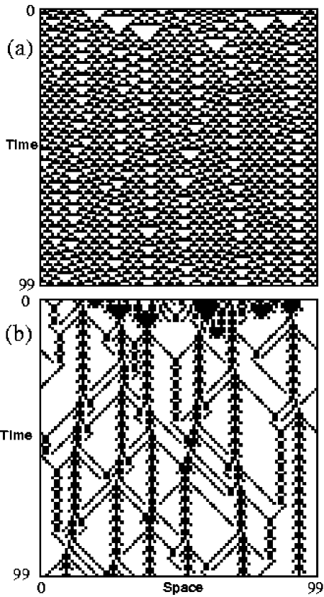
FIG. 2.: (a) Raw space-time diagram and (b) filtered space-time diagram of ECA 54 behavior starting from an arbitrary initial configuration. After [22].

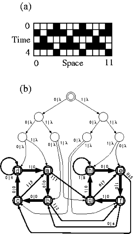
FIG. 3.: (a) Space-Time patch of ECA54’s primary domain $\Lambda$. (b) The transducer that recognizes $\Lambda$ and deviations from it. After [22].

The analysis in [22] identified $7$ dominant two- and three-particle interactions. We now analyze just one: the $\gamma^{+}+\gamma^{-}\rightarrow\beta$ interaction to illustrate the importance of a particle’s intrinsic periodicity.

Naive analysis would simply look at the space-time diagram, either the raw or filtered ones in Fig. 2, and conclude that these particles had periodicities $P(\gamma^{+})=P(\gamma^{-})=1$. Plugging this and the other data—$T(\Lambda)=2$, $S(\Lambda)=4$, and $\Delta v=2$—leads to upper bound $n_{\alpha,\beta}=1/4$! This is patently wrong; it’s not even an integer.

Figure 4 gives the transducer-filtered space-time diagram for the $\gamma^{+}$ and $\gamma^{-}$ particles. The domain $\Lambda$ is filtered out, as above. In the filtered diagrams the transducer state reached on scanning the particle wedge cells is indicated.

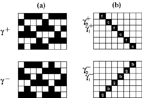
FIG. 4.: The transducer-filtered space-time diagrams for the $\gamma^{+}$ and $\gamma^{-}$ particles. (a) The raw space-time patches containing the particles. (b) The same patches with the $\Lambda$ filtered out. The cells not in $\Lambda$ are denoted in black; those in $\Lambda$ in white. In the filtered diagrams the transducer state reached on scanning the particle wedge cells is indicated. After [22].

From the space-time diagrams of Fig. 4(b) one notes that the transducer-state labeled wedges for each particle indicate that their intrinsic periodicities are $P(\gamma^{+})=2$ and $P(\gamma^{-})=2$. Then, from Thm. 22 we have that $n_{\alpha,\beta}=1$. That is, there is at most one product of these particles’ interaction.

Fig. 5 gives the transducer-filtered space-time diagram for the $\gamma^{+}+\gamma^{-}\rightarrow\beta$ interaction. A complete survey of all possible $\gamma^{+}$-$\Lambda$-$\gamma^{-}$ initial particle configurations shows that this is the only interaction for these particles. Thus, the upper bound is saturated.

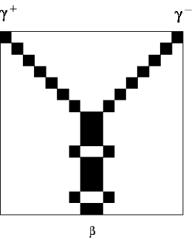
FIG. 5.: The transducer-filtered space-time diagrams for the $\gamma^{+}+\gamma^{-}\rightarrow\beta$ interaction. After [22].

B An Evolved CA

The second example for which we test the upper bound is a CA that was evolved by a genetic algorithm to perform a class of spatial computations: from all random initial configurations, synchronize within a specified number of iterations. This CA is $\phi_{sync_{1}}$ of [38]: a binary, radius-$3$ CA. The $128$-bit look-up table for $\phi_{sync_{1}}$ is given in Table I.

Here we are only interested in locally analyzing the various pairwise particle interactions observed in $\phi_{sync_{1}}$. It turned out that this CA used a relatively simple set of domains, particles, and interactions. Its particle catalog is given in Table II.

As one example, the two particles $\alpha$ and $\beta$ and the intervening domain $\Lambda$ have the properties given in Table II. From this data, Thm. 22 tells us that there is at most one interaction product:

$$n_{\alpha,\beta}=\frac{4\cdot 2\cdot\frac{1}{4}}{2\cdot 1}=1~{}.$$ (30)

$\phi$	Look-up Table (hexadecimal)
$\phi_{sync_{1}}$	F8A19CE6B65848EA
	D26CB24AEB51C4A0
$\phi_{parent}$	CEB2EF28C68D2A04
	E341FAE2E7187AE8

TABLE I.: Lookup tables (in hexadecimal) for $\phi_{sync_{1}}$ and $\phi_{parent}$. To recover the 128-bit string giving the CA look-up table output bits $s_{t+1}$, expand each hexadecimal digit (the first row followed by the second row) to binary. The output bits $s_{t+1}$ are then given in lexicographic order starting from the all-$0$s neighborhood at the leftmost bit in the 128-bit string.

The single observed interaction between the $\alpha$ and $\beta$ particles is shown in Fig. 6. As this space-time diagram shows, the interaction creates another $\beta$ particle, i.e., $\alpha+\beta\rightarrow\beta$. An exhaustive survey of the $8$ ($=4\times 2$) possible particle-phase configurations shows that this is the only interaction for these two particles. Thus, in this case, we see that Thm. 22 again gives a tight bound; it cannot be reduced.

$\phi_{sync_{1}}$ Particle Catalog
Domains ${\boldsymbol{\Lambda}}$
Name	Regular language		$T(\Lambda)$	$S(\Lambda)$
$\Lambda$	$0^{4}0^{*}$, $1^{4}1^{*}$		2	1
Particles P
Name	Wall	$P$	$d$	$v$
$\alpha$	$\Lambda_{j}\Lambda_{j}$	4	-1	-1/4
$\beta$	$\Lambda_{j}\Lambda_{1-j}$	2	-1	-1/2
$\gamma$	$\Lambda_{j}\Lambda_{j}$	8	-1	-1/8
$\delta$	$\Lambda_{j}\Lambda_{j}$	2	0	0
Interactions I
Type	Interaction		Interaction
React	$\alpha+\beta\rightarrow\beta$		$\gamma+\beta\rightarrow\beta$
React	$\delta+\beta\rightarrow\beta$		$\gamma+\alpha\rightarrow\alpha$
React	$\delta+\alpha\rightarrow\alpha$		$\delta+\gamma\rightarrow\alpha$

TABLE II.: The particle catalog of $\phi_{sync_{1}}$. $\Lambda_{j}$, $j\in\{0,1\}$, indicates the two temporal phases of domain $\Lambda$.

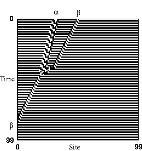
FIG. 6.: The interaction between an $\alpha$ and a $\beta$ particle in $\phi_{sync_{1}}$.

C Another Evolved CA

The third, more complicated example is also a CA that was evolved by a genetic algorithm to synchronize. This CA is $\phi_{parent}$ of [53]. It too is a binary radius-3 CA. The $128$-bit look-up table for $\phi_{parent}$ was given in Table I.

Here the two particles $\alpha$ and $\beta$ and the intervening domain $\Lambda$ have the properties given in Table III. Note that this is the same domain as in the preceding example.

$\phi_{parent}$ Particle Properties
Domain	$T$	$S$
$\Lambda$	2	1
Particle	$P$	$d$	$v$
$\alpha$	8	2	1/4
$\beta$	2	-3	-3/2

TABLE III.: Properties of two of $\phi_{parent}$’s particles.

From this data, Thm. 22 now says that there are at most:

$$n_{\alpha,\beta}=\frac{8\cdot 2\cdot\frac{7}{4}}{2\cdot 1}=14$$ (31)

interactions.

Of these 14 input configurations, it turns out several give rise to the same products. From a complete survey of $\alpha$-$\Lambda$-$\beta$ configurations, the result is that there are actually only $4$ different products from the $\alpha+\beta$ interaction; these are:

$$\alpha+\beta \rightarrow \emptyset$$

$$\alpha+\beta \rightarrow \gamma$$

$$\alpha+\beta \rightarrow 2\beta$$

$$\alpha+\beta \rightarrow \beta+\alpha$$

They are shown in Fig. 7.

This example serves to highlight the distinction between the maximum number of interaction configurations, as bounded by Thm. 22, and the actual number of unique products of the interaction. We shall return to this distinction later on.

FIG. 7.: The four different (out of 14 possible) interaction products for the $\alpha+\beta$ interaction.

D ECA 110

In the next example, we test Thm. 22 on one of the long-appreciated “complex” CA, elementary CA 110. As long ago as 1986, Wolfram [10, Appendix 15] conjectured that this rule is able to support universal, Turing-equivalent computation (replacing an earlier dictum [42, p. 31] that all elementary CA are “too simple to support universal computation”). While this conjecture initially excited little interest, in the last few years it has won increasing acceptance in the CA research community. Though to date there is no published proof of universality, there are studies of its unusually rich variety of domains and particles, one of the most noteworthy of which is McIntosh’s work on their tiling and tessellation properties [54]. Because of this CA’s behavioral richness, we do not present its complete particle catalog and computational-mechanical analysis here; rather see [55]. Instead, we confine ourselves to a single type of reaction where the utility of our upper bound theorem is particularly notable.

We consider one domain, labeled $\Lambda^{0}$, and two particles that move through it, called $\beta$ and $\kappa$ [55]. (This $\beta$ particle is not to be confused with the $\beta$ of our previous examples.) $\Lambda^{0}$ is ECA 110’s “true vacuum”: the domain that is stable and overwhelmingly the most prominent in space-time diagrams generated from random samples of initial configurations. It has a temporal period $T(\Lambda^{0})=1$, but a spatial period $S(\Lambda^{0})=14$. The $\beta$ particle has a period $P(\beta)=15$, during the course of which it moves four steps to the left: $d_{\beta}=4$. The $\kappa$ particle, finally, has a period $P(\kappa)=42$, and moves $d_{\kappa}=14$ steps to the left during its cycle. This data gives the $\beta$ particle a velocity of $v_{\beta}=-4/15$ and the $\kappa$ particle $v_{\kappa}=-1/3$.

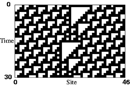
FIG. 8.: The particle $\beta$ of ECA 110: The space-time patch shows two complete cycles of particle phase.

Naively, one would expect to have to examine $630$ ($=P(\beta)P(\kappa)=15\times 42$) different particle-phase configurations to exhaust all possible interactions. Theorem 22, however, tells us that all but

$${(15)(42)({-4\over 15}-{-1\over 3})\over(14)(1)}=3$$ (32)

of those initial configurations are redundant. In fact, an exhaustive search shows that there are exactly three distinct interactions:

$$\beta+\kappa \rightarrow \alpha+3w_{right}~{},$$

$$\beta+\kappa \rightarrow \beta+4w_{right}~{},$$

$$\beta+\kappa \rightarrow \eta~{}.$$

Here, $\alpha$, $w_{right}$, and $\eta$ are additional particles generated by ECA 110. These interactions are depicted, respectively, in Figures 11, 10, and 12.

We should note that the $w_{right}$ particle is somewhat unusual in that several can propagate side by side, or even constitute a domain of their own. There are a number of such “extensible” particle families in ECA 110 [55].

FIG. 9.: The particle $\kappa$ of ECA 110: The space-time diagram shows one complete cycle of particle phase.

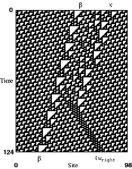
FIG. 10.: The reaction $\beta+\kappa\rightarrow\beta+4w_{right}$ in ECA 110.

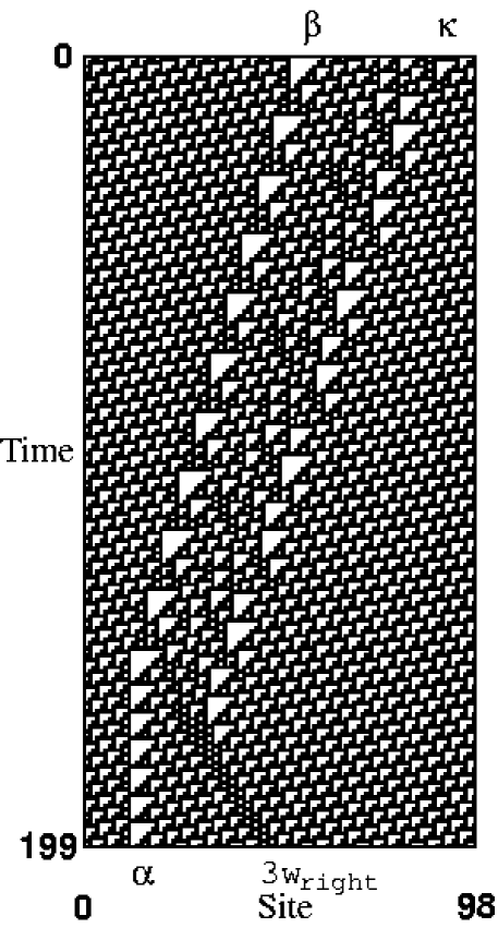
FIG. 11.: The reaction $\beta+\kappa\rightarrow\alpha+3w_{right}$ in ECA 110.

We again see, in this complex case, that the bound of Thm. 22 is attained.

VIII Conclusion

A Summary

The original interaction product formula of [9] is limited to particles propagating in a completely uniform background; i.e., to a domain whose spatial and temporal periods are both $1$. When compared to the rich diversity of domains generated by CAs, this is a considerable restriction, and so the formula does not help in analyzing many CAs. We have generalized the original result and along the way established a number of properties of domains and particles—structures defined by CA computational mechanics. The examples showed that the upper bound is tight and that, in complex CAs, particle interactions are substantially less complicated than they look at first blush. Moreover, in developing the bound for complex domains, the analysis elucidated the somewhat subtle notion of a particle’s intrinsic periodicity—a property not apparent from the CA’s raw space-time behavior: it requires rather an explicit representation of the bordering domains’ structure.

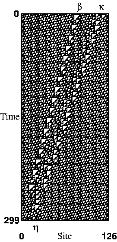
FIG. 12.: The reaction $\beta+\kappa\rightarrow\eta$ in ECA 110.

Understanding the detailed structure of particles and their interactions moves us closer to an engineering discipline that would tell one how to design CA to perform a wide range of spatial computations using various particle types, interactions, and geometries. In a complementary way, it also brings us closer to scientific methods for analyzing the intrinsic computation of spatially extended systems [55].

B Open Problems

The foregoing analysis merely scratches the surface of a detailed analytical approach to CA particle “physics”: Each CA update rule specifies a microphysics of local (cell-to-cell) space and time interactions for its universe; the goal is to discover and analyze those emergent structures that control the macroscopic behavior. For now, we can only list a few of the open, but seemingly accessible, questions our results suggest.

It would be preferable to directly calculate the number of products coming out of the interaction region, rather than (as here) the number of distinct particle-domain-particle configurations coming into the interaction region. We believe this is eminently achievable, given the detailed representations of domain and particles that are entailed by a computational mechanics analysis of CAs.

Two very desirable extensions of these results suggest themselves. The first is to go from strictly periodic domains to cyclic (periodic and “chaotic”) domains and then to general domains. The principle difficulty here is that Prop. 1 plays a crucial role in our current proof, but we do not yet see how to generalize its proof to chaotic (positive entropy density) domains. The second extension would be to incorporate aperiodic particles, such as the simple one exhibited by ECA 18 [56]. We suspect this will prove considerably more difficult than the extension to cyclic domains: it is not obvious how to apply notions like “particle period” and “velocity” to these defects. A third extension, perhaps more tractable than the last, is to interactions of more than two particles. The geometry and combinatorics will be more complicated than in the two-particle case, but we conjecture that it will be possible to establish an upper bound on the number of interaction products for $n-$particle interactions via induction.

Does there exist an analogous lower bound on the number of interactions? If so, when do the upper and lower bounds coincide?

In solitonic interactions the particle number is preserved [3, 8, 9, 33, 57]. What are the conditions on the interaction structure that characterize solitonic interactions? The class of soliton-like particles studied in [9] possess a rich “thermodynamics” closely analogous to ordinary thermodynamics, explored in detailed in [58]. Do these results generalize to the broader class of domains and particles, as the original upper bound of [9] does?

While the particle catalog for ECA 110 is not yet provably complete, for every known pair of particles the number of distinct interaction products is exactly equal to the upper bound given by our theorem. This is not generally true of most of the CAs we have analyzed and is especially suggestive in light of the widely-accepted conjecture that the rule is computation universal. We suspect that ECA 110’s fullness or behavioral flexibility is connected to its computational power. (Cf. Remark 2 to Thm. 22.) However, we have yet to examine other, computation universal CA to see whether they, too, saturate the bound of our theorem. One approach to this question would be to characterize the computational power of systems employing different kinds of interactions, as is done in [59] for computers built from interacting (continuum) solitary waves.

Proof of Lemma 1

Lemma 1

If a domain $\Lambda^{i}$ has a periodic phase, then the domain is periodic, and the spatial periodicities $S(\Lambda^{i}_{j})$ of all its phases $\Lambda^{i}_{j},j=0,\ldots,p-1,$ are equal.

Proof. The proof consists of two parts. First, and most importantly, it is proved that the spatial periodicities of the temporal phases of a periodic domain $\Lambda^{i}$ cannot increase and that the periodicity of one phase implies the periodicity of all its successors. Then it follows straightforwardly that the spatial periodicities have to be equal for all temporal phases and that they all must be periodic.

Our proof employs the update transducer $T_{\phi}$, which is simply the FST which scans across a lattice configuration and outputs the effect of applying the CA update rule $\phi$ to it. For reasons of space, we refrain from giving full details on this operator—see rather [21]. Here we need the following results. If $\phi$ is a binary, radius-$r$ CA, the update transducer has $2^{2r}$ states, representing the $2^{2r}$ distinct contexts (words of previously read symbols) in which $T_{\phi}$ scans new sites, and we customarily label the states by these context words. The effect of applying the CA $\phi$ to a set of lattice configuration represented by the DFA $M$ is a new machine, given by $T_{\phi}M$—the “direct product” of the machines $M$ and $T_{\phi}$. Once again, for reasons of space, we will not explain how this direct product works in the general case. We are interested merely in the special case where $M=\Lambda^{i}_{j}$, the $j^{th}$, periodic phase of a domain, with spatial period $n$. The next phase of the domain, $\Lambda^{i}_{j+1}$, is the composed automaton $T_{\phi}M$, once the latter has been minimized. Before the latter step $T_{\phi}M$ consists of $n$ “copies” of the FST $T_{\phi}$, one for each of $\Lambda^{i}_{j}$’s $n$ states. There are no transitions within a copy. Transitions from copy $k$ to copy $k^{\prime}$ occur only if $k^{\prime}=k+1$ ($\bmod~{}n$). In total, there are $n{2}^{2r}$ states in the direct composition.

$T_{\phi}M$ is finite and deterministic, but far from minimal. We are interested in its minimal equivalent machine, since that is what we have defined as the representative of the next phase of the domain. The key to our proof is an unproblematic part of the minimization, namely, removing states that have no predecessors (i.e., no incoming transitions) and so are never reached. (Recall that, by hypothesis, we are examining successive phases of a domain, all represented by strongly connected process graphs.) It can be shown, using the techniques in [21], that if the transition from state $k$ in $\Lambda^{i}_{j}$ to state $k+1$ occurs on a $0$ (respectively, on a $1$), then in the composed machine, the transitions from copy $k$ of $T_{\phi}$ only go to those states in copy $k+1$ whose context string ends in a $0$ (respectively, in a $1$). Since states in copy $k+1$ can be reached only from states in copy $k$, it follows that half of the states in each copy cannot be reached at all, and so they can be eliminated without loss.

Now, this procedure of eliminating states without direct predecessors in turn leaves some states in copy $k+2$ without predecessors. So we can re-apply the procedure, and once again, it will remove half of the remaining states. This is because applying it twice is the same as removing those states in copy $k+2$ for which the last two symbols in the context word differ from the symbols connecting state $k$ to state $k+1$ and state $k+1$ to state $k+2$ in the original domain machine $\Lambda^{i}_{j}$.

What this procedure does is exploit the fact that, in a domain, every state is encountered only in a unique update-scanning context; we are eliminating combinations of domain-state and update-transducer-state that simply cannot be reached. Observe that we can apply this procedure exactly $2r$ times, since that suffices to establish the complete scanning context, and each time we do so, we eliminate half the remaining states. We are left then with $n{2}^{2r}/2^{2r}=n$ states after this process of successive halvings. Further observe that, since each state $k$ of the original domain machine $\Lambda^{i}_{j}$ occurs in some scanning context, we will never eliminate all the states in copy $k$. Since each of the $n$ copies has at least one state left in it, and there are only $n$ states remaining after the halvings are done, it follows that each copy contains exactly one state, which has one incoming transition, from the previous copy, and one outgoing transition, to the next copy. The result of eliminating unreachable states, therefore, is a machine of $n$ states which is not just deterministic but (as we have defined the term) periodic. Note, however, that this is not necessarily the minimal machine, since we have not gone through a complete minimization procedure, merely the easy part of one. $\Lambda^{i}_{j+1}$ thus might have fewer than $n$ states, but certainly no more.

To sum up: We have established that, if $\Lambda^{i}_{j}$ is a periodic domain phase, then $\Lambda^{i}_{j+1}$ is also periodic and $S(\Lambda^{i}_{j+1})\leq S(\Lambda^{i}_{j})$. Thus, for any $t$, $S(\boldsymbol{\Phi}^{t}\Lambda^{i}_{j})\leq S(\Lambda^{i}_{j})$. But $\boldsymbol{\Phi}^{t}\Lambda^{i}_{j})=\Lambda^{i}_{(j+t)\bmod p}$ and if $t=p$, we have $\Lambda^{i}_{(j+t)\bmod p}=\Lambda^{i}_{(j+p)\bmod p}=\Lambda^{i}_{j}$. Putting these together we have

$$S(\Lambda^{i}_{j+1})\leq S(\Lambda^{i}_{j})\Rightarrow S(\Lambda^{i}_{j+1})=S(\Lambda^{i}_{j})~{},$$ (33)

for $j=0,1,\ldots,p-1$. This implies that the spatial period is the same, namely $n$, for all phases of the domain. And this proves the proposition when the CA alphabet is binary.

The reader may easily check that a completely parallel argument holds if the CA alphabet is not binary but $m-$ary, substituting $m$ for 2 and $(m-1)/m$ for $1/2$ in the appropriate places. We omit it here for reasons of space and notational complexity. $\Box$

REFERENCES

- [1] A. W. Burks (Ed.), Essays on Cellular Automata, University of Illinois Press, Urbana, 1970.
- [2] E. R. Berlekamp, J. H. Conway, R. K. Guy, Winning Ways for your Mathematical Plays, Academic Press, New York, 1982.
- [3] M. Peyrard, M. D. Kruskal, Kink dynamics in the highly discrete sine-Gordon system, Physica D 14 (1984) 88–102.
- [4] P. Grassberger, New mechanism for deterministic diffusion, Physical Review A 28 (1983) 3666–7.
- [5] N. Boccara, J. Nasser, M. Roger, Particle-like structures and their interactions in spatio-temporal patterns generated by one-dimensional deterministic cellular automaton rules, Physical Review A 44 (1991) 866 – 875.
- [6] N. Boccara, M. Roger, Block transformations of one-dimensional deterministic cellular automata, Journal of Physics A 24 (1991) 1849 – 1865.
- [7] N. Boccara, Transformations of one-dimensional cellular automaton rules by translation-invariant local surjective mappings, Physica D 68 (1993) 416–426.
- [8] Y. Aizawa, I. Nishikawa, K. Kaneko, Soliton turbulence in cellular automata, in: H. Gutowitz (Ed.), Cellular Automata: Theory and Experiment, MIT Press, Cambridge, Massachusetts, 1991, pp. 307–327, also published as Physica D 45 (1990), nos. 1–3.
- [9] J. K. Park, K. Steiglitz, W. P. Thurston, Soliton-like behavior in automata, Physica D 19 (1986) 423–432.
- [10] S. Wolfram (Ed.), Theory and Applications of Cellular Automata, World Scientific, Singapore, 1986.
- [11] S. Wolfram, Cellular Automata and Complexity: Collected Papers, Addison-Wesley, Reading, Massachusetts, 1994, online at http://www.stephenwolfram.com/publications/books/ ca-reprint/.
- [12] K. Lindgren, M. G. Nordahl, Universal computation in a simple one-dimensional cellular automaton, Complex Systems 4 (1990) 299–318.
- [13] J. P. Crutchfield, M. Mitchell, The evolution of emergent computation, Proceedings of the National Academy of Sciences 92 (1995) 10742–10746.
- [14] J. B. Yunes, Seven-state solutions to the firing squad synchronization problem, Theoretical Computer Science 127 (1994) 313–332.
- [15] K. Eloranta, Partially permutive cellular automata, Nonlinearity 6 (1993) 1009–1023.
- [16] K. Eloranta, The dynamics of defect ensembles in one-dimensional cellular automata, Journal of Statistical Physics 76 (1994) 1377–1398.
- [17] K. Eloranta, E. Nummelin, The kink of cellular automaton rule 18 performs a random walk, Journal of Statistical Physics 69 (1992) 1131–1136.
- [18] P. Manneville, N. Boccara, G. Y. Vichniac, R. Bidaux (Eds.), Cellular Automata and Modeling of Complex Systems: Proceedings of the Winter School, Les Houches, France, February 21–28, 1989, Vol. 46 of Springer Proceedings in Physics, Springer-Verlag, Berlin, 1990.
- [19] D. Andre, F. H. Bennett, III, J. R. Koza, Evolution of intricate long-distance communication signals in cellular automata using genetic programming, in: C. G. Langton, K. Shimohara (Eds.), Artificial Life V, MIT Press, Cambridge, Massachusetts, 1997, pp. 513–520.
- [20] J. E. Hanson, J. P. Crutchfield, The attractor-basin portrait of a cellular automaton, Journal of Statistical Phyics 66 (1992) 1415–1462.
- [21] J. E. Hanson, Computational mechanics of cellular automata, Ph.D. thesis, University of California, Berkeley (1993).
- [22] J. E. Hanson, J. P. Crutchfield, Computational mechanics of cellular automata: An example, Physica D 103 (1997) 169–189.
- [23] D. Eppstein, Gliders in life-like cellular automata, Interactive online database of two-dimensional cellular automata rules with gliders, http://fano.ics.uci.edu/ca/.
- [24] P. Manneville, Dissipative Structures and Weak Turbulence, Academic Press, Boston, Massachusetts, 1990.
- [25] M. C. Cross, P. Hohenberg, Pattern Formation Out of Equilibrium, Reviews of Modern Physics 65 (1993) 851–1112.
- [26] A. T. Winfree, The Geometry of Biological Time, Springer-Verlag, Berlin, 1980.
- [27] A. T. Winfree, When Time Breaks Down: The Three-Dimensional Dynamics of Electrochemical Waves and Cardiac Arrhythmias, Princeton University Press, Princeton, 1987.
- [28] E. Infeld, G. Rowlands, Nonlinear Waves, Solitions, and Chaos, Cambridge University Press, Cambridge, England, 1990.
- [29] W. Poundstone, The Recursive Universe: Cosmic Complexity and the Limits of Scientific Knowledge, William Morrow, New York, 1984.
- [30] D. Griffeath, Additive and Cancellative Interacting Particle Systems, Vol. 724 of Lecture Notes in Mathematics, Springer-Verlag, Berlin, 1979.
- [31] T. M. Liggett, Interacting Particle Systems, Springer-Verlag, Berlin, 1985.
- [32] D. H. Rothman, S. Zaleski, Lattice-Gas Cellular Automata: Simple Models of Complex Hydrodynamics, Vol. 5 of Collection Aléa Saclay, Cambridge University Press, Cambridge, England, 1997.
- [33] K. Steiglitz, I. Kamal, A. Watson, Embedding computation in one-dimensional automata by phase coding solitons, IEEE Transactions on Computers 37 (1988) 138–144.
- [34] D. Griffeath, C. Moore, Life without death is P-complete, Complex Systems 10 (1996) 437–447.
- [35] C. Moore, Majority-vote cellular automata, Ising dynamics, and P-completeness, Journal of Statistical Physics 88 (1997) 795–805.
- [36] C. Moore, M. G. Nordahl, Lattice gas prediction is P-complete, Electronic pre-preprint, arxiv.org, comp-gas/9704001 (1997).
- [37] R. Das, M. Mitchell, J. P. Crutchfield, A genetic algorithm discovers particle computation in cellular automata, in: Y. Davidor, H.-P. Schwefel, R. Manner (Eds.), Proceedings of the Conference on Parallel Problem Solving in Nature — PPSN III, Lecture Notes in Computer Science, Springer-Verlag, Berlin, 1994, pp. 344–353.
- [38] W. Hordijk, M. Mitchell, J. P. Crutchfield, Mechanisms of emergent computation in cellular automata, in: A. E. Eiben, T. Bäck, M. Schoenaur, H.-P. Schwefel (Eds.), Parallel Problem Solving in Nature—PPSN V, Lecture Notes in Computer Science, Springer-Verlag, Berlin, 1998, pp. 613–622.
- [39] N. Margolus, Crystalline computation, in: A. J. G. Hey (Ed.), Feynman and Computation: Exploring the Limits of Computers, Perseus Books, Reading, Massachusetts, 1999, pp. 267–305, e-print, arxiv.org, comp-gas/9811002.
- [40] R. Das, The evolution of emergent computation in cellular automata, Ph.D. thesis, Colorado State University (1996).
- [41] W. Hordijk, Dynamics, emergent computation, and evolution in cellular automata, Ph.D. thesis, University of New Mexico, Albuquerque, New Mexico, online at http://www.santafe.edu/projects/ evca/ Papers/ WH-Diss.html (1999).
- [42] S. Wolfram, Universality and complexity in cellular automata, Physica D 10 (1984) 1–35, reprinted in [11].
- [43] J. P. Crutchfield, Is anything ever new? Considering emergence, in: G. Cowan, D. Pines, D. Melzner (Eds.), Complexity: Metaphors, Models, and Reality, Vol. 19 of Santa Fe Institute Studies in the Sciences of Complexity, Addison-Wesley, Reading, Massachusetts, 1994, pp. 479–497.
- [44] J. H. Holland, Emergence: From Chaos to Order, Addison-Wesley, Reading, Massachusetts, 1998.
- [45] A. Wuensche, Classifying cellular automata automatically: Finding gliders, filtering, and relating space-time patterns, attractor basins, and the Z parameter, Complexity 4 (1999) 47–66.
- [46] D. Eppstein, Searching for spaceships, E-print, arxiv.org, cs.AI/0004003 (2000).
- [47] S. Wolfram, Statistical mechanics of cellular automata, Reviews of Modern Physics 55 (1983) 601–644, reprinted in [11].
- [48] S. Wolfram, Computation theory of cellular automata, Communications in Mathematical Physics 96 (1984) 15–57, reprinted in [11].
- [49] J. E. Hopcroft, J. D. Ullman, Introduction to Automata Theory, Languages, and Computation, Addison-Wesley, Reading, 1979, 2nd edition of Formal Languages and Their Relation to Automata, 1969.
- [50] J. P. Crutchfield, K. Young, Inferring statistical complexity, Physical Review Letters 63 (1989) 105–108.
- [51] J. P. Crutchfield, J. E. Hanson, Turbulent pattern bases for cellular automata, Physica D 69 (1993) 279–301.
- [52] D. M. Burton, Elementary Number Theory, Allyn and Bacon, Boston, 1976.
- [53] J. P. Crutchfield, W. Hordijk, M. Mitchell, Computational performance of evolved cellular automata: Parts I and II, manuscript in preparation.
- [54] H. V. McIntosh, Rule 110 as it relates to the presence of gliders, Electronic manuscript, http://delta.cs.cinvestav.mx/mcintosh/comun/ RULE110W/RULE110.html (2000).
- [55] J. P. Crutchfield, C. R. Shalizi, Intrinsic computation versus engineered computation: The computational mechanics of rule 110, manuscript in preparation.
- [56] J. P. Crutchfield, J. E. Hanson, Attractor vicinity decay for a cellular automaton, Chaos 3 (1993) 215–224.
- [57] M. J. Ablowitz, M. D. Kruskal, J. F. Ladik, Solitary wave collisons, SIAM Journal on Applied Mathematics 36 (1979) 428–437.
- [58] C. H. Goldberg, Parity filter automata, Complex Systems 2 (1988) 91–141.
- [59] M. H. Jakubowski, K. Steiglitz, R. Squier, Information transfer between solitary waves in the saturable Schrödinger equation, Physical Review E 56 (1997) 7267–7272.