Amplitude measurements of Faraday waves

Abstract

A light reflection technique is used to measure quantitatively the surface elevation of Faraday waves. The performed measurements cover a wide parameter range of driving frequencies and sample viscosities. In the capillary wave regime the bifurcation diagrams exhibit a frequency independent scaling proportional to the wavelength. We also provide numerical simulations of the full Navier-Stokes equations, which are in quantitative agreement up to supercritical drive amplitudes of $\varepsilon\simeq 20\%$. The validity of an existing perturbation analysis is found to be limited to $\varepsilon<2.5\%$.

I Introduction

A sound understanding of hydrodynamic pattern forming systems is based on a balanced interplay between experiment and theory, both analytical and numerical. During the past this concept has led to considerable progress, especially in case of Rayleigh-Bénard convection (RBC) or Taylor-Couette flow (TCF), where an amazing level of quantitative agreement has been achieved. Another famous example of pattern forming systems is the Faraday experiment: Surface waves on a free liquid-air or liquid-liquid interface are excited by a sinusoidal vibration of the fluid layer in vertical direction. This system has the advantage of fairly short time scales in combination with a very rich bifurcation behavior. During the last two decades the focus in this field was on nonlinear pattern selection [1, 2, 3, 4, 5], secondary instabilities [6], the transition towards chaos [7], droplet ejection [8] and stokes drift [9]. However, due to the parametric drive mechanism the mathematical description of the Faraday experiment is more complicated as compared to RBC or TCF and the quantitative understanding is less advanced yet. For instance, it was not until recently that a rigorous linear stability theory had been developed, valid for viscous fluids and realistic boundary conditions[10]. Nowadays the predictions of the linear theory and the experimental results agree within a few percent [11]. On the non-linear level, however, the agreement between theory and experiment can at best be considered qualitative: In the framework of a weakly non-linear perturbation analysis different primary surface wave patterns with quadratic, hexagonal etc. symmetry have been predicted [12]. Even though most of them have been found in experiments [4, 5], empiric and predicted phase diagram reveal only a qualitatitve coincidence. Moreover, other experiments operate with a two-frequency drive signal [13, 14], or at very shallow filling heights [15] or with complex fluids [16, 17, 18]. The resulting pattern dynamics becomes more complex and exotic structures like superlattices [14, 15, 17] or oscillons [18] appear. In some cases a qualitative understanding based on symmetry arguments could be obtained [15, 19].

With regard to this situation it comes as a surprise that a systematic quantitative investigation of the system’s major order parameter, the surface elevation, has not been undertaken yet. Such data is indispensable for a verification of any nonlinear theory. It is the aim of the present work to provide extensive experimental material in order to fill this gap. A measurement technique is presented appropriate to quantify the surface elevation of Faraday ripples. Our measurements cover a broad part of the parameter space explored in recent experiments on pattern selection in the Faraday experiment. In case of low viscosity fluids our findings are expected to compare with the perturbation analysis of Zhang and Vinãls [12] – at least at a weak supercritical drive. Furthermore, a closer comparison yields a reliable estimate of the validity range of this approximation. Farther away from threshold of the instability, quantitative theoretical predictions are not available yet. Here we provide a numerical simulation by means of a finite difference scheme. This computation allows for 2-dimensional solutions of the full Navier-Stokes equations. They are used for a comparison with our measurements on line patterns.

II The system

We consider a fluid layer of thickness $h$ with a free surface vibrated in vertical direction at a drive frequency $\Omega$. In the frame of reference co-moving with the container the liquid is subject to a modulated gravity acceleration ${\rm g}+a\,\sin{(\Omega t)}$, where ${\rm g}$ is the gravitational acceleration and $a$ the amplitude of the drive. The fluid, considered as being incompressible, is characterized by the kinematic viscosity $\nu$, the density $\rho$, and the surface tension $\sigma$. The hydrodynamic problem is governed by the Navier-Stokes equation, in which the modulated gravity enters as a parametric drive. The boundary conditions are free slip at the fluid-air interface and no slip along the walls and the bottom of the container. If $a$ exceeds a critical threshold $a_{c}(\Omega,h,\nu,\rho,\sigma)$ the surface, being plane at the beginning, undergoes the Faraday instability and standing waves with a wavenumber $k$ appear. Usually these waves organize themselves in form of regular patterns of different possible symmetries (lines, squares, hexagons …). In containers with a large lateral aspect ratio (the ratio between container dimension to wavelength of the pattern) the pattern selection is geometry independent and solely governed by the nonlinearities in the equations of motion. In contrast, by changing the lateral container extension one can manipulate the selection process. For instance, by reducing one sidelength of a beforehand quadratic container, a line pattern (oriented parallel to the shorter side) can eventually be enforced in a situation where squares would prevail otherwise. In the present paper extensive use will be made of this geometrical selection feature.

Generically, the time dependence of the Faraday mode bifurcating out of the undisturbed plane surface is subharmonic, i.e. the surface oscillates at half the drive frequency $\omega=\Omega/2$. The standing wave surface profile $\eta({\bf r})$ at onset of the instability can be written in the form

$$\eta_{N}({\bf r},t)=\frac{1}{2}\,\sum_{i=1}^{N}{(A_{i}e^{{\rm i}{\bf k}_{i}\cdot{\bf r}}}+c.c.)\,\sum_{n=-\infty}^{+\infty}\zeta_{n}e^{{\rm i}n\frac{\Omega}{2}t}.$$ (1)

Here ${\bf r}=(x,y)$ abbreviates the horizontal coordinates. The set of Fourier coefficients $\{\zeta_{n}\}$ determines the subharmonic time dependence. Exactly at the onset of the instability, $a=a_{c}$, one has $\zeta_{n}=0$ for even $n$, while the odd coefficients are the components of the eigenvector related to the linear stability problem. The spatial modes are characterized by the wave vectors ${\bf k}_{i}$, each carrying an individual amplitude $A_{i}$. These quantities are determined by the nonlinearities of the problem and – if appropriate – also by the container geometry. In principle the ${\bf k}_{i}$ can have any length and orientation but usually they are supposed to be equally spaced on the circle $|{\bf k}_{i}|=k$. Then the number $N$ of participating modes determines the degree of rotational symmetry of the pattern: $N=1$ corresponds to lines, $N=2$ to squares, $N=3$ to hexagons or triangles, etc. Patterns with $N>3$ are no longer translational symmetric, we refer to them as quasi-periodic.

III Prework by other authors

A Experimental

There exist a considerable number of measuring techniques appropriate to investigate the surface wave dynamics. They range from contacting permittivity measurements [20] over optical systems [21] including interferometry, radar back scattering [22] up to x-ray absorption techniques [23]. Most of these procedures apply to gravity waves, i.e. long wavelength surface waves. Each of them has its own limitations. Either the amplitude is recorded locally in space, or the detector is too slow to resolve the temporal spectrum. One of the strongest restrictions for optical reflection techniques comes from the poor reflectivity of most fluid-air interfaces. Only a few percent of the incident light is reflected and an even smaller contribution is due to diffusive back-scattering. Since the latter is crucial for standard visualization techniques such as holographic photography or triangulation[24], these methods often do not work properly. One might think of spraying the fluid surface with tracer particles like club moss seeds but this in turn affects the surface tension or the surface viscosity in an uncontrollable manner. In a pair of very recent publications [25, 26] the authors propose sophisticated methods based on a colored illumination or on an array of microlenses. A standard visualization technique used in several Faraday experiments is the light shadowgraphy [3, 4, 27]. A beam of parallel light with a diameter comparable to the container size passes through the fluid layer. The deformed standing wave surface pattern with its heaps and hollows acting like an array of collecting and diffusing lenses is mapped onto a screen. However, this technique is restricted to very small surface deformations for which the profile can be recovered by ray tracing. Otherwise caustics occur, which make this simple and effective method break down.

An alternative technique introduced by Wright, Budakin and Putterman [28] is based on intensity losses due to diffusive scattering. These authors use Polystyrene colloids to provide light scatterers within the fluid. The transversing light intensity, weakly modulated by the local layer thickness, is recorded by a high-sensitivity CCD-camera to reconstruct the surface profile. As an example, a snapshot is presented taken at a rather strong drive amplitude within the turbulent regime.

To our knowledge, previous quantitative investigations on near-onset Faraday waves are restricted to the low-frequency regime, i.e. below $\Omega\simeq 30{\rm Hz}$. Douady [29] presents an investigation, where the deflection of a thin laser beam directed onto a wave node is recorded. To prevent the nodes from a gradual drift, Douady uses the ”rimfull technique” to fix the position of the pattern relative to the container boundaries. That way the structure experiences a mode discretization dictated by the container geometry. Data for the elevation maxima and the linear relaxation time $\tau$ are provided for a silicone oil at a viscosity of $10{\rm cS}$ and drive frequencies between $20$ and $30{\rm Hz}$.

Several other authors report amplitude measurements in small aspect ratio experiments at driving frequencies between 5 and 10Hz [30, 31, 32]. In this situation a considerable mismatch between frequency and wavelength may occur. The resulting detuning renders the primary bifurcation hysteretic. An additional problem in these experiments is the moving contact line between the fluid and the container. It may also generate a hysteresis or even induce an irregular time dependent wave dynamics.

B Theoretical

1 Numerical

A couple of numerical simulations on Faraday waves is worth mentioning in the present context. Zhang and Vinãls [33] reduce the original full 3-dimensional hydrodynamic problem to a set of 2-dimensional non-local equations formulated in terms of the lateral coordinates only. This is the outcome of the so called ”quasi-potential approximation”, which considers the bulk flow as being potential (inviscid). Vortical flow contributions in the viscous boundary layer beneath the surface are accounted for by an effective boundary condition. Clearly this analysis is only valid for deep layers ($h\to\infty$) and restricted to the low dissipation limit $\nu k^{2}/\Omega\ll 1$. The derived equations for the surface elevation $\eta({\boldsymbol{r}},t)$ are numerically integrated by a pseudo-spectral algorithm. The principal concern of these simulations is to obtain the most preferred pattern and to investigate its resistance against secondary instabilities. Stationary patterns with different rotational symmetries have been observed. In particular, drive frequencies at the transition between gravity and capillary waves, $\Omega/2\pi\simeq 30{\rm Hz}$, give rise to the most interesting structures: Quasi-periodic pattern with a 10-fold rotational symmetry [4]. In the capillary regime squares or lines are observed depending on the viscosity of the sample fluid.

A somewhat different numerical procedure has been used by Schultz et al. [34] and Wright et al. [35]. Both investigations are based on the Euler equations for inviscid fluids. Dissipation is accounted for by a phenomenological linear damping term introduced afterwards. The numerical procedures used are respectively a boundary-integral method and a vortex-sheet technique. That way the profile of very steep 2-dimensional Faraday waves is investigated. Their findings comprise dimpled crests, the formation of a plumelike shape, or the beginning of droplet ejection.

Obviously, all of the aforementioned numerical work is restricted to the low dissipation limit and to large layer thicknesses. Indeed, we are not aware of systematic numerical simulations for viscous fluids on the basis of the full hydrodynamic equations and boundary conditions.

2 Analytical

The first step towards a theoretical understanding of pattern forming systems is a linear stability analysis. This gives access to the threshold amplitude $a_{c}$, the critical wave number $k_{c}$, and the most unstable mode. For mathematical convenience it is popular to assume laterally infinite geometries. Although it is known for a long time that the stability problem for Faraday waves can be approximately mapped to a parametrically driven pendulum [36] a rigorous stability analysis for viscous fluids dates back until recently [10]. Quantities evaluated by this method will be referred to in the following as ”results of the exact stability analysis”.

A nonlinear analysis suitable to predict the selected surface pattern just above the primary instability has been presented by Zhang and Vinãls [12]. They start form their reduced 2-dimensional set of quasi-potential equations (see Sec. III B 1) and perform a perturbation analysis for small supercritical drive $\varepsilon=(a-a_{c})/a_{c}\ll 1$. The analysis can be understood as a double expansion in $\varepsilon$ and in the dimensionless damping parameter $\gamma=\nu k^{2}/\Omega\ll 1$. Since $h\to\infty$ is assumed, vortical flow contributions coming from the viscous boundary layer along the bottom of the container are ignored. The pattern wavelength $2\pi/k$ is approximated by the inviscid dispersion relation

$$\left(\frac{\Omega}{2}\right)^{2}={\rm g}k+\frac{\sigma}{\rho}k^{3}.$$ (2)

In our experiments the damping parameter is $0.1<\gamma<0.2$ for the low viscosity sample S1 and lies between $1.3$ and $1.7$ for probe S2. Accordingly, the wave number $k$ evaluated by Eq. (2) for S1 agrees within $1\%$ with the result of the exact stability analysis but it is off by $20\%$ for S2. In the framework of the weakly non-linear analysis the surface profile is represented by Eq. (1) with $|k_{i}|=k_{c}$ and $\zeta_{n}=0$ for $n$ even. The mode amplitudes $A_{i}$ are governed by the set of the amplitude equations

$$\tau\partial_{t}A_{i}=\epsilon A_{i}-\sum_{j=1}^{N}\Gamma(\theta_{ij})|{A_{j}}|^{2}A_{i},$$ (3)

where $\tau$ is the time constant of linear damping, also an outcome of the linear analysis. $\Gamma(\theta)$ is the non-linear coupling function, whose dependence on the sample specifications and the drive frequency is analytically known. Evaluating $\Gamma$ at the angle increments $\theta_{ij}$ between two interacting modes ${\bf k}_{i}$ and ${\bf k}_{j}$ yields the set of cubic coupling coefficients, which governs the pattern selection process. By computing the stationary solutions of Eq.3 in the form $|A_{i}|={\cal R}_{N}$ with $i=1...n$ and

$$|A_{i}|={\cal R}_{N}=\sqrt{\frac{\varepsilon}{\sum_{i=0}^{N-1}\Gamma(i\pi/N)}}$$ (4)

at different symmetry indices $N$ one obtains the saturation amplitude ${\cal R}_{1}$ for line patterns, ${\cal R}_{2}$ for squares, etc. As outlined in Refs. [12, 37] that pattern with the smallest free energy

$${\cal F}_{N}=-\frac{1}{2}\,\epsilon^{2}\,\left\{\sum_{l,j=1}^{N}\Gamma(\theta_{ij})|A_{l}|^{2}|A_{j}|^{2}\right\}$$ (5)

is to be selected. Broadly speaking, in the capillary regime investigated here, it is either squares (at low sample viscosities) or lines (at higher viscosities). Wave patterns with a higher order rotational symmetry are not found since they routinely posses a larger free energy. Since our optical reflection technique works best with a 1-dimensional surface modulation, we make use of the above mentioned geometrical selection feature and perform all experiments in containers of rectangular cross section. That way we enforce line patterns at any investigated sample viscosity and under all operating conditions. Under the assumption that the saturation amplitude for lines is not appreciably influenced by the container geometry we are able to compare our data with the line solution ($N=1$) of Eq. 5.

$$\eta(x,t)=A\cos({k_{c}}x)\,\sin(\frac{\Omega}{2}t).$$ (6)

Here the saturation amplitude is given by

$$A=\sqrt{\varepsilon/\Gamma},$$ (7)

where we have abbreviated $A_{1}$ by $A$ and $\Gamma(0^{\circ})$ by $\Gamma$.

IV Experimental setup

The surface wave excitation is accomplished by a vibration exciter with a maximum force peak of $4670{\rm N}$. Details are described elsewhere [17]. The acceleration signal is computer controlled, its amplitude and harmonicity are stabilized such that fluctuations are smaller than $\pm 0.2\%$. We use a container with a rectangular cross section (length $150mm$, width $50mm$) in the form of a stadium (see Fig. 1). This side length ratio is sufficient to enforce Faraday patterns in form of lines for all investigated sample fluids and under all operating conditions. To minimize disturbances originating from meniscus waves, the form of the rim is designed as a ”soft beach”, where the depth increases up to its maximum of $5{\rm mm}$ on a length of $9{\rm mm}$ giving an inclination angle of $\simeq 34^{\circ}$. The curved sides of the stadium also help to suppress meniscus waves due to destructive interference. The vessel was covered by a glass plate to avoid pollution, evaporation and temperature fluctuations. The temperature of the container (typically $T=30^{\circ}{\rm C}$) is regulated with an accuracy of $\pm 0.1^{\circ}$. Two different Dow Corning 200 silicone oils are used as sample fluids. For a complete specification see Tab. I. The choice of the filling height $h=3{\rm mm}$ is large enough to guarantee that the finite depth correction to the dispersion relation (2) can be ignored, i.e. $\tanh(kh)>0.995$ for all measurements.

The knowledge of the wave number $k$ is crucial for the interpretation of the elevation amplitude (see below). Therefore, before each run of amplitude measurements we evaluate the wave number $k$ of the pattern by photographing the free surface illuminated by a diffuse light source (see Fig. 1).

To record surface wave amplitudes we use a laser beam directed vertically onto the fluid surface (see Fig. 2). The cross section of the beam is widened to a diameter between $0.75$ and $1.25$ of a pattern wavelength. The light beam reflected at the standing wave surface pattern hits a diffusive screen mounted above the liquid-air interface. The shape of the reflected light pattern depends on the surface wave structure. In case of lines, a bright light streak with sharp edges occurs on the screen. Its length, oscillating with the frequency of the external drive, is recorded by a CCD camera and digitized. The largest length during an oscillation cycle yields the maximum surface slope $\partial\eta(x)/\partial x|_{max}$. According to the geometry shown in Fig. 2 one obtains

$$\frac{\partial\eta}{\partial x}|_{{\rm max}}=\tan(\beta)=\tan{(\frac{1}{2}\arctan{\frac{s}{d}})}.$$ (8)

Deflection angles up to $\beta_{{\rm max}}=40^{\circ}$ have been exploited. Minor effects due to the refraction of the light beam by the glass cover are corrected for. As seen in Fig. 2 the light rays marking the tips of the streak may originate from two neighboring elevation nodes. This and other errors in $s$ together with the inaccuracies in $k$ and $d$ sum up to a relative systematic error in $\partial\eta/\partial x|_{{\rm max}}$ which does not exceed $10\%$ for dive amplitudes $\varepsilon>0.5\%$ (see Fig. 3a). In case the surface profile at the moment of maximum elevation is approximately sinusoidal with wave number $k$ the amplitude $\eta|_{{\rm max}}$ can be deduced from (8) via

$$\eta|_{{\rm max}}=\frac{1}{k}\,\frac{\partial\eta}{\partial x}|_{{\rm max}}.$$ (9)

The light pattern on the diffusive screen is recorded by a CCD camera situated vertically above it. The pictures are evaluated by a home made processing software. To that end each image is binarized and the longest distance between any two points of the light streak is extracted. An automatic adaption of the binarization threshold is implemented to compensate for the decreasing light intensity of the streak during an amplitude ramp.

The measurement of the bifurcation diagram $\partial\eta/\partial x|_{{\rm max}}(\varepsilon)$ runs as follows: Starting at a drive amplitude of $\varepsilon<0.2\%$, the computer performs an automatic ramp in steps of $\Delta\varepsilon=0.065\%$ up to the maximum $\varepsilon_{{\rm max}}$. For sample S1 it is $\varepsilon_{{\rm max}}=20\%$ but only $\varepsilon_{{\rm max}}=2\%$ for the more viscous probe S2. The fluctuations of the drive acceleration vary from $\pm 0.05\%$ at low drive ($a\simeq 1{\rm g}$) up to $\pm 0.2\%$ at $a\simeq 20{\rm g}$. Between each increment the ramp is suspended for a waiting period of $1$ minute to allow for the system to equilibrate to the new situation. Then a series of $25$ snapshots of the light streak is taken at regular intervals of $20{\rm s}$. This yields the average streak length and the statistical error as indicated by the error bars in Fig. 4b. After each upwards amplitude ramp a second scan in opposite direction down to $\varepsilon=-2\%$ is performed to check for a possible hysteresis in the bifurcation diagram.

V Numerical simulations

In this paper we present extracts from our numerical simulations of the full nonlinear hydrodynamic problem adapted to treat 2-dimensional Faraday patterns in form of lines. A sketch of the implemented algorithm is given here, details will be presented elsewhere [38].

The line patterns are considered 2-dimensional in the $x$-$z$-plane, the $y$-direction is ignored. The applied algorithm is based on a popular marker-and-cell-method (MAC) [39, 40] extensively used to simulate thermal convection in fluids [41]. Therein the non-dimensionalized incompressible evolution equations read as

$$\partial_{t}u=-\partial_{x}u^{2}-\partial_{z}(wu)+\frac{\Omega}{2\nu\,k^{2}}\,\bigl{(}\partial_{xx}u+\partial_{zz}w\bigr{)}-\partial_{x}p\enspace,$$ (10)

$$\partial_{t}w=-\partial_{x}(uw)-\partial_{z}w^{2}+\frac{\Omega}{2\nu\,k^{2}}\,\bigl{(}\partial_{xx}u+\partial_{zz}w\bigr{)}-\partial_{z}p,$$ (11)

$$\partial_{x}u+\partial_{z}w=0$$ (12)

with $u$ and $w$ being the $x$- and $z$-component of the velocity, respectively and $p$ being the pressure. To non-dimensionalize we have used the following unities: wave number $k$ for length, $\Omega/2$ for time and $\rho\Omega^{2}/(4k^{2})$ for pressure. The above set of equations is solved on a staggered grid for $u$, $w$, $p$. The time integration is carried out by a forward time step, while the diffusive space derivatives and the pressure gradient is evaluated by central differences. The convective terms are treated by a Donor-Cell-scheme. With a damped Jakobi-method the pressure is determined such that the incompressibility condition (12) is met. Since we are not interested in surface profiles with breaking waves or droplet ejection, $\eta(x,t)$ is a single valued function. Its dynamics is determined by the kinematic boundary condition

$$\partial_{t}\eta=-u\left.\right|_{z=\eta}\,\partial_{x}\eta+w\left.\right|_{z=\eta}\enspace.$$ (13)

The dynamical boundary conditions

$${\boldsymbol{t}}\cdot\sigma^{\prime}\left.\right|_{z=\eta}\cdot{\boldsymbol{n}}=0\enspace,$$ (14)

$$p\left.\right|_{z=\eta}-{\boldsymbol{n}}\cdot\sigma^{\prime}\left.\right|_{z=\eta}\cdot{\boldsymbol{n}}=\frac{4\,\text{g}\,k}{\Omega^{2}}\,\bigl{(}1+a\sin(2t)\bigr{)}\,\eta\\ +\frac{4\,\sigma\,k^{3}}{\rho\,\Omega^{2}}\,({\boldsymbol{\nabla}}\cdot{\boldsymbol{n}})\enspace,$$ (15)

ensure the continuity of tangential stresses across the interface and the discontinuity of normal stresses due to the finite surface tension. Here $\sigma^{\prime}_{ij}=2\frac{\nu k^{2}}{\Omega}(\nabla_{i}u_{j}\nabla_{j}u_{i})$ denotes the dimensionless viscous stress tensor, $\boldsymbol{n}(x,t)$ is is the surface normal vector in outward direction, and $\boldsymbol{t}(x,t)$ the tangential vector perpendicular to it. Note that the tangential condition is completely ignored in some previous free surface algorithms [42]. Here the implementation of Eq. (14) is accomplished by approximating the discretized interface line by either horizontal, vertical or diagonal segments as suggested by Grieb [43]. Besides the surface boundary conditions we impose a no-slip condition at the bottom. For the present simulations periodic boundary conditions in lateral direction are used, even though our algorithm allows to switch easily to a realistic no-slip situation. All simulations are performed by a mesh composed of $80$ cells per wavelength $2\pi/k$ at a time step size of $0.001$.

We emphasize that the present integration method does not suffer from the limitations of earlier algorithms (see Sec. III B 1 above). In particular, since it is based on the full Navier-Stokes equations, there is no restriction to the weakly dissipative limit. Moreover, our algorithm allows to study finite filling levels, even if the depth of the viscous boundary layer compares to the layer thickness $h$.

VI Results

A Measurements at low viscosity

By virtue of the rectangular container shape the primary Faraday pattern consists of lines oriented parallel to the shorter sidewall. This is in contrast to control experiments carried out in large aspect ratio vessels, where squares are the selected planform under otherwise identical conditions. At the onset of the instability defining $\varepsilon=0$ the lines occur first in local regions of the surface. By increasing the drive up to $\varepsilon\approx 0.5\%$ the line pattern spreads out over the whole surface. This non-ideal onset is due to the spatial inhomogeneity of the drive. To rule out whether the finite longitudinal container dimension gives rise to a mode discretization we scanned the drive frequency between $\Omega/2\pi=80{\rm Hz}$ up to $100{\rm Hz}$ in steps of $0.5{\rm Hz}$. Thereby the number of waves fitting into the container increased from $32$ to $37$ in a continuous manner. By virtue of the ”beach like” container rim no stepwise behavior of the curves $k_{c}(\Omega)$ or $a_{c}(\Omega)$ could be detected. Moreover, the measured onset amplitude and wave number always agreed within $0.5\%$ with the theoretical prediction of the exact linear analysis computed for a laterally infinite fluid layer.

A set of amplitude measurements performed at four different drive frequencies is shown in Fig. 3. Only the data obtained by up-ramping the drive are plotted since the corresponding down-ramps did not deviate significantly. There was no indication for a hysteretic transition. The highest drive amplitude achieved was $\varepsilon_{{\rm max}}\simeq 40\%$ (Fig. 3b) where the maximum surface elevation reaches about $0.5{\rm mm}$, i.e. already $16\%$ of the layer thickness. However in most runs the amplitude scan had to be stopped at $\varepsilon_{{\rm max}}\simeq 20\%$ due to an incipient defect dynamics. Over the whole investigated drive amplitude range, $0<\varepsilon<20\%\,(40\%)$ no deviation of the non-linear wave number $k(\varepsilon)$ from its onset value $k_{c}$ could be detected.

The bifurcation diagrams $\eta|_{{\rm max}}(\varepsilon)$ as shown in Fig. 3 demonstrate that a square-root like increase according to the theoretical prediction $\eta|_{{\rm max}}=\sqrt{\varepsilon/\Gamma}$ (solid line in Fig. 3) is limited to rather small drive amplitudes below $\varepsilon\simeq 2.5\%$. For a closer quantification we used the experimental data at $0<\varepsilon<2.5\%$ and fitted the coefficient $\Gamma$. Good agreement with the prediction of Zhang and Vinãls (see squares and solid line in Fig.4) is observed. It is interesting and to our knowledge unmentioned yet that the analytical expression for $\Gamma/k_{c}^{2}$ [12] becomes $\Omega$-independent at large drive frequencies according to

$$\Gamma/k^{2}\rightarrow 3.84+2^{-\frac{2}{3}}\,\frac{11}{240}\,\nu^{-2}\,(\frac{\sigma}{\rho})^{4/3}\,\Omega^{-\frac{2}{3}},$$ (16)

It can be seen from Fig. 4 that this asymptotics applies fairly well already at drive frequencies beyond $\Omega/2\pi=60{\rm Hz}$. As a consequence of Eq. (16) the surface slope $\partial\eta/\partial x|_{{\rm max}}$ should be asymptotically independent of the drive frequency. This is tested by Fig. 5, where the surface slopes associated with different drive frequencies approximately collapse on a common master curve. This scaling persists even for $\varepsilon>2.5\%$, i.e. beyond the validity range of the perturbation analysis.

Let us briefly discuss possible sources for discrepancies between pertubation analysis and experiment. As mentioned above, the appearance of line patterns aligned parallel to the shorter container side (transverse mode) is enforced by the rectangular container geometry. The result of this finite geometry effect may be twofold, linear and non-linear. The linear one is negligible as can be seen from the following argument: The container sidewalls provide a damping offset to both, the longitudinal and the transverse line mode. However, since the distance between the longer sidewall pair is smaller the threshold shift for the longitudinal mode is enhanced. Indeed, we even find the threshold of the transverse mode almost unaffected: The empiric Faraday onset $a_{c}$ agrees within $0.5\%$ with the prediction of the exact stability analysis computed for a laterally infinite container. Clearly, this linear reasoning does not imply that the saturated nonlinear pattern amplitude remains unchanged too. However, estimating the geometry effect upon the coefficient $\Gamma$ is a difficult task: To that end one had to redo the perturbation analysis in terms of the container eigenmodes instead of the simpler plane waves.

A second cause for deviations to the experimental results is the restriction of the perturbation analysis to a pure sinusoidal time dependence as given by Eq. (6). However, as outlined in Sec. III B 2 the actual frequency spectrum of the Faraday mode is not monochromatic. In the investigated region the error in $a_{c}$ resulting from this approximation lies between $10\%$ and $20\$$.

For a quantitative comparison with the experimental data at elevated drive amplitudes we refer to the numerical simulations as described in Sec. III B 1 and indicated in Fig. 3 by the open symbols. Up to elevated drive amplitudes of $\varepsilon_{{\rm max}}\simeq 20\%$ we observe good agreement between simulation and experiment. The deviation is nowhere worse than $15\%$ but considerably better at the higher drive amplitudes, where the systematic error of the detection method is smallest (see Figs. 3c,d). Beyond predicting the local elevation maximum the simulations also provide access to the spatial anharmonicity of the surface elevation. We find that the spatial harmonics $2k$, $3k$ … contribute to the Fourier spectrum by less than $4\%$. This justifies a posteriori to equate the elevation amplitude $\eta|_{{\rm max}}$ with the ratio $\partial\eta/\partial x|_{{\rm max}}/k_{c}$ as used to produce Fig. 3.

B Measurements at high viscosity

Following the same procedure as in the previous section we performed a set of amplitude measurements on the more viscous fluid sample S2 (see Fig. 6) at a temperature of $30^{\circ}{\rm C}$. Again the selected pattern consists of parallel transverse lines. However, unlike S1, this is the preferred planform in large aspect ratio containers too, being a result of the elevated viscosity of probe S2. Consequently the rectangular container geometry just determines the orientation of the lines rather than altering the selected pattern.

Also in contrast to S1 the more viscous probe S2 exhibits a wave amplitude, which grows rapidly with the driving acceleration (Fig. 6). The maximum deflection angle of $\beta_{{\rm max}}\simeq 40^{\circ}$ is reached at $\varepsilon<1\%$. Clearly, at those small drive all bifurcation diagrams show fairly well a square-root like increase according to Eq. (4). However, the coefficient $\Gamma$ as compiled from the data at $0<\varepsilon<0.8\%$ is an order of magnitude larger than for S1 (circles in Fig. 4). Moreover, $\Gamma$ deviates substantially from the prediction of the perturbation analysis (dashed line in Fig. 4). But the latter observation is not surprising since both the low damping approximation as well as the infinite depth assumption are violated for S2: Note that $1.3<\gamma<1.7$ and the depth of the viscous boundary layer is $0.5{\rm mm}$, i.e. $20\%$ of the layer thickness. Although the perturbation analysis does not quantitatively apply here, we recover the same $\Omega$-independent scaling of the bifurcation diagram. The data for the slope $\partial\eta/\partial x|_{{\rm max}}(\varepsilon)$ collapse again on a master curve (see Fig. 6) the same way as they did for S1 in Fig. 5.

C Viscosity dependent measurements

A final set of measurements is devoted to the viscosity dependence of the surface elevation. Fig. 7a shows a set of bifurcation diagrams obtained with S2 at different viscosities (see Tab. I). This is accomplished by varying the temperature of the probe. These measurements are performed at the drive frequency $\Omega/2\pi=80{\rm Hz}$. In agreement with our previous observations the surface elevation steeply rises as the viscosity increases. Fig. 7b shows the dependence of the coefficient $\Gamma$ on the viscosity as fitted from the experimental data. By comparison with the result of the weakly nonlinear analysis (solid line in Fig. 7b) we conclude that the small damping approximation $\gamma\ll 1$ holds at best up to viscosities of $\nu\simeq 50{\rm cS}$.

VII Conclusions

We have presented a series of systematic amplitude measurements for stationary Faraday surface waves. The investigation is accomplished by a laser beam reflected at the oscillating surface. To facilitate the interpretation of the data the measurements are performed on line patterns, which are enforced by the rectangular container geometry. Due to the soft ”beach like” boundary conditions a mode discretization is avoided. Bifurcation diagrams of the maximum surface deflection vs. the drive amplitude are systematically recorded over a wide parameter range of drive frequency and sample viscosity.

The experimental data reveal that the perturbation analysis of Zhang and Vinãls [12] applies quantitatively to fluids with a viscosity of less than $\simeq 50{\rm cS}$ and to very small drive amplitudes of not more than $2.5\%$. Moreover, we observe that the surface slope scales almost independently of the drive frequency. This finding is also supported by the analytical expression for the nonlinear coupling coefficient $\Gamma$ as derived in the framework of the perturbation theory. Qualitatively this scaling behavior persists even up to drive amplitude of $\varepsilon_{{\rm max}}\simeq 20\%$, i.e. at operating conditions, where the perturbation theory is no longer applicable.

For a quantitative comparison of our data at elevated drive amplitudes we provide a numerical simulation of Faraday waves on the basis of the full Navier-Stokes equation. This new algorithm does not suffer from the standard restrictions of the low dissipation limit and large filling thicknesses as used by other previous simulations. Good quantitative agreement with the empiric data is found up to the highest investigated drive amplitudes of $\varepsilon_{{\rm max}}\simeq 20\%$.

Acknowledgements — We thank J. Albers for his support. This work is subsidized by Deutsche Forschungsgemeinschaft.

FIG. 1.: Photograph of the container and a surface pattern of lines. The screen for the optical deflection technique is dismantled and the pattern is illuminated by a diffusive light source. Due to the rectangular geometry the lines are oriented perpendicular to the longitudinal container axis (transverse mode). The deformations appearing at the arched ends die out after a few pattern wavelengths. The accelerometer and some cabling are visible on the left side of the container. The background of the picture is the shaker armature.

FIG. 2.: Sketch of the amplitude measurement technique. A laser beam with a diameter comparable to the wavelength of the surface pattern passes through a hole in the center of a diffusing screen and gets reflected at the oscillating fluid surface. In case of a line pattern the laser spreads out to a light streak of length $s$ on the screen, which is recorded by a CCD camera. Since the light ray defining the tips of the streak may originate from two neighboring wave nodes the length $s$ is flawed by a systematic error $\Delta s$ of one wavelength $2\pi/k$.

FIG. 3.: Sample S1: Stationary wave amplitude $\eta|_{{\rm max}}$ as a function of the reduced acceleration $\varepsilon=a/a_{c}-1$ taken at the drive frequencies (a): $\Omega/2\pi=60{\rm Hz}$, (b): $80{\rm Hz}$, (c): $120{\rm Hz}$, (d) $160{\rm Hz}$. The maximum elevation $\eta|_{{\rm max}}$ is derived from the measured slope via the relation $\eta|_{{\rm max}}=\partial\eta/\partial x|_{{\rm max}}/k_{c}$. Solid symbols: experimental data, solid line: result of the weakly nonlinear perturbation analysis of Ref. [12], open symbols: results of the full scale numerical simulation. The band between the dotted lines in (a) indicates the systematic error of the measuring technique. Error bars indicate statistical fluctuations as obtained by a sequence of $25$ individual measurements. At small $\varepsilon$ the statistical fluctuation increase since the length of the light streak is small. At large $\varepsilon$ the error increases again because of a beginning defect dynamics, which destroys the stationarity and the coherence of the line pattern.

FIG. 4.: The coupling coefficient $1/\Gamma$ (scaled by $k_{c}^{2}$) obtained from sample S1 (S2). The squares (circles) denote fitted values for $\Gamma$ as compiled from the data of Fig. 3 (Fig.6). The solid (dashed) line is the prediction of the perturbation theory [12].

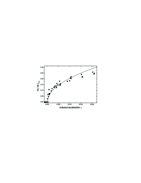
FIG. 5.: Sample S1: Bifurcation diagram for the maximum surface slope $\partial\eta/\partial x|_{{\rm max}}$. Symbols and parameters as in Fig. 3. The solid line is the asymptotics given by Eq. 16 for $\Omega\to\infty$.

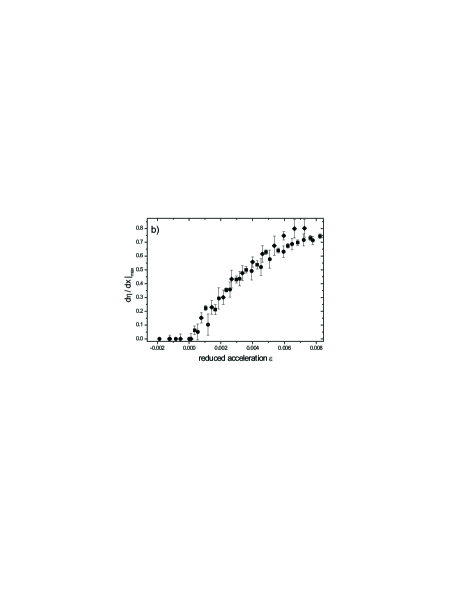
FIG. 6.: Sample S2 at $T=30^{\circ}{\rm C}$: Stationary wave slope $\partial\eta/\partial x|_{{\rm max}}$ at the drive frequencies $\Omega/2\pi=80{\rm Hz}$ (squares), $100{\rm Hz}$ (circles), $140{\rm Hz}$ (diamonds).

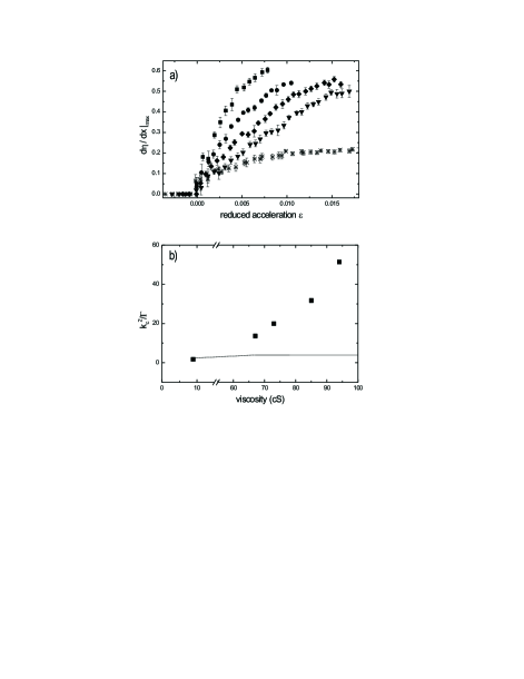
FIG. 7.: Sample $S2$ at different temperatures: (a) Bifurcation diagram $\partial\eta/\partial x|_{{\rm max}}$ at the drive frequency $\Omega/2\pi=80{\rm Hz}$. The viscosities are $\nu=94{\rm cS}$ (squares), $85{\rm cS}$ (circles), $73{\rm cS}$ (diamonds), $63{\rm cS}$ (down triangles), $8.35{\rm cS}$ (stars). (b) The coupling coefficient $1/\Gamma$ (scaled by $k_{c}^{2}$) as a function of the viscosity $\nu$. The symbols show the coefficient estimated by fitting the data of (a) for $\varepsilon<1\%$. The prediction of the perturbation analysis (solid line) becomes unreliable for viscosities above $\nu\simeq 50{\rm cS}$.

Sample	$T$	$\Omega/2\pi$	$\rho$	$\nu$	$\sigma$	$a_{c}$	$k_{c}$
	$[^{\circ}{\rm C}]$	$[{\rm Hz}]$	$[{\rm kg/m^{3}}]$	$[{\rm cS}]$	$[10^{-3}{\rm N/m}]$	$[{\rm g}]$	$[{\rm m^{-1}}]$
$S1$	30	60	934	8.35	20.1	1.23	1060
		80				1.91	1340
		120				3.85	1815
		160				6.2	2230
$S2$	30	80	955.4	94	20.55	15.1	1080
		100				21.7	1230
		140				37	1450
$S2$	35	80	950.9	85	20.2	14	1120
	45		941.9	73	19.5	12.5	1180
	50		937.5	67	19.15	11.7	1205

TABLE I.: Fluid specifications at different temperatures for the low (high) viscosity sample S1 (S2)

REFERENCES

- [1] for a review see: J. W. Miles and D. Henderson, Ann. Rev. Fluid Mech. 22, 143 (1990); H. W. Müller, R. Friedrich, and D. Papathanassiou, Theoretical and experimental studies of the Faraday instability, in: Lecture notes in Physics, ed. by F. Busse and S. C. Müller, Springer (1998).
- [2] S. T. Milner, J. Fluid Mech. 225, 81 (1990); K. Kumar and K. M. S. Bajaj, Phys. Rev. E 52, R4606 (1995); W. Zhang and J. Vinãls, Phys. Rev. E 53, 4283 (1996).
- [3] B. Christiansen and P. Alstrom, Phys. Rev. Lett. 68, 2157 (1992).
- [4] D. Binks and W. van de Water, Phys. Rev. Lett. 78, 4043 (1997).
- [5] A. Kudrolli and J. P. Gollub, Physica D 97, 133 (1997).
- [6] S. Douady, S. Fauve, and O. Thual, Europhys. Lett. 10, 309 (1989); A. B. Ezersky, D. A. Ermoshin, and S. V. Kiyashko, Phys. Rev. E 51, 4411 (1995).
- [7] E. Bosch and W. van de Water, Phys. Rev. Lett. 70, 3420 (1993); B. J. Gluckmann, P. Marcq, J. Bridger, and J. P. Gollub, Phys. Rev. Lett. 71, 2034 (1993); A. B. Ezersky, M. I. Rabinovich, V. P. Reutov and I. M. Starobinets, Sov. Phys. JETP 64, 1228 (1986).
- [8] C. L. Goodridge, W. T. Shi, and D. Lathrop, Phys. Rev. Lett. 76, 1824 (1996).
- [9] R. Ramshankar, D. Berlin, and J. .P. Gollub, Phys. Fluids A 2, 1955 (1990); E. Schröder, J. S. Andersen, M. T. Levinson, P. Alstrm and, W. I. Goldburg, Phys. Rev. Lett. 76, 4717 (1996).
- [10] K. Kumar and L. S. Tuckerman, J. Fluid Mech. 279, 49 (1994).
- [11] J. Bechhoefer, V. Ego, S. Manneville, and B. Johnson, J. Fluid Mech. 288, 325 (1995).
- [12] W. Zhang and J. Vinãls, J. Fluid. Mech. 336, 301 (1997).
- [13] W. S. Edwards and S. Fauve, J. Fluid Mech. 278, 123 (1994).
- [14] A. Kudrolli, B. Pier, and J. P. Gollub, Physica 123, 99(1998); H. Arbell and J. Fineberg, Phys. Rev. Lett. 81, 4384 (1998).
- [15] C. Wagner, H. W. Müller, and K. Knorr, Phys. Rev. E, 62, R33 (2000).
- [16] F. Raynal, S. Kumar, and S. Fauve, Eur. Phys. J. B 9, 175 (1999).
- [17] C. Wagner, H. W. Müller, and K. Knorr, Phys. Rev. Lett. 83, 308 (1999).
- [18] O. Lioubashevski, Y. Hamiel, A. Agnon, Z. Reches, and J. Fineberg, Phys. Rev. Lett. 83, 3190 (1999).
- [19] M. Silber and M. R. E. Proctor, Phys. Rev. Lett. 81, 2450 (1998); M. Silber and A. C. Skeldon, Phys. Rev. E 59, 5446 (1999).
- [20] S. S. Atatürk and K. B. Katsaros, J. Geophys. Res. 92, 5131 (1987).
- [21] M. Battezzati, J. Colloid and Interface Science 33, 24 (1970); M. L. Banner, I. S. F. Jones, and J. C. Trinder, J. Fluid Mech. 198, 321 (1989).
- [22] K. R. Nicolas, W. T. Lindenmuth, C. S. Weller, and D. G. Anthony, Exp. Fluids 23, 14 (1997).
- [23] R. Richter, Univ. Bayreuth, Germany, priv. comm.
- [24] M. Perlin, H. Lin, and C. Ting, J. Fluid Mech. 255, 597 (1993).
- [25] D. Dabiri, X. Zhang, and M. Gharib, Review of Scientific Instruments 67, 1858 (1996).
- [26] T. Roesgen, A. Lang, and M. Gharib, Exp. Fluids 25, 126, (1998).
- [27] S. Ciliberto and J. P. Gollub, Phys. Rev. Lett. 52, 922 (1984).
- [28] W. B. Wright, R. Budakian, and S. J. Putterman, Phys. Rev. Lett. 76, 4528 (1996).
- [29] S. Douady, J. Fluid Mechanics 221, 383 (1990).
- [30] J. C. Virnig, A. S. Berman, and P. R. Sethna, Transactions of the ASME 55, 220 (1988).
- [31] D. M. Henderson and J. W. Miles, J. Fluid Mech. 213, 95 (1989).
- [32] A. D. D. Craig and J. G. M. Armitage, Fluid Dyn. Res. 15, 129 (1995).
- [33] W. Zhang and J. Vinals, Physica D 116, 225 (1998).
- [34] W. W. Schultz, J. Vanden-Broeck, L. Jiang, and M. Perlin, J. Fluid Mech. 369, 253 (1998).
- [35] J. Wright, S. Yon, and C. Pozrikidis, J. Fluid Mech. 402, 1 (2000).
- [36] T. B. Benjamin and F. Ursell, Proc. R. Soc. London A 225, 505 (1954).
- [37] H. W. Müller, Phys. Rev. E 49, 1273 (1994).
- [38] D. Papathanassiou, Doktorarbeit, Universität des Saarlandes, 2000; D. Papathanassiou and H. W. Müller to be published.
- [39] F. H. Harlow and J. E. Welch, Phys. Fluids 8, 2182 (1965).
- [40] C. W. Hirt, B. D. Nichols, and N. C. Romero, Los Alamos Scientific Laboratory report LA-5852, April 1975.
- [41] W. Barten, M. Lücke, M. Kamps, Phys. Rev. Lett. 66, 2621 (1991); C. Jung, B. Huke, M. Lücke, Phys. Rev. Lett. 81, 3651 (1998).
- [42] D. B. Kothe, AIAA Journal 30, 2694 (1992).
- [43] M. Griebel, T. Dornseifer, and T. Neunhoeffer, Numerische Simulation in der Strömungsmechanik, Vieweg, Braunschweig (1995).