Resonantly Forced Inhomogeneous Reaction-Diffusion Systems

Abstract

The dynamics of spatiotemporal patterns in oscillatory reaction-diffusion systems subject to periodic forcing with a spatially random forcing amplitude field are investigated. Quenched disorder is studied using the resonantly forced complex Ginzburg-Landau equation in the 3:1 resonance regime. Front roughening and spontaneous nucleation of target patterns are observed and characterized. Time dependent spatially varying forcing fields are studied in the 3:1 forced FitzHugh-Nagumo system. The periodic variation of the spatially random forcing amplitude breaks the symmetry among the three quasi-homogeneous states of the system, making the three types of fronts separating phases inequivalent. The resulting inequality in the front velocities leads to the formation of “compound fronts” with velocities lying between those of the individual component fronts, and “pulses” which are analogous structures arising from the combination of three fronts. Spiral wave dynamics is studied in systems with compound fronts.

Spatially inhomogeneous reaction-diffusion equations may be used to model pattern formation and wave propagation in a variety of physical systems. We consider situations where the spatial inhomogeneity is externally imposed; for example, by inhomogeneous illumination of a light sensitive chemical reaction. The focus of the investigation is on resonantly forced oscillatory systems where the resonant forcing is a applied to the system in a spatially inhomogeneous fashion. Earlier experimental investigations of the light sensitive Belousov-Zhabotinsky under spatially homogeneous resonant forcing by an external light source revealed phase locked spatial patterns. We study wave propagation, pattern formation and spiral wave dynamics in oscillatory reaction-diffusion systems where the applied light field has a spatially random intensity pattern but varies periodically in time. The phenomena we observe include: roughening of fronts separating phase locked domains, nucleation of phase locked target patterns and compound fronts with distinct properties that give rise to unusual spiral wave dynamics. It should be possible to verify the phenomena described here by suitably designed experiments on light sensitive reacting systems.

I Introduction

Patterns in reaction-diffusion systems where the kinetics are spatiotemporally modulated can display a variety of phenomena that are not found in homogeneous systems.[1] Many reaction-diffusion processes of practical interest take place in inhomogeneous media or may be coupled to external processes that affect the kinetics in a non-uniform manner. A convenient experimental system for studying the effect of spatiotemporal modulations on pattern dynamics in spatially distributed systems is the ruthenium-catalyzed Belousov-Zhabotinsky (BZ) reaction. [2] This reaction is light-sensitive and thus the kinetics may be modulated by projecting a pattern of illumination of varying intensity onto the reaction medium.

Recent studies have made use of the light-sensitive BZ system to investigate wavefront propagation in systems with spatially disordered excitability. Kádár et al. studied stochastic resonance in a system with a periodically regenerated noise pattern.[3] Sendiña-Nadal et al. studied percolation and roughening of wavefronts in systems with quenched spatially disordered excitability; [4, 5] excitable spiral waves in the presence time-varying disorder were also studied.[6] The dynamics of reaction-diffusion waves in inhomogeneous excitable media is thought to be relevant to cardiac fibrillation since electrical waves may be disrupted by irregularities in the heart muscle medium.[7] Noise is thought to play a role in initiation and propagation of waves in neural tissue.[8] Earlier investigations into spatially inhomogeneous excitable systems include a study of a BZ medium containing catalyst-coated resin beads which served as nucleation sites for wavefronts [9], numerical simulations of a spatially-distributed network of coupled excitable elements which exhibited spontaneous wave initiation, stochastic resonance and fragmentation of wavefronts, [10, 11] and an excitable cellular automaton in which the refractory times of the elements were assigned randomly. [12] The effect of stochastic spatial inhomogeneities on other types of reaction-diffusion systems has been much less studied.

Periodically forced reaction-diffusion systems have also been investigated. Petrov et al. and Lin et al. subjected an oscillatory version of the light-sensitive BZ reaction to periodic spatially uniform illumination. [13, 14, 15] As the ratio of the forcing frequency to the natural frequency neared various resonances patterns were observed. In subsequent numerical studies the observed transition between labyrinthine and non-labyrinthine two-phased patterns at the 2:1 resonance was reproduced in the periodically forced Brusselator. [14, 15, 16] Belmonte et al. observed a transition from a stable spiral to turbulence in a BZ reaction when resonant forcing was applied. [17] Resonantly forced oscillatory systems have been investigated by numerical simulation as well as theoretically by Coullet and Emilsson, [18, 19] Coullet et al., [20] Elphick et al., [21, 22] and Chaté et al. [23] These systems exhibit a number of interesting pattern-forming phenomena.

Given the wide range of phenomena arising from spatial disorder in excitable systems and resonant forcing of oscillatory systems, one might expect that oscillatory systems with spatially inhomogeneous forcing have the potential to exhibit interesting new features. The research presented here explores qualitatively the phenomenology of such systems and characterizes some of the phenomena quantitatively. We restrict the focus of our study to systems in two spatial dimensions.

II Periodically Forced Oscillatory Systems

Consider an externally forced oscillatory reacting system described by the ordinary differential equation,

$$\frac{d{\mathbf{c}}(t)}{dt}={\mathbf{R}}({\mathbf{c}}(t);{\mathbf{a}},{\mathbf{b}}(t))\;,$$ (1)

where ${\mathbf{c}}(t)$ is a vector containing the concentrations of reagents. The reaction rates are described by the nonlinear vector function ${\mathbf{R}}$ which depends on a collection of parameters ${\mathbf{a}}$, such as rate constants and constant concentrations of pool chemicals, as well as parameters ${\mathbf{b}}(t)$ which comprise the periodic forcing and are of the form ${\mathbf{b}}(t)={\mbox{\boldmath$\eta$}}_{0}\Phi(\omega_{{\mathrm{f}}}t)$ with ${\mbox{\boldmath$\eta$}}_{0}$ the constant forcing amplitude and $\Phi$ a $2\pi$-periodic function giving the form of the forcing. As mentioned above, such forcing may be implemented by periodic illumination of the system if the reaction is light sensitive.

If ${\mathbf{b}}(t)={\mathbf{0}}$ we suppose the unforced reacting system has a stable limit cycle ${\mathbf{c}}_{0}(t)$ with period $T_{0}=2\pi/\omega_{0}$. In such a system there exists an infinite number of limit cycle solutions, ${\mathbf{c}}_{0}^{\prime}(t)={\mathbf{c}}_{0}(t+\Delta t)$ which differ from ${\mathbf{c}}_{0}(t)$ only by an arbitrary phase shift $2\pi\Delta t/T_{0}$. Limit cycle attractors are neutrally stable to phase perturbations corresponding to translations along the orbit. A system following a limit cycle will, in general, have undergone a phase shift when it returns to the limit cycle after experiencing a small perturbation.

These characteristics of the unforced oscillator may be contrasted with those of the forced oscillator. [24] If $\omega_{{\mathrm{f}}}/\omega_{0}$ is sufficiently close to an irreducible ratio of integers $n/m$, and if the forcing amplitude is sufficiently large, then the oscillations may become entrained to the external forcing and the system possesses $n$ stable limit cycle solutions of period $T=nT_{{\mathrm{f}}}=2n\pi/\omega_{{\mathrm{f}}}\approx mT_{0}$ which are mapped into each other under phase shifts $t\rightarrow t+kT/n$ for $k=0,1,2,\dots$. A system following one of these limit cycles will return to it with no phase shift after a small perturbation. This discrete, finite collection of limit cycles may be contrasted with the infinite and continuous collection of limit cycles in the unforced case. The entrained resonantly forced oscillator is a system with $n$ stable states, defined by the phase of the oscillations rather than by the system’s location in phase space.

The general form of an oscillatory reaction-diffusion system with spatially inhomogeneous periodic forcing is

$$\frac{\partial c({\mathbf{r}},t)}{\partial t}={\mathbf{R}}({\mathbf{c}}({\mathbf{r}},t);{\mathbf{a}},{\mathbf{b}}({\mathbf{r}},t))+{\mathbf{D}}\nabla^{2}{\mathbf{c}}({\mathbf{r}},t)\;,$$ (2)

where ${\mathbf{D}}$ is a diagonal matrix of diffusion coefficients. The parameters responsible for the periodic forcing ${\mathbf{b}}({\mathbf{r}},t)$ now depend on space as well as time and are of the form ${\mathbf{b}}({\mathbf{r}},t)={\mbox{\boldmath$\eta$}}({\mathbf{r}},t)\Phi(\omega_{{\mathrm{f}}}t)$. The random variable ${\mbox{\boldmath$\eta$}}({\mathbf{r}},t)$ accounts for the fact that the forcing amplitude may vary stochastically in space and time.

In a spatially distributed system with spatially uniform forcing, ${\mathbf{b}}({\mathbf{r}},t)={\mathbf{b}}(t)={\mbox{\boldmath$\eta$}}_{0}\Phi(\omega_{{\mathrm{f}}}t)$, the diffusive coupling and the stability of the $n$ limit cycles to phase perturbations leads to the formation of domains of the different phase locked states. At the domain walls separating the different phase locked states the phase of the oscillations shifts by an amount determined by the character of the phase locking. In two dimensions, $n$-armed spiral waves may form, given suitable initial conditions, if the domain walls have non-zero velocity. The core of the spiral wave is a phase singularity at which all $n$ states meet and around which the phase advances by $2m\pi$. The rotation of these phase locked spirals is a result of the propagation of the phase dislocations comprising the domain walls; thus, they rotate much more slowly than spiral waves in the unforced system, where the spiral rotation frequency is equal to the frequency of the local oscillations.

In this article we investigate systems subjected to periodic forcing with a stochastic component, either quenched disorder, ${\mbox{\boldmath$\eta$}}({\mathbf{r}},t)={\mbox{\boldmath$\eta$}}({\mathbf{r}})$, where the periodically applied perturbation has a random distribution in space which does not change in the course of the evolution, and systems with dynamic disorder, ${\mbox{\boldmath$\eta$}}({\mathbf{r}},t)$, where the spatial distribution of the perturbation may change with time. The reduction of a resonantly forced oscillatory system to a complex Ginzburg-Landau (CGL) equation by Gamabaudo [25] and by Elphick et al [26] may be simply extended to systems with quenched disorder and consequently we have employed the CGL equations in our studies of this case. For time-varying disorder, one must reconsider the derivation of the appropriate CGL equation because of the presence of another time scale associated with the noise process; hence, we have chosen instead to study the FitzHugh-Nagumo system as a typical example of an oscillatory reaction-diffusion system.

In such cases a new length, $\ell_{s}$, related to the spatial correlation range of the noise distribution enters the problem. The behavior of the system will depend on the magnitude of this length relative to that of other important lengths in the system, such as the diffusion length $\ell_{D}$ and the typical width of a domain wall or propagating front, $w_{d}$. If $\ell_{s}$ is sufficiently small compared to both of these lengths the system will appear effectively homogeneous and behave as if it were subject to periodic forcing with amplitude determined by the spatial average $\overline{{\mbox{\boldmath$\eta$}}}$ of ${\mbox{\boldmath$\eta$}}({\mathbf{r}})$. If $\ell_{s}$ is very large compared to these lengths then the system dynamics may be simply represented in terms of the dynamics of a collection of uniformly forced patches. The interesting regime is when these length scales are comparable and our studies focus on these cases.

III Forced CGL with quenched disorder

In the vicinity of the Hopf bifurcation point a periodically forced oscillatory reaction-diffusion system may be reduced to its normal form, the forced complex Ginzburg-Landau equation (FCGL) [25, 26]. This reduction is valid provided the system is near an $n:m$ resonance, where $n=1,2,3,4$. Such a reduction may also be carried out for the case of quenched disorder, ${\mbox{\boldmath$\eta$}}({\mathbf{r}},t)={\mbox{\boldmath$\eta$}}({\mathbf{r}})$, and the FCGL takes the form,

$$\frac{\partial A({\mathbf{r}},t)}{\partial t} = (\mu+i\nu)A-(1+i\beta)|A|^{2}A$$ (4)

$$\qquad\qquad+\;\gamma({\mathbf{r}})\bar{A}^{n-1}+(1+i\alpha)\nabla^{2}A\;,$$

where $\gamma({\mathbf{r}})$ accounts for the spatial variation of the forcing amplitude. The complex amplitude $A({\mathbf{r}},t)$ describes slow modulations in the frequency and amplitude of oscillations of the original system in Poincaré planes taken at the forcing period; $\bar{A}$ denotes the complex conjugate of $A$. Equation (4) with $\gamma({\mathbf{r}})\equiv\gamma_{0}$, a constant, has been used as a model for an oscillatory reaction-diffusion system with spatially uniform resonant forcing. [18, 19, 20, 21, 22, 23]

Consider the normal form of a single resonantly forced oscillator obtained by omitting the diffusion terms and spatial dependence in $\gamma({\mathbf{r}})$,

$$\frac{dA(t)}{dt}=(\mu+i\nu)A-(1+i\beta)|A|^{2}A+\gamma\bar{A}^{n-1}\;.$$ (5)

For Eq. (5) a critical $\gamma_{c}$ exists such that for $\gamma<\gamma_{c}$ the equation exhibits a stable limit cycle solution, while for $\gamma\geq\gamma_{c}$ there are $n$ stable fixed points. These correspond to the $n$ stable limit cycle solutions of the original system and can be mapped into each other by phase shifts $A\rightarrow Ae^{i2\pi/n}$. More specifically, the fixed points can be found from the stationary solutions of Eq. (5) by expressing the complex amplitude in the form $A=Re^{i\phi}$. The modulus, $R_{0}$, of the non-zero fixed points of Eq. (5) depends on $\gamma$ according to

$$\gamma^{2}=\frac{(R_{0}^{2}-\mu)^{2}+(\nu-\beta R_{0}^{2})^{2}}{R_{0}^{2(n-2)}}\;.$$ (6)

For some values of $n$ and $\gamma$ Eq. (6) permits multiple $R_{0}$ values, some of which may correspond to unstable fixed points. Figure 1 shows a $\gamma$ vs. $R_{0}$ curve for $n=3$; the upper branch corresponds to the stable fixed points while the lower branch describes the nonzero unstable fixed points. The parameter values used to construct this figure are $\mu=1$, $\nu=0$, $|\beta|=0.6$. Note the presence of a critical forcing amplitude $\gamma_{c}\approx 0.58$ below which phase locking does not occur. For $n=3$, Eq. (6) gives $\gamma_{c}=\bigl{[}2\bigl{(}(1+\beta^{2})(\mu^{2}+\nu^{2})\bigr{)}^{\leavevmode\kern 0.70004pt\raise 1.50694pt\hbox{\sevenrm1}\kern-0.70004pt/\kern-1.04996pt\lower 0.75346pt\hbox{\sevenrm2}}-2(\mu+\beta\nu)\bigr{]}^{\leavevmode\kern 0.70004pt\raise 1.50694pt\hbox{\sevenrm1}\kern-0.70004pt/\kern-1.04996pt\lower 0.75346pt\hbox{\sevenrm2}}$.

FIG. 1.: The modulus, $R_{0}$, of the stable (solid line) and unstable (dashed line) fixed points of Eq. 5 as a function of forcing intensity $\gamma$. The parameter values are $n=3$, $|\beta|=0.6$, $\mu=1$, $\nu=0$. The three arrows indicate the values $\gamma=0.0$, $0.6$ and $1.0$, which were used in simulations described in Section III. The vertical dotted line is located at $\gamma_{c}$, the critical value for phase locking.

As an example of quenched disorder in resonantly forced oscillatory systems the $\gamma({\mathbf{r}})$ fields were taken to be dichotomous random variables. Two values for the forcing amplitude, $\gamma_{1}$ and $\gamma_{2}$, were chosen. The two-dimensional system was partitioned into square cells and the value of $\gamma({\mathbf{r}})$ in each cell was chosen to be either $\gamma_{1}$, with probability $p$, or $\gamma_{2}$ with probability $q=1-p$. More precisely, if the noise cells have dimension $s\times s$ and the system’s dimensions are $W\times L=sN_{W}\times sN_{L}$ then

$$\gamma({\mathbf{r}})=\sum_{i=1}^{N_{W}}\sum_{j=1}^{N_{L}}\xi_{ij}\Theta_{ij}({\mathbf{r}})\;,$$ (7)

where

$$\xi_{ij}=\left\{\begin{array}[]{c@{\quad\mbox{with probability} \quad}l}\gamma_{1}&p\\ \gamma_{2}&q=1-p\;,\end{array}\right.$$ (8)

and

$$\Theta_{ij}({\mathbf{r}}) = \Theta_{ij}(x,y)$$ (9)

$$= \theta(x-(i-1)s)\;\theta(is-x)$$ (11)

$$\quad\times\;\theta(y-(j-1)s)\;\theta(js-y)\;,$$

where $\theta$ is the Heaviside function and $(ij)$ are the discrete coordinates of a noise cell. For quenched disorder this distribution is fixed for all time. The cell size, the values of $\gamma_{1}$ and $\gamma_{2}$ and the seeding probabilities $p$ and $q$ are the relevant parameters to consider. The probabilities $p$ and $q$ were typically, but not necessarily, independent of position; exceptions will be noted as they occur. This $\gamma({\mathbf{r}})$ field has the mean value $\bar{\gamma}=p\gamma_{1}+q\gamma_{2}$, and spatial autocorrelation

$$C({\mathbf{r}^{\prime}}) = \frac{\left<\delta\gamma({\mathbf{r}^{\prime}}+{\mathbf{r}^{\prime\prime}})\;\delta\gamma({\mathbf{r}^{\prime\prime}})\right>}{\left<\delta\gamma({\mathbf{r}^{\prime\prime}})\;\delta\gamma({\mathbf{r}^{\prime\prime}})\right>}\;,$$ (12)

$$= \left\{\begin{array}[]{c@{\quad}c}\left(1-\frac{|x^{\prime}|}{s}\right)\left(1-\frac{|y^{\prime}|}{s}\right)&{\mathrm{i}f}\;|x^{\prime}|\leq s\;{\mathrm{a}nd}\;|y^{\prime}|\leq s\\ {}\hfil&{}\hfil\\ 0&{\mathrm{o}therwise}\end{array}\right.$$ (16)

where $\delta\gamma({\mathbf{r}})=\gamma({\mathbf{r}})-\bar{\gamma}$, ${\mathbf{r}^{\prime}}=(x^{\prime},y^{\prime})$ and the average $\langle\cdot\rangle$ is taken over all ${\mathbf{r}^{\prime\prime}}$.

The studies described in this paper investigate patterns at the 3:1 resonance. For such systems there are two interesting cases for resonant forcing with a dichotomous $\gamma({\mathbf{r}})$ field. In the first case both $\gamma_{1}$ and $\gamma_{2}$ lie above the phase locking threshold, $\gamma_{c}$, so that all regions of the medium are entrained to the forcing. In the second case only one of $\gamma_{1}$ or $\gamma_{2}$ lies above the threshold and the medium consists of a mixture of entrained and non-entrained regions. In the simulations described below, including those in Sec. IV, numerical integration was performed using explicit forward differencing and a second-order discrete Laplacian.

A All sites phase locked; front roughening

When both $\gamma_{1}$ and $\gamma_{2}$ lie above the phase locking threshold $\gamma_{c}$ then all regions of the medium are tristable. The system possesses three quasi-homogeneous stationary states in which the complex amplitude fluctuates about an average value. Domain walls separating these phase locked states are in general non-stationary in the $3:1$ resonant regime since all three phases are inequivalent, although their velocity may pass through zero as parameters are tuned. Initially planar fronts in these inhomogeneously forced systems roughen as they propagate. Figure 2 shows an example of a rough interface separating two of the three phases.

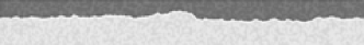
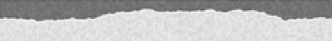
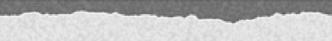
FIG. 2.: Interfaces of the 3:1 inhomogeneously forced CGL from a single realization in a moving frame, at three well separated times. The phase, $\phi$ of the complex amplitude $A=Re^{i\phi}$ is shown, using a gray-scale in which $\phi=-\pi=+\pi$ is white and $\phi=0$ is black. The system size, $L\times W$ is $800\times 100$. The noise grain size is $s\times s=W/25\times W/25$. Other parameters are given in the text. Boundary conditions are periodic along $x$ and no-flux along $y$.

Front roughening is also observed if $\gamma_{1}<\gamma_{c}<\gamma_{2}$, (i.e. when the medium consists of a mixture of entrained and non-entrained regions) but is difficult to study because spontaneously nucleated patterns interfere with propagating fronts. This case will be examined below.

The propagating fronts in this system experience local velocity fluctuations arising from spatial variations in the $\gamma({\mathbf{r}})$ field. Diffusion will tend to eliminate front roughness generated by random fluctuations in the $\gamma({\mathbf{r}})$ field; consequently, the front dynamics should obey the Kardar-Parisi-Zhang (KPZ) equation, [27]

$$\frac{\partial h(x,t)}{\partial t}=\bar{v}+D\frac{\partial^{2}h}{\partial x^{2}}+\frac{\lambda}{2}\left(\frac{\partial h}{\partial x}\right)^{2}+\zeta(x,t)\;,$$ (17)

where $h(x,t)$ is the front position, $\bar{v}$ is the average front velocity, $D$ and $\lambda$ are phenomenological coefficients and $\zeta(x,t)$ is Gaussian white noise with zero mean and correlation $\langle\zeta(x^{\prime},t^{\prime})\,\zeta(x^{\prime\prime},t^{\prime\prime})\rangle=2\Gamma\,\delta(x^{\prime}-x^{\prime\prime})\,\delta(t^{\prime}-t^{\prime\prime})$. In such a circumstance the interface width $w(t)=(L^{-1}\sum_{i}(h(x_{i},t)-\bar{h}(t))^{2}\;\Delta x)^{\leavevmode\kern 0.70004pt\raise 1.50694pt\hbox{\sevenrm1}\kern-0.70004pt/\kern-1.04996pt\lower 0.75346pt\hbox{\sevenrm2}}$ increases with time as $w(t)\sim t^{\hat{\beta}}$ for short times; the average width of a saturated front, $w_{{\mathrm{s}}}$, scales with system size as $w_{{\mathrm{s}}}\sim L^{\hat{\alpha}}$, where $\hat{\alpha}=1/2$ and $\hat{\beta}=1/3$.

We have verified these KPZ scaling properties for a FCGL system with parameter values ($\alpha=1$, $\beta=0.6$, $\mu+i\nu=1$) and the forcing field parameters ($\gamma_{1}=0.60$, $\gamma_{2}=1$, $p=0.50$) for which the critical forcing amplitude is $\gamma_{c}\approx 0.58$ (cf. Fig. 1). The front properties were measured in a frame moving with the front. The system dimensions were $W=100$ and $L=100$, $200$, $400$ and $800$. The noise grain size was $s\times s=W/25\times W/25$. The boundary conditions were periodic along the boundaries perpendicular to the front, and no-flux along the boundaries perpendicular to the direction of front motion.

The saturated front width $w_{{\mathrm{s}}}$ was found to scale with system size as $w_{{\mathrm{s}}}\sim L^{1/2}$. Plotting $\langle w(t)\rangle/L^{\hat{\alpha}}$ against $t/L^{\hat{\alpha}/\hat{\beta}}$ collapses the $\langle w(t)\rangle$ versus $t$ data for four different $L$ onto a single curve when the KPZ values $\hat{\alpha}=1/2$, $\hat{\beta}=1/3$ are used, as shown in Fig. 3. Here $\langle\cdot\rangle$ denotes an average over realizations.

The width temporal autocorrelation function

$$C_{w}(t)=\frac{\langle\delta w(t+t^{\prime})\;\delta w(t^{\prime})\rangle}{\langle\delta w(t^{\prime})\;\delta w(t^{\prime})\rangle}\;,$$ (18)

was calculated for fronts in the saturated regime at four system sizes $L=100$, $200$, $400$ and $800$. Here $\langle\cdot\rangle$ represents a time average within the saturated regime. Temporal correlations were found to decay to zero, with the rate of decay decreasing as system size increases (Fig. 4). This is expected, since the larger system size allows larger fluctuations in the front profile which require longer times to form and decay.

FIG. 3.: Early time $\langle w(t)\rangle$ vs. $t$ curves for initially planar fronts in the $3:1$ inhomogenously forced CGL rescaled according to the KPZ scaling exponents. Curves are shown for system sizes $L=100$ (dotted line), $200$ (short dashes), $400$ (long dashes) and $800$ (solid line). Each curve results from the average over 80 realizations of the stochastic dynamics.

FIG. 4.: The width temporal autocorrelation function for saturated interfaces in the 3:1 inhomogenously forced CGL for system sizes $L=100$ (dotted line), $200$ (short dashes), $400$ (long dashes) and $800$ (solid line).

To investigate the presence of spatial correlations in saturated front profiles, the height spatial autocorrelation function

$$C_{h}(x)=\left<\frac{\langle\delta h(x+x^{\prime})\;\delta h(x^{\prime})\rangle}{\langle\delta h(x^{\prime})\;\delta h(x^{\prime})\rangle}\right>\;,$$ (19)

was calculated for the various system sizes. In Eq. (19) the inner $\langle\cdot\rangle$ refer to averaging over $x^{\prime}$ in a single front profile and the outer $\langle\cdot\rangle$ refers to averaging over different saturated front profiles. Results for $L=100$ and $L=800$ are shown (Fig. 5).

In the case of a front free of spatial structure, i.e. a periodic random walk that returns to its initial position in $N$ steps, the height spatial autocorrelation function is of the form $C_{h}^{R}(x)=1-(2{\mathcal{D}}/L)x(L-x)$, where ${\mathcal{D}}$ is a phenomenological diffusion coefficient. [28] The deviations of the fit of the numerically determined $C_{h}(x)$ from a quadratic function indicate the existence of spatial correlations.

FIG. 5.: The height spatial autocorrelation functions for saturated fronts in systems of size $L=100$ (solid line) and $L=800$ (long dashes). The best fit quadratic functions are shown for $L=100$ (dotted line) and $L=800$ (short dashes).

B A medium with phase locked and oscillatory sites; spontaneous nucleation of target patterns

When $\gamma_{1}<\gamma_{c}$ and $\gamma_{2}>\gamma_{c}$, the system consists of a mixture of tristable regions and oscillatory regions. If the density of oscillatory sites, $p$, is low the diffusive coupling maintains the value of $A$ within the oscillatory regions near that in the adjacent tristable regions. The medium behaves essentially like a tristable medium and supports three quasi-homogeneous stable stationary states, travelling kink-like domain walls and three-armed spiral waves. The oscillatory sites provide a spatial inhomogeneity that leads to roughening of domain walls and to fluctuations of the concentrations within domains.

With increasing $p$, target patterns are observed (Fig. 6). They consist of concentric, approximately circular domain walls moving outwards from a central region (a “pacemaker”) where they are initiated periodically. Within each ring of the target the concentration is quasi-homogeneous. Note that all images in Fig. 6 are from realizations with identical parameters, however a range of wavelengths is observed.

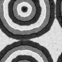
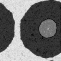
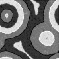
FIG. 6.: Target patterns generated in the 3:1 forced CGL from spatially homogeneous initial conditions. The phase, $\phi$ of the complex amplitude $A=Re^{i\phi}$ is shown, using a gray-scale in which $\phi=-\pi=+\pi$ is white and $\phi=0$ is black. Forcing field parameters are ($\gamma_{1}=0$, $\gamma_{2}=1$, $p=0.30$). Other parameters are ($\mu+i\nu=1$, $\alpha=1$, $\beta=0.6$), for which $\gamma_{c}\approx 0.58$. The system size is $L\times L=200\times 200$, the noise grain size is $s\times s=L/200\times L/200$. Boundary conditions are periodic.

The probability of a realization possessing a target pattern was measured as a function of $p$ and system size (Fig. 7). It was found to approach zero for low $p$, one for high $p$, and to increase rapidly around some critical $p_{c}$. Figure 7 shows results for the parameter values ($\mu+i\nu=1$, $\alpha=1$, $\beta=-0.6$) and forcing field parameters ($\gamma_{1}=0$, $\gamma_{2}=1$); qualitatively similar results were also obtained for ($\mu+i\nu=1$, $\alpha=1$, $\beta=0.6$, $\gamma_{1}=0$, $\gamma_{2}=1$) and ($\mu+i\nu=0$, $\alpha=2$, $\beta=-0.82$, $\gamma_{1}=0$, $\gamma_{2}=1$). For larger system sizes, the probability of occurrence of a target pattern is higher, consistent with a fixed probability per unit area of the medium nucleating a target pattern.

FIG. 7.: The fraction of realizations in which one or more pacemakers occurred as a function of $p$, the density of oscillatory ($\gamma=\gamma_{1}=0$) sites. Results from numerical simulations with noise grain size $s\times s=0.5\times 0.5$ are shown for system sizes $50\times 50$ ($\vartriangle$) and $100\times 100$ ($\blacktriangledown$). The curves predicted by the model described in the text (Eqs. (23)-(27)) with the parameter values $\gamma^{*}=0.65$ and ${\mathcal{N}}_{p}=180$ are shown for these same system sizes as solid and dashed lines, respectively.

The occurrence of target patterns may be explained by supposing that diffusion provides a mechanism for averaging $\gamma({\mathbf{r}})$ over some length scale, and that regions of the medium behave qualitatively like a uniform medium with the same local average $\bar{\gamma}({\mathbf{r}})$. Thus the medium is locally tristable for a high $\bar{\gamma}({\mathbf{r}})$, but if $\bar{\gamma}({\mathbf{r}})$ is sufficiently low it will be oscillatory. As the density of oscillatory sites increases, it becomes increasingly likely that there will exist regions with a local $\gamma$ sufficiently low to exhibit oscillatory dynamics.

We can determine a profile of the average $\gamma$ field around the average pacemaker. We define $\bar{\gamma}_{{\mathrm{p}}}$ as the average value of $\gamma$ a distance $R$ from the center of a pacemaker. This is given by

$$\bar{\gamma}_{{\mathrm{p}}}(R)=\frac{1}{2\pi R}\frac{d}{dR}\pi R^{2}\bar{\gamma}_{{\mathrm{d}}}(R)\;,$$ (20)

where

$$\bar{\gamma}_{{\mathrm{d}}}(R)=\left\langle\frac{1}{\pi R^{2}}\int_{|{\mathbf{r}}-{\mathbf{r}}_{0}|\leq R}\gamma({\mathbf{r}})\,d{\mathbf{r}}\right\rangle\;,$$ (21)

is the average value of $\gamma$ over a disk of radius $R$, averaged over all pacemakers in all realizations with a given set of parameters. In practice, $\bar{\gamma}_{{\mathrm{p}}}$ is calculated as the discrete derivative

$$\bar{\gamma}_{{\mathrm{p}}}(R)=\frac{\pi(R+\Delta R)^{2}\bar{\gamma}_{{\mathrm{d}}}(R+\Delta R)-\pi R^{2}\bar{\gamma}_{{\mathrm{d}}}(R)}{\pi(R+\Delta R)^{2}-\pi R^{2}}\;.$$ (22)

Figure 8 shows $\bar{\gamma}_{{\mathrm{p}}}$ and $\bar{\gamma}_{{\mathrm{d}}}$ for $p=0.30$, system size $L\times L=100\times 100$, noise grain size $s\times s=L/200\times L/200$, and other parameter values equal to those used to measure the nucleation probability curves shown in Fig. 7. Qualitatively similar plots, in which $\bar{\gamma}_{{\mathrm{p}}}$ and $\bar{\gamma}_{{\mathrm{d}}}$ increase from a low value at $R=0$ to the mean-field value, $\bar{\gamma}$, at high $R$ were observed for other values of $p$. Also shown in Fig. 8 are $\bar{\gamma}_{{\mathrm{p}}}$ calculated from the neighborhoods of points chosen randomly from the realizations rather than from points centered on pacemakers, and the mean-field value, $\bar{\gamma}$.

FIG. 8.: The solid curve shows $\bar{\gamma}_{{\mathrm{p}}}(R)$; the long-dashed curve is $\bar{\gamma}_{{\mathrm{d}}}$. Averages are taken over 20 realizations. The short-dashed curve shows $\bar{\gamma}_{{\mathrm{p}}}$ calculated around points chosen randomly from the realizations. A horizontal line indicates $\bar{\gamma}=0.70$. The values $\gamma^{*}=0.65$, ${\mathcal{R}}=3.8$, calculated using the pacemaker model, are also shown.

Consider the following simple model of pacemaker formation. We divide the system into ${\mathcal{N}}$ “sites” of size $\Delta x\times\Delta x$ such that the value of $\gamma$ is constant over a site; i.e., the sites may be noise domains or subdivisions of noise domains. We assume that, on average, pacemakers have a radius of ${\mathcal{R}}$ and contain ${\mathcal{N}}_{p}=\pi({\mathcal{R}}/{\Delta x})^{2}$ sites. Thus we divide the system into ${\mathcal{N}}/{\mathcal{N}}_{p}$ independent domains which are potential pacemakers. We assume that such a domain is a pacemaker if the average value of $\gamma$ within it is less than some threshold for oscillatory behavior, $\gamma^{*}$. If $N_{1}$ is the number of sites on which $\gamma=\gamma_{1}$ and $N_{2}={\mathcal{N}}_{p}-N_{1}$ is the number of $\gamma_{2}$ sites, then the potential pacemaker is a pacemaker when

$$\frac{\gamma_{1}N_{1}+\gamma_{2}N_{2}}{{\mathcal{N}}_{p}}=\frac{\gamma_{1}N_{1}+\gamma_{2}({\mathcal{N}}_{p}-N_{2})}{{\mathcal{N}}_{p}}\leq{\gamma^{*}}\;,$$ (23)

that is, when

$$N_{1}\geq\frac{\gamma_{2}-\gamma^{*}}{\gamma_{2}-\gamma_{1}}{\mathcal{N}}_{p}\;.$$ (24)

Defining

$$N^{*}=\left\lceil\frac{\gamma_{2}-\gamma^{*}}{\gamma_{2}-\gamma_{1}}{\mathcal{N}}_{p}\right\rceil\;,$$ (25)

the probability that a domain is a pacemaker is

$${\mathcal{P}}=\sum_{k=N^{*}}^{{\mathcal{N}}_{p}}{{\mathcal{N}}_{p}\atopwithdelims( )k}p^{k}q^{{\mathcal{N}}_{p}-k}\;,$$ (26)

and it is not a pacemaker with probability ${\mathcal{Q}}=1-{\mathcal{P}}$. The probability that the entire system possesses no pacemakers is ${\mathcal{Q}}^{{\mathcal{N}}/{\mathcal{N}}_{p}}$ and it possesses one or more pacemakers with probability

$$P({\mathcal{N}},p)=1-{\mathcal{Q}}^{{\mathcal{N}}/{\mathcal{N}}_{p}}\;.$$ (27)

The parameters ${\mathcal{N}}_{p}$ and $\gamma^{*}$ uniquely determine the $P({\mathcal{N}},p)$ surface. The values giving the best fit to the experimental data were $\gamma^{*}=0.65$ and ${\mathcal{N}}_{p}=180$ which implies ${\mathcal{R}}\approx 3.8$. These values are compared with the numerically determined $\bar{\gamma}_{{\mathrm{d}}}(R)$ curve in Fig. 8. The simple model predicts that the average pacemaker should have $\bar{\gamma}_{{\mathrm{d}}}({\mathcal{R}})=\gamma^{*}$; the point $({\mathcal{R}},\gamma^{*})$ lies close to, but not on, the $\bar{\gamma}_{{\mathrm{d}}}$ curve.

In order to provide further insight into the criteria necessary for a region to act as a pacemaker, a series of studies was carried out in which the $\gamma$ field consisted of a disk of radius $R$ sites with a density $p_{{\mathrm{i}n}}$ of oscillatory sites. This disk was embedded in a field with density of oscillatory sites $p_{{\mathrm{o}ut}}$. In all cases $p_{{\mathrm{i}n}}$ was greater than $p_{{\mathrm{o}ut}}$, so that the disk could act as a pacemaker. Multiple realizations of the evolution were simulated at various values of $R$, $p_{{\mathrm{i}n}}$ and $p_{{\mathrm{o}ut}}$, and the fraction of realizations Pr(br) in which the central disk emitted target waves into the surrounding medium (i.e. in which “breakout” occurred) was measured.

Figure 9 shows Pr(br) as a function of $R$ and $p_{{\mathrm{i}n}}$ for $p_{{\mathrm{o}ut}}=0.10$. As one would expect, Pr(br) increases as $R$ increases and decreases as $p_{{\mathrm{i}n}}$ decreases, with the exception that at $p_{{\mathrm{i}n}}=1$ the probability of breakout increases with $R$ until $R=3$ and then decreases for $3<R<5$, after which it increases. (cf. Figs. 9 and 10). For $p_{{\mathrm{i}n}}=0.95$, when there is a small fraction of tristable sites in the inner disk, the magnitude of the decrease is substantially reduced (cf. Fig. 10). Apart from the anomalous region at low $p_{{\mathrm{i}n}}$ the trends that Pr(br) increases with increasing $R$ and decreases with decreasing $p_{{\mathrm{i}n}}$ are consistent with the notion that pacemakers form when the local density of oscillatory sites is high. The behavior for $p_{{\mathrm{o}ut}}=0.15$ was qualitatively similar.

FIG. 9.: The fraction of realizations in which target waves were emitted from the central disk region. Parameter values apart from $p$ are as in Figs. 7 and 8; the noise grain size is $0.5\times 0.5$. Here $p_{{\mathrm{o}ut}}=0.10$.

FIG. 10.: Fraction of realizations in which target waves were emitted from the central disk region as a function of $R$, for $p_{{\mathrm{o}ut}}=0.1$ and $p_{{\mathrm{i}n}}=1.0$ (solid line) and $p_{{\mathrm{i}n}}=0.95$ (dashed line).

The anomalous decrease between $R=3$ and $R=5$ is possibly related to the fact that the anomalous behavior begins when $R\approx\ell_{D}$, where $\ell_{D}$ is the diffusion length of the unforced system ($\gamma({\mathbf{r}})\equiv\gamma_{1}=0$). We find the diffusion length $\ell_{D}=\sqrt{D\tau}\approx 3.24$ by taking the diffusion coefficient $D$ to be unity, and the characteristic time $\tau$ to be equal to $2\pi/\beta\mu$, the period of homogeneous oscillations in the unforced system for the parameters $\beta=-0.6$, $\mu=1$ used in these studies. Parts of the system separated by a length greater than $\ell_{D}$ evolve independently over time intervals less than $\tau$. For large $R$ one observes that pacemaker nucleation occurs locally on the boundary of the disk. As the disk perimeter increases with $R$ so does the probability of forming a local pacemaker on the disk boundary.

In addition to the target patterns discussed above, one may also observe spiral waves if the initial conditions contain a phase defect. An example of such a spiral is shown in Fig. 11. It was formed in a realization with $\bar{\gamma}=0.50<\gamma_{c}$, hence the medium may be thought of as oscillatory, exhibiting three-fold symmetric relaxational local dynamics, rather than as tristable.

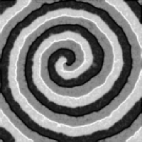
FIG. 11.: Spiral wave in the 3:1 inhomogeneously forced CGL. The phase, $\phi$ of the complex amplitude $A=Re^{i\phi}$ is shown, using a gray-scale in which $\phi=-\pi=+\pi$ is white and $\phi=0$ is black. Parameters: $\alpha=1$, $\beta=-0.6$, $\mu+i\nu=1$, $\gamma_{1}=0$, $\gamma_{2}=1$, $p=0.50$, $L=100$, $s=L/200$, no-flux boundary conditions.

IV Systems with time-varying spatial disorder

We now consider situations where the spatial distribution of forcing amplitudes varies in time. For this purpose we examine the behavior of the spatially distributed FitzHugh-Nagumo (FHN) system

$$\frac{\partial u({\mathbf{r}},t)}{\partial t} = u-u^{3}-v+D_{u}\nabla^{2}u$$ (28)

$$\frac{\partial v({\mathbf{r}},t)}{\partial t} = \epsilon\bigl{(}u-av+b({\mathbf{r}},t)\bigr{)}+D_{v}\nabla^{2}v\;,$$ (29)

subject to such time-varying noise distributions. Here $u({\mathbf{r}},t)$ and $v({\mathbf{r}},t)$ are the “concentrations”, $a$ and $\epsilon$ are constant parameters, $D_{u}$ and $D_{v}$ are the diffusion coefficients and $b({\mathbf{r}},t)$ is a forcing function of the form $\eta({\mathbf{r}},t)\cos\omega_{{\mathrm{f}}}t$ with the forcing amplitude $\eta({\mathbf{r}},t)$ a random variable. We have chosen this form to make explicit the periodic component of the external forcing whose amplitude is a periodically or randomly updated spatial random variable. In the applications described below $\eta({\mathbf{r}},t)$ is updated on a time scale that is some multiple of the forcing period.

Before considering Eq. (29) we discuss the associated system of ordinary differential equations

$$\frac{d}{dt}u(t) = u-u^{3}-v$$ (30)

$$\frac{d}{dt}v(t) = \epsilon(u-av+b)\;,$$ (31)

in which $b$ is a constant. If $0<a<1$ the system possesses a single fixed point. If, in addition, $b=0$, then the fixed point is unstable and the system exhibits a stable limit cycle whenever $a\epsilon<1$. In this article we consider only systems with $0<a<1$ and $a\epsilon<1$. Figure 12 shows the limit cycle for a system with $a=0.3$, $\epsilon=0.1$ and $b=0$. Also shown are the cubic $u$-nullcline and the linear $v$-nullcline for different $b$ values. The effect of varying $b$ is to shift the $v$-nullcline relative to the $u$-nullcline. As $|b|$ increases from zero the limit cycle contracts in the phase plane, eventually collapsing to a stable fixed point at a Hopf bifurcation that occurs when $|b|=b_{H}=\bigl{(}1-(2a+a^{2}\epsilon)/3\bigr{)}\bigl{(}(1-a\epsilon)/3\bigr{)}^{\leavevmode\kern 0.70004pt\raise 1.50694pt\hbox{\sevenrm1}\kern-0.70004pt/\kern-1.04996pt\lower 0.75346pt\hbox{\sevenrm2}}$. For $|b|>b_{H}$ the system exhibits excitable kinetics. Figure 12 shows $v$-nullclines corresponding to $b=\pm 0.46$, which lies just inside the excitable regime.

FIG. 12.: The nullclines and limit cycle of the FHN system (Eq. 31), with $\alpha=0.3$. The cubic $u$ nullcline and linear $v$ nullcline corresponding to $b=0$ are shown as solid lines. The dashed lines are the $v$ nullclines for $b=\pm 0.46$, for which the system is excitable. The limit cycle for $b=0$, $\epsilon=0.1$ is also shown.

Given this background, we consider the dynamics of Eq. (29) as an example of an oscillatory reaction-diffusion system with periodic forcing. The forcing amplitude field $\eta({\mathbf{r}},t)$ was similar to the $\gamma({\mathbf{r}})$ fields used in the quenched disorder studies described earlier in that the system was divided into squares which were randomly assigned one of the two forcing intensities $\eta_{1}$ and $\eta_{2}$. This disordered forcing amplitude field was periodically updated, with the new values of the amplitude in the spatial distribution drawn from the same dichotomous distribution of amplitudes. The updating period was taken to be $nT_{{\mathrm{f}}}$ time units, which is the period of the corresponding $n:m$ entrained ordinary differential equation. (The investigations described here consider only the case where the updating is on resonance, i.e. where the interval between updates is $nT_{{\mathrm{f}}}$. We shall not consider the case of periodic updating where the updating is off-resonance.)

The $nT_{{\mathrm{f}}}$-periodic updating of the forcing amplitude field may have a phase offset relative to the $T_{{\mathrm{f}}}$-periodic forcing $\cos\omega_{{\mathrm{f}}}t$. We describe this offset with the parameter $\sigma$ which ranges from 0 to 1 and specifies the phase offset in units of $nT_{{\mathrm{f}}}$, i.e. as a fraction of a period. Thus, updates occur at times

$$\tau_{k}=\bigl{(}(k-1)+\sigma\bigr{)}nT_{{\mathrm{f}}}\quad{\mathrm{f}or}\;k=1,2,3\dots\;,$$ (32)

in addition to the initial specification of the random forcing field at $\tau_{0}=0$. To formalize the foregoing: the studies were carried out with $b({\mathbf{r}},t)=\eta({\mathbf{r}},t)\cos\omega_{{\mathrm{f}}}t$, where

$$\eta({\mathbf{r}},t)=\sum_{k=0}^{\infty}\sum_{i=1}^{N_{W}}\sum_{j=1}^{N_{L}}\xi^{k}_{ij}\,\theta(t-\tau_{k})\,\theta(\tau_{k+1}-t)\,\Theta_{ij}({\mathbf{r}})\;,$$ (33)

where $\theta$ is the Heaviside function, $\Theta_{ij}({\mathbf{r}})$ is the characteristic function selecting the square with discrete coordinates $(ij)$ as in Eq. (11), and

$$\xi^{k}_{ij}=\left\{\begin{array}[]{c@{\quad\mbox{with probability} \quad}l}\eta_{1}&p\\ \eta_{2}&q=1-p\;.\end{array}\right.$$ (34)

The spatial average and time average are equal and given by $\bar{\eta}(t)=p\eta_{1}+q\eta_{2}=\langle\eta({\mathbf{r}})\rangle$. The space-time autocorrelation function is

$$C({\mathbf{r}},t) = \frac{\langle\delta\eta({\mathbf{r}}^{\prime}+{\mathbf{r}},t^{\prime}+t)\;\delta\eta({\mathbf{r}}^{\prime},t^{\prime})\rangle}{\langle\delta\eta({\mathbf{r}}^{\prime},t^{\prime})\;\delta\eta({\mathbf{r}}^{\prime},t^{\prime})\rangle}$$ (35)

$$= \left\{\begin{array}[]{c@{\quad}c}(1-\frac{|x|}{s})(1-\frac{|y|}{s})(1-\frac{|t|}{nT_{{\mathrm{f}}}})&{\mathrm{i}f}\;|x|\leq s,|y|\leq s\;\;{\mathrm{a}nd}\;\;|t|\leq nT_{{\mathrm{f}}}\\ 0&{\mathrm{o}therwise}\end{array}\right.\;.$$ (38)

                                            

The investigations described in this section considered systems at the $n:m=3:1$ resonance, using the parameters $a=0.3$, $\epsilon=0.1$, $\omega_{{\mathrm{f}}}/\omega_{0}=3.05$, $D_{u}=D_{v}=0.25$ with the forcing field parameters $\eta_{1}=0$, $\eta_{2}=0.92$, $p=q=0.50$ and noise grain size $s\times s=4\times 4$. The corresponding mean field system, Eq. (29) with $b({\mathbf{r}},t)=\eta_{0}\cos\omega_{{\mathrm{f}}}t$, $\eta_{0}=\bar{\eta}=0.46$, lies in the entrained regime and admits three-armed phase locked spiral waves (Fig. 13).

Figure 14 shows an example of a spiral wave in the FHN system with quenched disorder, analogous to that considered in Sec. III B for the CGL equation. For this case the $\eta({\mathbf{r}},t)$ field may be described within Eqs. (33)-(34) if we take $\tau_{1}=+\infty$. Substantial front roughening is apparent. This system exhibits a phenomenon not seen in the studies in the inhomogenously forced CGL described in Sec. III. In the uniformly forced FHN, with $\eta({\mathbf{r}},t)\equiv\eta_{0}$ and other parameters the same, the front velocity passes through zero as $\eta_{0}$ is varied. Variations in the effective local $\eta$ values, combined with front curvature effects, result in frequent local pinning of the fronts. The fronts may be depinned through coupling to mobile portions of the front, or by the perturbation provided by a following front as it approaches near the pinned front. Thus, the fronts move with an irregular stop-start motion that is controlled by the pinning and depinning events. It seems unlikely that the resulting fronts could obey KPZ scaling; indeed, inspection of Fig. 14 suggests the front profile is unlikely to even remain a single-valued function of position. Realizations of spirals in a system with smaller size eventually reached a stationary configuration where fronts were pinned everywhere along their lengths.

FIG. 13.: A three-armed spiral wave in the forced FHN reaction-diffusion system (Eq. (29)) with spatially uniform ($\eta({\mathbf{r}})\equiv\eta_{0}=0.46$) forcing near the 3:1 resonance ($\omega_{f}/\omega_{0}=3.05$). The gray-scale indicates the value of $\tan^{-1}(v/u)$. The system size is $512\times 512$; boundary conditions are no-flux.

For the FHN system with time-varying disorder and the aforementioned parameters, three quasi-homogeneous states were observed, similar to the behavior seen in the CGL with quenched disorder. The existence of noise-update events breaks the symmetry between the different entrained states of the system. Similarly, domain walls are now no longer equivalent and may travel at different velocities. Consider the 3:1 forced system and arbitrarily label the phases 1, 2, and 3. In the following discussion, a [31] front means a domain wall between phases 3 and 1, with phase 3 on the left; its opposite front is [13]. There are three front types: [31], [12], [23] (and their opposites). The velocities of these fronts were measured as function of $\sigma$ (Fig. 15). It suffices to measure the velocities for $5/6<\sigma<1$, the values for other $\sigma$ follow from the system’s symmetry under $t\rightarrow t+T_{{\mathrm{f}}}$ and $(u,v,t)\rightarrow(-u,-v,t+T_{{\mathrm{f}}}/2)$ . All three fronts move to the left (positive velocity).

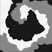
FIG. 14.: A three-armed spiral formed in the inhomogeneously forced FitzHugh-Nagumo system with quenched disorder. The parameters are identical to those in Fig. 13, except for the forcing field parameters which are $\eta_{1}=0$ and $\eta_{2}=2\eta_{0}=0.92$ and $p=q=0.50$. For this forcing field $\bar{\eta}=\eta_{0}=0.46$. The gray-scale indicates the value of $\tan^{-1}(v/u)$. The system size is $512\times 512$; boundary conditions are no-flux.

Depending on $\sigma$, their velocities rank as $v_{12}>v_{23}>v_{31}$ or as $v_{23}>v_{12}>v_{31}$. We note that for all $\sigma$, $v_{12}>v_{31}$. Thus, if a system has initial conditions consisting of two plane fronts, [31 . . . 12] (where . . . represents a region of phase 1), the [12] front will move faster than the [31] front and the distance between the two will decrease. Eventually, the [12] front will closely approach the [31] front and a new stable propagating front consisting of a thin layer of phase 1 connecting phases 3 and 2 will result. We term such a front a compound front and denote it [312]. Similarly, for $\sigma$ values where $v_{23}>v_{12}>v_{31}$, the compound front [123] exists and can be obtained from the starting configuration [12 . . . 23].

FIG. 15.: Front velocity versus $\sigma$ in the forced FHN with periodically updated spatial disorder. Lines of the thinnest width indicate simple fronts: [23] (long dashes), [31](short dashes), [12] (solid line); medium width lines indicate compound fronts: [123] (solid line, exists for $0.99\dots\leq\sigma\leq 1$), [312] (dashes); thick lines indicate pulses: [3123] (dashes, exists for $0.985\dots\leq\sigma\leq 1$), [2312] (dotted line, exists for $5/6\leq\sigma\leq 0.985\dots$). In addition, for $5/6\leq\sigma\leq 0.848\dots$, where $v_{31}>v_{23}$ there should exist a [231] compound front; this front has not been characterized. Velocities were measured in a moving frame in a $200\times 200$ system; the average front position was measured stroboscopically with period $nT_{\mathrm{f}}$ and linear regression was performed to find the slope.

As one might expect, compound fronts cannot be made from a slower moving front following a faster moving front. For example, [231] is not stable; it splits into [23 . . . 31] because $v_{23}>v_{31}$.

The velocities of these compound fronts were measured as a funtion of $\sigma$ and, within our numerical accuracy, were found to lie between the velocities of the two simple fronts from which they were derived (i.e. $v_{12}>v_{312}>v_{31}$ and $v_{23}>v_{123}>v_{12}$ ) (Fig. 15). Depending on $\sigma$ either $v_{312}>v_{23}$ or $v_{23}>v_{312}$. For $v_{312}>v_{23}$ one expects the travelling pulse solution [2312] to be stable, and this is indeed the case, while for $v_{23}>v_{312}$ the pulse [2312] is unstable (it splits into [23] and [312]) while the pulse [3123] is stable. The pulse velocities were measured, they are essentially the same as the velocity of the faster moving component of the pulse.

The existence of stable pulse solutions joing two domains of the same phase raises the question of whether a “one-armed” spiral whose arms consist of the pulse can exist. Figure 16 shows a stable spiral for $\sigma=11/12$, a regime where the velocity ordering is $v_{12}>v_{312}>v_{23}>v_{31}$. It is not a “one-armed” spiral with a [2312] pulse front but could be viewed as a two-armed spiral with arms consisting of phases 3 and 2, with fronts of type [23] and [312]. Since the [312] front velocity is greater than that of the [23] front, one expects that as the waves travel outward phase 3 will shrink and phase 2 will grow, and far from the core the waves will become a train of [2312] pulses.

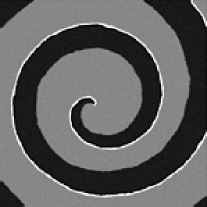
FIG. 16.: A spiral wave in the forced FHN with time-varying spatial disorder with $\sigma=11/12$. The gray-scale indicates the value of $\tan^{-1}(v/u)$. The phases are 1 (light grey ), 2 (dark grey), and 3 (medium grey). The system size is $1024\times 1024$. The noise grain size is $s\times s=L/256\times L/256$. Boundary conditions are no-flux.

Figure 17 shows a spiral for $\sigma=1$. In this regime the velocity ordering is $v_{23}>v_{123}>v_{3123}>v_{12}>v_{312}>v_{31}$. The stable pulse is [3123] rather than [2312]. Far from the core we expect the waves to become a train of [3123] pulses and in Fig. 17 this can indeed be seen to happen.

FIG. 17.: A spiral wave in the forced FHN with time-varying spatial disorder with $\sigma=1$. The gray-scale indicates the value of $\tan^{-1}(v/u)$. The system size is $1024\times 1024$. The noise grain size is $s\times s=L/256\times L/256$. Boundary conditions are no-flux.

The motion of the spiral core was recorded for a realization of the dynamics with $\sigma=11/12$. The trajectory of the core, ${\bf r}_{{\mathrm{c}}}(t)=(x_{{\mathrm{c}}}(t),y_{{\mathrm{c}}}(t))$, describes a “noisy flower pattern” (Fig. 18). Both the periodic looping motion and distortions of the simple flower pattern due to the noise are evident. A plot of $\langle|{\mathbf{r}}_{{\mathrm{c}}}|^{2}\rangle$ vs. $t$ shows periodic behavior with period $\sim 17\;000$, which is also the mean period of rotation of the spiral. In the mean field system with $\eta({\mathbf{r}},t)\equiv\bar{\eta}$ the core is stationary. It is also stationary for the uniformly forced systems with $\eta({\mathbf{r}},t)\equiv\eta_{1}$ and $\eta({\mathbf{r}},t)\equiv\eta_{2}$, the two extreme values of $\eta$ in the dichotomous noise process. Consequently, the core motion is a result of the time-varying spatial disorder of the forcing amplitude field.

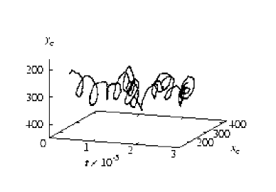
FIG. 18.: Space-time plot of spiral core position versus time for a realization of the forced FHN dynamics with time-varying spatial disorder in a $512\times 512$ system. The updating parameter is $\sigma=11/12$.

We have also investigated time-varying noise where updates occurred at Poisson-distributed intervals instead of periodically. The Poisson distribution used was ${\mathrm{P}r}(t\leq\Delta t_{\ell}\leq t+dt)=(1/\bar{t})e^{-t/\bar{t}}\,dt$ where $\bar{t}=\langle\Delta t_{\ell}\rangle=nT_{{\mathrm{f}}}$. With this choice of $\bar{t}$ the mean time between updates is the same as in the on-resonance periodic updating case discussed previously and corresponds to one period of the entrained system. Thus, if $\Delta t_{\ell}$ are chosen from this distribution then updates of the forcing field occur at times

$$\tau_{k}=\sum_{\ell=1}^{k}\Delta t_{\ell}$$ (39)

in addition to the initial specification of the forcing field at $\tau_{0}$. With these definitions of $\tau_{k}$ in place of Eq. (32), $\eta({\mathbf{r}},t)$ is as given in Eqs. (33)-(34).

We expect that in this system the three phases will be equivalent on average on time scales longer than the average interval between $\eta({\mathbf{r}})$ field updates. The observed spiral shown in Fig. 19 confirms this equivalence. The three arms seen in the figure are approximately equivalent and, when the animation of the dynamics is viewed, this equivalence is preserved in time.

FIG. 19.: A spiral wave in the forced FHN system with time-varying spatial disorder in which the interval between updates is chosen from a Poisson distribution. The gray-scale indicates the value of $\tan^{-1}(v/u)$. The system size is $1024\times 1024$. The noise grain size is $s\times s=L/256\times L/256$. Boundary conditions are no-flux.

V Discussion

We have explored the phenomenology of resonantly forced oscillatory reaction-diffusion systems subject to both quenched and time-varying disorder in the forcing amplitude field. Noteworthy phenomena found when there is quenched disorder are front roughening and spontaneous nucleation of target patterns. Spontaneous nucleation of target patterns arises because diffusion effectively causes averaging of $\gamma({\mathbf{r}})$ ocally over some length scale; hence, the medium locally behaves like a uniform system with the same $\bar{\gamma}$. Alternatively but equivalently, we may describe the dynamics as arising from competition between two regimes selected by the dichotomous forcing values which lie on either side of a bifurcation point. In some spatial regions one regime dominates the dynamics while in other regions the second regime dominates.

For time-varying disorder, the symmetry of the system’s three states is broken, and thus the velocities of different domain walls differ. As a result, travelling front structures other than simple kink-like fronts may exist. These are the compound fronts and pulses. The velocities of the domain walls depend on the phase of the forcing field updating, therefore the updating parameter $\sigma$ selects between regimes in which different sets of compound fronts and pulses exist. This asymmetry among states also leads to spiral waves with inequivalent arms.

Meandering core motion with a noisy flower-like trajectory is seen with time-varying disorder. This core motion arises purely from inhomogeneities in $\eta({\mathbf{r}},t)$ since none of the uniformly forced systems with $\eta({\mathbf{r}},t)\equiv\bar{\eta},\eta_{1},\eta_{2}$ exhibit core meandering.

Some of the effects described herein may arise from the spatial inhomogeneity of the forcing, and not necessarily from its disordered nature. One may also consider regular patterns of inhomogeneous forcing and investigations of this type are in progress. Many of the effects found in this study, such as target pattern nucleation, KPZ front roughening, and front dynamics for time-varying disorder arise from the stochastic nature of the forcing field and would not be found in a system with a regular pattern of forcing.

There are opportunities for further exploration of spatially disordered resonantly forced systems; for example, the effects of noise on various phenomena or bifurcations known in spatially uniform resonantly forced systems have not been studied. Additionally, one may investigate oscillatory systems possessing richer limit cycle dynamics than the relatively uncomplicated examples considered in this paper.

Systems of the types described here could be readily realized in an experimental setup. Standard methodology for investigation of spatial disorder in the light-sensitive excitable BZ reaction involves use of a computer-controlled video projector to project a precisely controllable spatiotemporal pattern of illumination intensity onto the reaction medium. Thus, the only necessary changes are the use of the light-sensitive BZ in the oscillatory regime and reprogramming of the projector to provide a periodic illumination signal incorporating appropriate stochastic spatiotemporal modulation of the light intensity.

REFERENCES

- [1] J. García-Ojalvo and J. M. Sancho, Noise in Spatially Extended Systems (Springer-Verlag, New York, 1999).
- [2] V. Gáspár, G. Bazsa, and M.T. Beck, Z. phys. Chemie (Leipzig) 264 S.43 (1983).
- [3] S. Kádár, J. Wang, and K. Showalter, Nature 391, 770 (1998).
- [4] I. Sendiña-Nadal, A.P. Muñuzuri, D. Vives, V. Pérez-Muñuzuri, J. Casademunt, L. Ramírez-Piscina, J.M. Sancho, and F. Sagués, Phys. Rev. Lett. 80, 5437 (1998).
- [5] I. Sendiña-Nadal, D. Roncaglia, D. Vives, V. Pérez-Muñuzuri, M. Gómez-Gesteira, V. Pérez-Villar, J. Echave, J. Casademunt, L. Ramírez-Piscina, and F. Sagués, Phys. Rev. E 58, R1183 (1998).
- [6] I. Sendiña-Nadal, S. Alonso, V. Pérez-Muñuzuri, M. Gómez-Gesteira, V. Pérez-Villar, L. Ramírez-Piscina, J. Casademunt, J.M. Sancho, and F. Sagués, Phys. Rev. Lett. 84, 2734 (2000).
- [7] Focus issue: Fibrillation in normal ventricular myocardium, Chaos 8(1), 1998.
- [8] P. Jung, A. Cornell-Bell, F. Moss, S. Kadar, J. Wang, and K. Showalter, Chaos 8, 567 (1998).
- [9] J. Maselko and K. Showalter, Physica D 49, 21 (1991).
- [10] P. Jung and G. Mayer-Kress, Chaos 5, 458 (1995).
- [11] P. Jung and G. Mayer-Kress, Phys. Rev. Lett. 74, 2130 (1995).
- [12] M.-N. Chee, S.G. Whittington, and R. Kapral, Physica D 32, 437 (1988).
- [13] V. Petrov, Q. Ouyang, and H.L. Swinney, Nature 388, 655 (1997).
- [14] A. L. Lin, V. Petrov, H. L. Swinney, A. Ardelea, and G. F. Carey, in Pattern Formation in Continous and Coupled Systems; The IMA Volumes in Mathematics and Its Applications, Vol. 115 (Springer-Verlag, New York, 1999).
- [15] A. L. Lin, M. Bertram, K. Martinez, and H. L. Swinney, “Resonant phase patterns in a reaction-diffusion system”, Phys. Rev. Lett., to appear.
- [16] V. Petrov, M. Gustaffson, and H.L. Swinney, “Formation of labyrinthine patterns in a periodically forced reaction-diffusion model” in Conf. Proc. 4th Experimental Chaos Conference (1997).
- [17] A. Belmonte, J.-M. Flesselles, and Q. Ouyang, Europhys. Lett. 35, 665 (1996).
- [18] P. Coullet and K. Emilsson, Physica D 61 119 (1992).
- [19] P. Coullet and K. Emilsson, Physica A 188, 190 (1992).
- [20] P. Coullet, J. Lega, B. Houchmanzadeh, and J. Lajzerowicz, Phys. Rev. Lett. 65, 1352 (1990).
- [21] C. Elphick, A. Hagberg, and E. Meron, Phys. Rev. Lett. 80, 5007 (1998).
- [22] C. Elphick, A. Hagberg, and E. Meron, Phys. Rev. E 59, 5285, (1999).
- [23] H. Chaté, A. Pikovsky, and O. Rudzick, Physica D 131, 17, (1999).
- [24] Y. Kuramoto, Chemical Oscillations, Waves and Turbulence (Springer-Verlag, New York, 1984).
- [25] J.M. Gambaudo, J. Diff. Eq. 57, 172 (1985).
- [26] C. Elphick, G. Iooss, and E. Tirapegui, Phys. Lett. A 120, 459 (1987).
- [27] A.-L. Barabási and H. E. Stanley, Fractal Concepts in Surface Growth (Press Syndicate of the University of Cambridge, New York, 1995).
- [28] R. Kapral, R. Livi, G.-L. Oppo, and A. Politi, Phys. Rev. E 49, 2009 (1994).