Geometric Numerical Integration Applied to
The Elastic Pendulum at Higher Order Resonance

Abstract

In this paper we study the performance of a symplectic numerical integrator based on the splitting method. This method is applied to a subtle problem i.e. higher order resonance of the elastic pendulum. In order to numerically study the phase space of the elastic pendulum at higher order resonance, a numerical integrator which preserves qualitative features after long integration times is needed. We show by means of an example that our symplectic method offers a relatively cheap and accurate numerical integrator.

Keywords. Hamiltonian mechanics, higher-order resonance, elastic pendulum, symplectic numerical integration, geometric integration.
AMS classification. 34C15, 37M15, 65P10, 70H08

1 Introduction

Higher order resonances are known to have a long time-scale behaviour. From an asymptotic point of view, a first order approximation (such as first order averaging) would not be able to clarify the interesting dynamics in such a system. Numerically, this means that the integration times needed to capture such behaviour are significantly increased. In this paper we present a reasonably cheap method to achieve a qualitatively good result even after long integration times.

Geometric numerical integration methods for (ordinary) differential equations ([2, 10, 13]) have emerged in the last decade as alternatives to traditional methods (e.g. Runge-Kutta methods). Geometric methods are designed to preserve certain properties of a given ODE exactly (i.e. without truncation error). The use of geometric methods is particularly important for long integration times. Examples of geometric integration methods include symplectic integrators, volume-preserving integrators, symmetry-preserving integrators, integrators that preserve first integrals (e.g. energy), Lie-group integrators, etc. A survey is given in [10].

It is well known that resonances play an important role in determining the dynamics of a given system. In practice, higher order resonances occur more often than lower order ones, but their analysis is more complicated. In [12], Sanders was the first to give an upper bound on the size of the resonance domain (the region where interesting dynamics takes place) in two degrees of freedom Hamiltonian systems. Numerical studies by van den Broek [16], however, provided evidence that the resonance domain is actually much smaller. In [15], Tuwankotta and Verhulst derived improved estimates for the size of the resonance domain, and provided numerical evidence that for the $4:1$ and the $6:1$ resonances of the elastic pendulum, their estimates are sharp. The numerical method they used in their analysis , however, was not powerful enough to be applied to higher order resonances. In this paper we construct a symplectic integration method, and use it to show numerically that the estimates of the size of the resonance domain in [15] are also sharp for the $4:3$ and the $3:1$ resonances.

Another subtle problem regarding to this resonance manifold is the bifurcation of this manifold as the energy increases. To study this problem numerically one would need a numerical method which is reasonably cheap and accurate after a long integration times.

In this paper we will use the elastic pendulum as an example. The elastic pendulum is a well known (classical) mechanical problem which has been studied by many authors. One of the reasons is that the elastic pendulum can serve as a model for many problems in different fields. See the references in [5, 15]. In itself, the elastic pendulum is a very rich dynamical system. For different resonances, it can serve as an example of a chaotic system, an auto-parametric excitation system ([17]), or even a linearizable system. The system also has (discrete) symmetries which turn out to cause degeneracy in the normal form.

We will first give a brief introduction to the splitting method which is the main ingredient for the symplectic integrator in this paper. We will then collect the analytical results on the elastic pendulum that have been found by various authors. Mostly, in this paper we will be concerned with the higher order resonances in the system. All of this will be done in the next two sections of the paper. In the fourth section we will compare our symplectic integrator with the standard 4-th order Runge-Kutta method and also with an order $7-8$ Runge-Kutta method. We end the fourth section by calculating the size of the resonance domain of the elastic pendulum at higher order resonance.

2 Symplectic Integration

Consider a symplectic space $\Omega=\mathbb{R}^{2n},n\in\mathbb{N}$ where each element $\boldsymbol{\xi}$ in $\Omega$ has coordinate $(\boldsymbol{q},\boldsymbol{p})$ and the symplectic form is $\text{d}\boldsymbol{q}\wedge\text{d}\boldsymbol{p}$. For any two functions $F,G\in\mathcal{C}^{\infty}(\Omega)$ define

$$\{F,G\}=\sum\limits_{1}^{n}\left(\frac{\partial F}{\partial q_{j}}\frac{\partial G}{\partial p_{j}}-\frac{\partial G}{\partial q_{j}}\frac{\partial F}{\partial p_{j}}\right)\in\mathcal{C}^{\infty}(\Omega),$$

which is called the Poisson bracket of $F$ and $G$. Every function $H\in\mathcal{C}^{\infty}(\Omega)$ generates a (Hamiltonian) vector field defined by $\{q_{i},H\},\{p_{i},H\},i=1,\ldots,n$. The dynamics of $H$ is then governed by the equations of motion of the form

$$\begin{split}\dot{q_{i}}=&\{q_{i},H\}\\ \dot{p_{i}}=&\{p_{i},H\},\quad i=1,\ldots,n.\end{split}$$

Let $X$ and $Y$ be two Hamiltonian vector fields, defined in $\Omega$, associated with Hamiltonians $H_{\scriptscriptstyle X}$ and $H_{\scriptscriptstyle Y}$ in $\mathcal{C}^{\infty}(\Omega)$ respectively. Consider another vector field $[X,Y]$ which is just the commutator of the vector fields $X$ and $Y$ . Then $[X,Y]$ is also a Hamiltonian vector field with Hamiltonian $H_{\scriptscriptstyle[X,Y]}=\{H_{\scriptscriptstyle X},H_{\scriptscriptstyle Y}\}$. See for example [1, 7, 11] for details.

We can write the flow of the Hamiltonian vector fields $X$ as

$$\varphi_{{\scriptscriptstyle X};t}=\text{ exp}(tX)\equiv I+tX+\frac{1}{2!}(tX)^{2}+\frac{1}{3!}(tX)^{3}+\cdots$$

(and so does the flow of $Y$). By the BCH formula, there exists a (formal) Hamiltonian vector field $Z$ such that

$$Z=(X+Y)+\frac{t}{2}[X,Y]+\frac{t^{2}}{12}\left([X,X,Y]+[Y,Y,X]\right)+O(t^{3})$$ (1)

and $\text{exp}(tZ)=\text{exp}(tX)\text{exp}(tY)$, where $[X,X,Y]=[X,[X,Y]]$ , and so on. Moreover, Yoshida (in [19]) shows that $\text{exp}(tX)\text{exp}(tY)\text{exp}(tX)=\text{exp}(tZ),$ where

$$Z=(2X+Y)+\frac{t^{2}}{6}\left([Y,Y,X]-[X,X,Y]\right)+O(t^{4}).$$ (2)

We note that in terms of the flow, the multiplication of the exponentials above means composition of the corresponding flow, i.e. $\varphi_{{\scriptscriptstyle Y};t}\circ\varphi_{{\scriptscriptstyle X};t}$.

Let $\tau\in\mathbb{R}$ be a small positive number and consider a Hamiltonian system with Hamiltonian $H(\boldsymbol{\xi})=H_{\scriptscriptstyle X}(\boldsymbol{\xi})+H_{\scriptscriptstyle Y}(\boldsymbol{\xi})$, where $\boldsymbol{\xi}\in\Omega$, and $\dot{\boldsymbol{\xi}}=X+Y$. Using (1) we have that $\varphi_{{\scriptscriptstyle Y};\tau}\circ\varphi_{{\scriptscriptstyle X};\tau}$ is (approximately) the flow of a Hamiltonian system

$$\dot{\boldsymbol{\xi}}=(X+Y)+\frac{\tau}{2}[X,Y]+\frac{\tau^{2}}{12}\left([X,X,Y]+[Y,Y,X]\right)+O(\tau^{3}),$$

with Hamiltonian

$$H_{\tau}=H_{\scriptscriptstyle X}+H_{\scriptscriptstyle Y}+\frac{\tau}{2}\left\{H_{\scriptscriptstyle X},H_{\scriptscriptstyle Y}\right\}+\frac{\tau^{2}}{12}\left(\left\{H_{\scriptscriptstyle X},H_{\scriptscriptstyle X},H_{\scriptscriptstyle Y}\right\}+\left\{H_{\scriptscriptstyle Y},H_{\scriptscriptstyle Y},H_{\scriptscriptstyle X}\right\}\right)+O(\tau^{3}).$$

Note that $\{H,K,F\}=\{H,\{K,F\}\}$. This mean that $H-H_{\tau}=O(\tau)$ or, in other words

$$\varphi_{{\scriptscriptstyle Y};\tau}\circ\varphi_{{\scriptscriptstyle X};\tau}=\varphi_{\scriptscriptstyle X+Y}(\tau)+O(\tau^{2}).$$ (3)

As before and using (2), we conclude that

$$\varphi_{{\scriptscriptstyle X};\frac{\tau}{2}}\circ\varphi_{{\scriptscriptstyle Y};\tau}\circ\varphi_{{\scriptscriptstyle X};\frac{\tau}{2}}=\varphi_{\scriptscriptstyle X+Y}(\tau)+O(\tau^{3}).$$ (4)

Suppose that $\psi_{{\scriptscriptstyle X};\tau}$ and $\psi_{{\scriptscriptstyle Y};\tau}$ are numerical integrators of system $\dot{\boldsymbol{\xi}}=X$ and $\dot{\boldsymbol{\xi}}=Y$ (respectively). We can use symmetric composition (see [8]) to improve the accuracy of $\psi_{{\scriptscriptstyle X+Y};\tau}$. If $\psi_{{\scriptscriptstyle Y};\tau}$ and $\psi_{{\scriptscriptstyle X};\tau}$ are symplectic, then the composition forms a symplectic numerical integrator for $X+Y$. See [13] for more discussion; also [10] for references. If we can split $H$ into two (or more) parts which Poisson commute with each other (i.e. the Poisson brackets between each pair vanish), then we have $H=H_{\tau}$. This implies that in this case the accuracy of the approximation depends only on the accuracy of the integrators for $X$ and $Y$. An example of this case is when we are integrating the Birkhoff normal form of a Hamiltonian system.

3 The Elastic Pendulum

Consider a spring with spring constant $s$ and length $l_{\circ}$ to which a mass $m$ is attached. Let $g$ be the gravitational constant and $l$ the length of the spring under load in the vertical position, and let $r$ be the distance between the mass $m$ and the suspension point. The spring can both oscillate in the radial direction and swing like a pendulum. This is called the elastic pendulum. See Figure (1) for illustration and [15] (or [18]) for references.

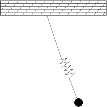
Figure 1: The elastic pendulum.

The phase space is $\mathbb{R}^{4}$ with canonical coordinate $\boldsymbol{\xi}=(z,\varphi,p_{z},p_{\varphi})$, where $z=(r-l_{\circ})/l_{\circ}$. Writing the linear frequencies of the Hamiltonian as $\omega_{z}=\sqrt{s/m}$ and $\omega_{\varphi}=\sqrt{g/l}$, the Hamiltonian of the elastic pendulum becomes

$$H=\frac{1}{2\sigma}\left(p_{z}^{2}+\frac{p_{\varphi}^{2}}{(z+1)^{2}}\right)+\frac{\sigma}{2}{\omega_{z}}^{2}\left(z+\left(\frac{\omega_{\varphi}}{\omega_{z}}\right)^{2}\right)^{2}-\sigma{\omega_{\varphi}}^{2}(z+1)\cos\varphi,$$ (5)

where $\sigma=ml^{2}$. By choosing the right physical dimensions, we can scale out $\sigma$. We remark that for the elastic pendulum as illustrated in Figure 1, we have $\omega_{z}\leq\omega_{\varphi}$. See [15] for details. It is clear that this system possesses symmetry

$$T:(z,\varphi,p_{z},p_{\varphi},t)\mapsto(z,-\varphi,p_{z},-p_{\varphi},t)$$ (6)

and the reversing symmetries

$$\begin{array}[]{c}R_{1}:(z,\varphi,p_{z},p_{\varphi},t)\mapsto(z,\varphi,-p_{z},-p_{\varphi},-t),\\ R_{2}:(z,\varphi,p_{z},p_{\varphi},t)\mapsto(z,-\varphi,-p_{z},p_{\varphi},-t).\end{array}$$ (7)

If there exist two integers $k_{1}$ and $k_{2}$ such that $k_{1}\omega_{z}+k_{2}\omega_{\varphi}=0$, then we say $\omega_{z}$ and $\omega_{\varphi}$ are in resonance. Assuming $(|k_{1}|,|k_{2}|)=1$, we can divide the resonances in two types, e.g. lower order resonance if $|k_{1}|+|k_{2}|<5$ and higher order resonance if $|k_{1}|+|k_{2}|\geq 5$. In the theory of normal forms, the type of normal form of the Hamiltonian is highly dependent on the type of resonance in the system. See [1].

In general, the elastic pendulum has at least one fixed point which is the origin of phase space. This fixed point is elliptic. For some of the resonances, there is also another fixed point which is of the saddle type, i.e. $(z,\varphi,p_{z},p_{\varphi})=(-2(\omega_{\varphi}/\omega_{z})^{2},\pi,0,0)$. From the definition of $z$, it is clear that the latter fixed point only exists for $\omega_{z}/\omega_{\varphi}>\sqrt{2}$. The elastic pendulum also has a special periodic solution in which $\varphi=p_{\varphi}=0$ (the normal mode). This normal mode is an exact solution of the system derived from (5). We note that there is no nontrivial solution of the form $(0,\varphi(t),0,p_{\varphi}(t))$.

Now we turn our attention to the neighborhood of the origin. We refer to [15] for the complete derivation of the following Taylor expansion of the Hamiltonian (we have dropped the bar)

$$H=H_{2}+\varepsilon H_{3}+\varepsilon^{2}H_{4}+\varepsilon^{3}H_{5}+\cdots,$$ (8)

with

$$\begin{split}H_{2}=&\textstyle\frac{1}{2}\omega_{z}\left(z^{2}+p_{z}^{2}\right)+\frac{1}{2}\omega_{\varphi}\left(\varphi^{2}+p_{\varphi}^{2}\right)\\ H_{3}=&\textstyle\frac{\omega_{\varphi}}{\sqrt{\omega_{z}}}\left(\frac{1}{2}z\varphi^{2}-zp_{\varphi}^{2}\right)\\ H_{4}=&\textstyle\left(\frac{3}{2}\frac{\omega_{\varphi}}{\omega_{z}}z^{2}p_{\varphi}^{2}-\frac{1}{24}\varphi^{4}\right)\\ H_{5}=&\textstyle-\frac{1}{\sqrt{\omega_{z}}}\left(\frac{1}{24}z\varphi^{4}+2\frac{\omega_{\varphi}}{\omega_{z}}z^{3}p_{\varphi}^{2}\right)\\ &\qquad\vdots\end{split}$$

In [17] the $2:1$-resonance of the elastic pendulum has been studied intensively. At this specific resonance, the system exhibits an interesting phenomenon called auto-parametric excitation, e.g. if we start at any initial condition arbitrarily close to the normal mode, then we will see energy interchanging between the oscillating and swinging motion. In [3], the author shows that the normal mode solution (which is the vertical oscillation) is unstable and therefore, gives an explanation of the auto-parametric behavior.

Next we consider two limiting cases of the resonances, i.e. when $\omega_{z}/\omega_{\varphi}\rightarrow\infty$ and $\omega_{z}/\omega_{\varphi}\rightarrow 1$. The first limiting case can be interpreted as a case with a very large spring constant so that the vertical oscillation can be neglected. The spring pendulum then becomes an ordinary pendulum; thus the system is integrable. The other limiting case is interpreted as the case where $l_{\circ}=0$ (or very weak spring) . Using the transformation $r=l(z+1)$, $x=r\cos\varphi$ and $y=r\sin\varphi,$ we transform the Hamiltonian (5) to the Hamiltonian of the harmonic oscillator. Thus this case is also integrable. Furthermore, in this case all solutions are periodic with the same period which is known as isochronism. This means that we can remove the dependence of the period of oscillation of the mathematical pendulum on the amplitude, using this specific spring. We note that this isochronism is not derived from the normal form (as in [18]) but exact.

All other resonances are higher order resonances. In two degrees of freedom (which is the case we consider), for fixed small energy the phase space of the system near the origin looks like the phase space of decoupled harmonic oscillator. A consequence of this fact is that in the neighborhood of the origin, there is no interaction between the two degrees of freedom. The normal mode (if it exists), then becomes elliptic (thus stable).

Another possible feature of this type of resonance is the existence of a resonance manifold containing periodic solutions (see [4] paragraph 4.8). We remark that the existence of this resonance manifold does not depend on whether the system is integrable or not. In the resonance domain (i.e. the neighborhood of the resonant manifold), interesting dynamics (in the sense of energy interchanging between the two degrees of freedom) takes place (see [12]). Both the size of the domain where the dynamics takes place and the time-scale of interaction are characterized by $\varepsilon$ and the order of the resonance, i.e. the estimate of the size of the domain is

$$d_{\varepsilon}=O\left(\varepsilon^{\frac{m+n-4}{2}}\right)$$ (9)

and the time-scale of interactions is $O(\varepsilon^{-\frac{m+n}{2}})$ for $\omega_{z}:\omega_{\varphi}=m:n$ with $(m,n)=1$. We note that for some of the higher order resonances where $\omega_{z}/\omega_{\varphi}\approx 1$ the resonance manifold fails to exist. See [15] for details.

4 Numerical Studies on the Elastic Pendulum

One of the aims of this study is to construct a numerical Poincaré map ($\mathcal{P}$) for the elastic pendulum in higher order resonance. As is explained in the previous section, interesting dynamics of the higher order resonances takes place in a rather small part of phase space. Moreover, the interaction time-scale is also rather long. For these two reasons, we need a numerical method which preserves qualitative behavior after a long time of integration. Obviously by decreasing the time step of any standard integrator (e.g. Runge-Kutta method), we would get a better result. As a consequence however, the actual computation time would become prohibitively long. Under these constraints, we would like to propose by means of an example that symplectic integrators offer reliable and reasonably cheap methods to obtain qualitatively good phase portraits.

We have selected four of the most prominent higher order resonances in the elastic pendulum. For each of the chosen resonances, we derive its corresponding equations of motion from (8). This is done because the dependence on the small parameter $\varepsilon$ is more visible there than in (5). Also from the asymptotic analysis point of view, we know that (8) truncated to a sufficient degree has enough ingredients of the dynamics of (5).

The map $\mathcal{P}$ is constructed as follows. We choose the initial values $\boldsymbol{\xi_{\circ}}$ in such a way that they all lie in the approximate energy manifold $H_{2}=E_{\circ}\in\mathbb{R}$ and in the section $\Sigma=\{\boldsymbol{\xi}=(z,\varphi,p_{z},p_{\varphi})|z=0,p_{z}>0\}$. We follow the numerically constructed trajectory corresponding to $\boldsymbol{\xi_{\circ}}$ and take the intersection of the trajectory with section $\Sigma$. The intersection point is defined as $\mathcal{P}(\boldsymbol{\xi_{\circ}})$. Starting from $\mathcal{P}(\boldsymbol{\xi_{\circ}})$ as an initial value, we go on integrating and in the same way we find $\mathcal{P}^{2}(\boldsymbol{\xi_{\circ}})$, and so on.

The best way of measuring the performance of a numerical integrator is by comparing with an exact solution. Due to the presence of the normal mode solution (as an exact solution), we can check the performance of the numerical integrator in this way (we will do this in section 4.2) . Nevertheless, we should remark that none of the nonlinear terms play a part in this normal mode solution. Recall that the normal mode is found in the invariant manifold $\{(z,\varphi,p_{z},p_{\varphi}|\varphi=p_{\varphi}=0\}$ and in this manifold the equations of motion of (8) are linear.

Another way of measuring the performance of an integrator is to compare it with other methods. One of the best known methods for time integration are the Runge-Kutta methods (see [6]). We will compare our integrator with a higher order ($7$-$8$ order) Runge-Kutta method (RK78). The RK78 is based on the method of Runge-Kutta-Felbergh ([14]). The advantage of this method is that it provides step-size control. As is indicated by the name of the method, to choose the optimal step size it compares the discretizations using $7$-th order and $8$-th order Runge-Kutta methods. A nice discussion on lower order methods of this type, can be found in [14] pp. 448-454. The coefficients in this method are not uniquely determined. For RK78 that we used in this paper, the coefficients were calculated by C. Simo from the University of Barcelona. We will also compare the symplectic integrator (SI) to the standard $4$-th order Runge-Kutta method.

We will first describe the splitting of the Hamiltonian which is at the core of the symplectic integration method in this paper. By combining the flow of each part of the Hamiltonian, we construct a $4$-th order symplectic integrator. The symplecticity is obvious since it is the composition of exact Hamiltonian flows. Next we will show the numerical comparison between the three integrators, RK78, SI and RK4. We compare them to an exact solution. We will also show the performance of the numerical integrators with respect to energy preservation. We note that SI are not designed to preserve energy (see [10]). Because RK78 is a higher order method (thus more accurate), we will also compare the orbit of RK4 and SI. We will end this section with results on the size of the resonance domain calculated by the SI method.

4.1 The Splitting of the Hamiltonian

Consider again the expanded Hamiltonian of the elastic pendulum (8). We split this Hamiltonian into integrable parts: $H=H^{1}+H^{2}+H^{3}$, where

$$\begin{split}H^{1}=&\varepsilon\frac{\omega_{\varphi}}{2\sqrt{\omega_{z}}}z\varphi^{2}-\varepsilon^{2}\frac{1}{24}\varphi^{4}-\varepsilon^{3}\frac{1}{24\sqrt{\omega_{z}}}z\varphi^{4}+\cdots\\ H^{2}=&-\varepsilon\frac{\omega_{\varphi}}{\sqrt{\omega_{z}}}zp_{\varphi}^{2}+\varepsilon^{2}\frac{3}{2}\frac{\omega_{\varphi}}{\omega_{z}}z^{2}p_{\varphi}^{2}-\varepsilon^{3}\frac{2\omega_{\varphi}}{\omega_{z}\sqrt{\omega_{z}}}z^{3}p_{\varphi}^{2}+\cdots\\ H^{3}=&\textstyle\frac{1}{2}\omega_{z}\left(z^{2}+p_{z}^{2}\right)+\frac{1}{2}\omega_{\varphi}\left(\varphi^{2}+p_{\varphi}^{2}\right).\end{split}$$ (10)

Note that the equations of motion derived from each part of the Hamiltonian can be integrated exactly; thus we know the exact flow $\varphi_{1;\tau}$, $\varphi_{2:\tau}$, and $\varphi_{3;\tau}$ corresponding to $H^{1}$,$H^{2}$, and $H^{3}$ respectively. This splitting has the following advantages.

• It preserves the Hamiltonian structure of the system.

• It preserves the symmetry (6) and reversing symmetries (7) of $H$.

• $H^{1}$ and $H^{2}$ are of $O(\varepsilon)$ compared with $H$ (or $H^{3}$).

Note that, for each resonance we will truncate (10) up to and including the degree where the resonant terms of the lowest order occur.

We define

$$\varphi_{\tau}=\varphi_{1;\tau/2}\circ\varphi_{2;\tau/2}\circ\varphi_{3;\tau}\circ\varphi_{2;\tau/2}\circ\varphi_{1;\tau/2}.$$ (11)

From section 2 we know that this is a second order method. Next we define $\gamma=1/(2-\sqrt[3]{2})$ and $\psi_{\tau}=\varphi_{\gamma\tau}\circ\varphi_{(1-2\gamma)\tau}\circ\varphi_{\gamma\tau}$ to get a fourth order method. This is known as the generalized Yoshida method (see [10]). By, Symplectic Integrator (SI) we will mean this fourth order method. This composition preserves the symplectic structure of the system, as well as the symmetry (6) and the reversing symmetries (7). This is in contrast with the Runge-Kutta methods which only preserves the symmetry (6), but not the symplectic structure, nor the reversing symmetries (7). As a consequence the Runge-Kutta methods do not preserve the KAM tori caused by symplecticity or reversibility.

4.2 Numerical Comparison between RK4, RK78 and SI

We start by comparing the three numerical methods, i.e. RK4, RK78, and SI. We choose the $4:1$-resonance, which is the most prominent higher order resonance, as a test problem. We fix the value of the energy ($H_{2}$) to be $5$ and take $\varepsilon=0.05$. Starting at the initial condition $z(0)=0,\varphi(0)=0,p_{z}=\sqrt{5/2},$ and $p_{\varphi}(0)=0$, we know that the exact solution we are approximating is given by $(\sqrt{5/2}\;\sin(4t),0,\sqrt{5/2}\;\cos(4t),0)$. We integrate the equations of motion up to $t=10^{5}$ seconds and keep the result of the last $10$ seconds to have time series $\overline{z}(t_{n})$ and $\overline{p_{z}}(t_{n})$ produced by each integrator. Then we define a sequence $s_{n}=99990+5n/100,n=0,1,\ldots,200$. Using an interpolation method, for each of the time series we calculate the numerical $\overline{z}(s_{n})$. In figure 2 we plot the error function $\overline{z}(s_{n})-z(s_{n})$ for each integrator.

Figure 2: Plots of the error function $\overline{z}(s_{n})-z(s_{n})$ against time. The upper figure is the result of RK4, the middle figure is RK78 and the lower figure is of SI. The time of integration is $10^{5}$ with a time step for RK4 and SI of $0.025$.

The plots in Figure in 2 clearly indicate the superiority of RK78 compared with the other methods (due to the higher order method). The error generated by RK78 is of order $10^{-7}$ for an integration time of $10^{5}$ seconds. The minimum time step taken by RK78 is $0.0228$ and the maximum is $0.0238$. The error generated by SI on the other hand, is of order $10^{-5}$. The CPU time of RK78 during this integration is $667.75$ seconds. SI completes the computation after $446.72$ seconds while RK4 only needs $149.83$ seconds.

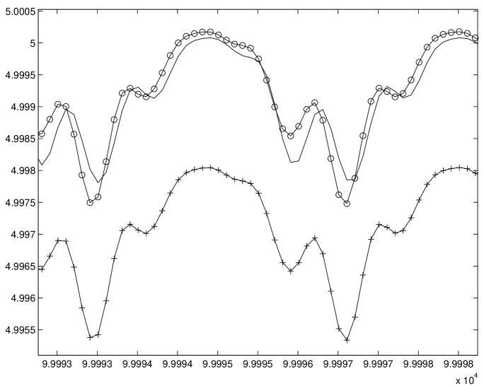
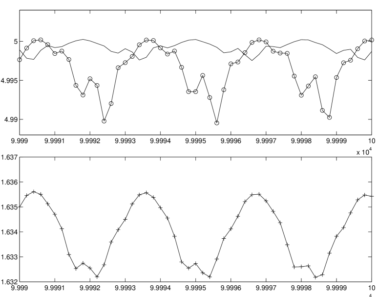
Figure 3: Plots of the energy against time. The solid line represents the results from SI. The line with ’+’ represents the results from RK4 and the line with ’$\circ$’ represents the results from RK78. On the left hand plot, we show the results of all three methods with the time step $0.01$. The time step in the right hand plots is $0.05$. The results from RK4 are plotted seperately since the energy has decreased significantly compared to the other two methods.

We will now measure how well these integrators preserve energy. We start integrating from an initial condition $z(0)=0$, $\varphi(0)=1.55$, $p_{\varphi}(0)=0$ and $p_{z}(0)$ is determined from $H^{3}=5$ (in other word we integrate on the energy manifold $H=5+O(\varepsilon)$). The small parameter is $\varepsilon=0.05$ and we integrate for $t=10^{5}$ seconds.

For RK78, the integration takes $667.42$ second of CPU time. For RK4 and SI we used the same time step, that is $10^{-2}$. RK4 takes $377.35$ seconds while SI takes $807.01$ seconds of CPU time. It is clear that SI, for this size of time step, is inefficient with regard to CPU time. This is due to the fact that to construct a higher order method we have to compose the flow several times. We plot the results of the last $10$ seconds of the integrations in Figure 3. We note that in these $10$ seconds, the largest time step used by RK78 is 0.02421…while the smallest is 0.02310…. It is clear from this, that even though the CPU time of RK4 is very good, the result in the sense of conservation of energy is rather poor relative to the other methods.

We increase the time step to $0.05$ and integrate the equations of motion starting at the same initial condition and for the same time. The CPU time of SI is now $149.74$ while for the RK4 it is $76.07$. Again, in Figure 3 (the right hand plots) we plot the energy against time. A significant difference between RK4 and SI then appears in the energy plots. The results of symplectic integration are still good compared with the higher order method RK78. On the other hand, the results from RK4 are far below the other two.

4.3 Computation of the Size of the Resonance Domain

Finally, we calculate the resonance domain for some of the most prominent higher order resonances for the elastic pendulum. In Figure 4 we give an example of the resonance domain for the $4:1$ resonance. We note that RK4 fails to produce the section.

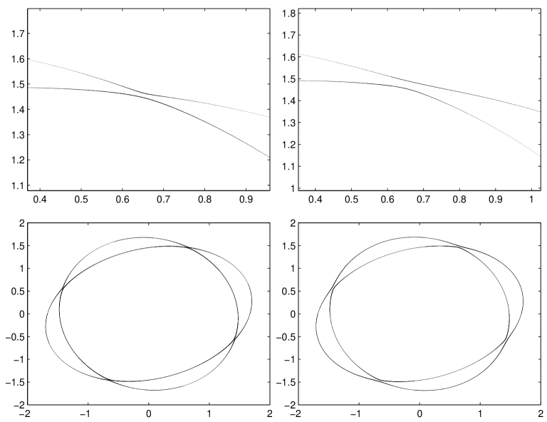
Figure 4: Resonance domain for the $4:1$-resonance. The plots on the left are the results from SI while the right hand plots are the results from RK78. The vertical axis is the $p_{\varphi}$ axis and the horizontal axis is $\varphi$. The time step is $0.05$ and $\varepsilon=0.05$. In the top figures, we blow up a part of the pictures underneath.

On the other hand, the results from SI are still accurate. We compare the results from SI and RK78 in Figure 4. After $5\times 10^{3}$ seconds, one loop in the plot is completed. For that time of integration, RK78 takes $34.92$ seconds of CPU time, while SI takes only $16.35$ seconds. This is very useful since to calculate for smaller values of $\varepsilon$ and higher resonance cases, the integration time is a lot longer which makes it impractical to use RK78.

In Table 1 we list the four most prominent higher order resonances for the elastic pendulum. This table is adopted from [15] where the authors list six of them.

Resonance	Resonant	Analytic	Numerical	Error
	part	$\log_{\varepsilon}(d_{\varepsilon})$	$\log_{\varepsilon}(d_{\varepsilon})$
$4:1$	$H_{5}$	$1/2$	$0.5091568$	0.004
$6:1$	$H_{7}$	$3/2$	$1.5079998$	0.05
$4:3$	$H_{7}$	$3/2$	$1.4478968$	0.09
$3:1$	$H_{8}$	$2$	$2.0898136$	0.35

Table 1: Comparison between the analytic estimate and the numerical computation of the size of the resonance domain of four of the most prominent higher order resonances of the elastic pendulum. The second column of this table indicates the part of the expanded Hamiltonian in which the lowest order resonant terms are found.

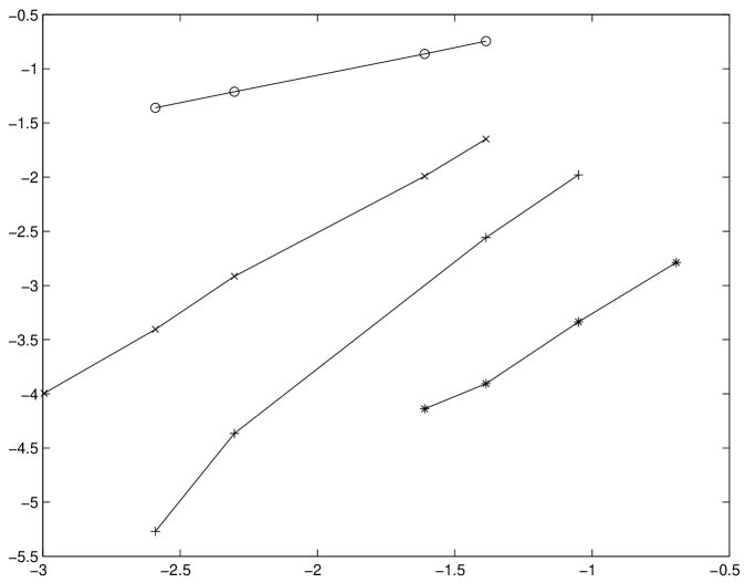
Figure 5: Plots of $\log(d_{\varepsilon})$ against $\log(\varepsilon)$ for various resonances. The $4:1$-resonance is plotted using ’$-\circ$’, the $3:1$-resonance is using ’$-+$’, the $4:3$-resonance is using ’$-\times$’ and the $6:1$ resonance is using ’$-\ast$’.

The numerical size of the domain in table 1 is computed as follows. We first draw several orbits of the Poincaré maps $\mathcal{P}$. Using a twist map argument, we can locate the resonance domain. By adjusting the initial condition manually, we then approximate the heteroclinic cycle of $\mathcal{P}$. See figure 4 for illustration. Using interpolation we construct the function $r_{o}(\theta)$ which represent the distance of a point in the outer cycle to the origin and $\theta$ is the angle with respect to the positive horizontal axis. We do the same for the inner cycle and then calculate $\max_{\theta}|r_{o}(\theta)-r_{i}(\theta)|$. The higher the resonance is, the more difficult to compute the size of the domain in this way.

For resonances with very high order, manually approximating the heteroclinic cycles would become impractical, and one could do the following. First we have to calculate the location of the fixed points of the iterated Poincaré maps numerically. Then we can construct approximations of the stable and unstable manifolds of one of the saddle points. By shooting to the next saddle point, we can make corrections to the approximate stable and unstable manifold of the fixed point.

5 Discussion

In this section we summarize the previous sections. First the performance of the integrators is summarized in table 2.

		Integrators
		RK4	RK78	SI
	CPU time ($\Delta t\approx 0.025,t=10^{5}$ sec.)	$149.83$ sec.	$667.75$ sec.	$446.72$ sec.
The $4:1$	Preservation of $H$ ($t=10^{5}$ sec.)	Poor	Good	Good
resonance	Orbital Quality	Poor	Very good	Good
	Section Quality	—	Good	Good
The $6:1$	Orbital Quality	Poor	Good	Good
resonance	Section Quality	—	Good	Good
The $4:3$	Orbital Quality	Poor	Good	Good
resonance	Section Quality	—	—	Good
The $3:1$	Orbital Quality	Poor	Poor	Good
resonance	Section Quality	—	—	Good

Table 2: Summary of the performance of the integrators. A bar — indicates that it is not feasible to obtain a surface of section for this resonance using this integrator.

As indicated in table 2, for the $4:3$ and the $3:1$ resonances, the higher order Runge-Kutta method fails to produce the section. This is caused by the dissipation term, artificially introduced by this numerical method, which after a long time of integration starts to be more significant. On the other hand, we conclude that the results of our symplectic integrator are reliable. This conclusion is also supported by the numerical calculations of the size of the resonance domain (listed in Table 2).

In order to force the higher order Runge-Kutta method to be able to produce the section, one could also do the following. Keeping in mind that RK78 has automatic step size control based on the smoothness of the vector field, one could manually set the maximum time step for RK78 to be smaller than $0.02310$. This would make the integration times extremely long however.

We should remark that in this paper we have made a number of simplifications. One is that we have not used the original Hamiltonian. The truncated Taylor expansion of (5) is polynomial. Somehow this may have a smoothing effect on the Hamiltonian system. It would be interesting to see the effect of this simplification on the dynamics of the full system. Another simplification is that, instead of choosing our initial conditions in the energy manifold $H=C$, we are choosing them in $H^{3}=C$. By using the full Hamiltonian instead of the truncated Taylor expansion of the Hamiltonian, it would become easy to choose the initial conditions in the original energy manifold. Nevertheless, since in this paper we always start in the section $\Sigma$, we know that we are actually approximating the original energy manifold up to order $\varepsilon^{2}$.

We also have not used the presence of the small parameter $\varepsilon$ in the system. As noted in [9], it may be possible to improve our symplectic integrator using this small parameter. Still related to this small parameter, one also might ask whether it would be possible to go to even smaller values of $\varepsilon$. In this paper we took $e^{-3}<\varepsilon<e^{-0.5}$. As noted in the previous section, the method that we apply in this paper can not be used for computing the size of the resonance domain for very high order resonances. This is due to the fact that the resonance domain then becomes exceedingly small. This is more or less the same difficulty we might encounter if we decrease the value of $\varepsilon$.

Another interesting posibility is to numerically follow the resonance manifold as the energy increases. As noted in the introduction, this is numerically difficult problem. Since this symplectic integration method offers a cheap and accurate way of producing the resonance domain, it might be posible to numerically study the bifurcation of the resonance manifold as the energy increases. Again, we note that to do so we would have to use the full Hamiltonian.

Acknowledgements

J.M. Tuwankotta thanks the School of Mathematical and Statistical Sciences, La Trobe University, Australia for their hospitality when he was visiting the university. Thanks to David McLaren of La Trobe University, and Ferdinand Verhulst, Menno Verbeek and Michiel Hochstenbach of Universiteit Utrecht, the Netherlands for their support and help during the execution of this research. Many thanks also to Santi Goenarso for every support she has given.

We are grateful to the Nederlandse Organisatie voor Wetenschappelijk Onderzoek (NWO) and to the Australian Research Council (ARC) for financial support.

References

- [1] Arnol’d, V.I., Mathematical Methods of Classical Mechanics, Springer-Verlag, New York etc., 1978.
- [2] Budd, C.J., Iserles, A., eds. Geometric Integration, Phil. Trans. Roy. Soc. 357 A, pp. 943-1133, 1999.
- [3] Duistermaat, J.J., On Periodic Solutions near Equilibrium Points of Conservative Systems, Archive for Rational Mechanics and Analysis, vol. 45, num. 2, 1972.
- [4] Guckenheimer, J., Holmes, P., Nonlinear Oscillations, Dynamical Systems, and Bifurcations of Vector Fields, Springer-Verlag, New York etc., 1983.
- [5] Georgiou, I.,T., On the global geometric structure of the dynamics of the elastic pendulum, Nonlinear Dynamics 18,no. 1, pp. 51-68, 1999.
- [6] Hairer, E., Nørsett, S.P., Wanner, G., Solving Ordinary Differential Equations, Springer-Verlag, New York etc.,1993.
- [7] Marsden,J.E., Ratiu, T.S., Introduction to Mechanics and Symmetry,Text in Applied Math. 17, Springer-Verlag, New York etc., 1994.
- [8] McLachlan, R.I., On the Numerical Integration of Ordinary Differential Equations by Symmetric Composition Methods, SIAM J. Sci. Comput., vol. 16, no.1, pp. 151-168, 1995.
- [9] McLachlan, R.I., Composition Methods in the Presence of Small Parameters, BIT, no.35, pp. 258-268, 1995.
- [10] McLachlan, R.I., Quispel, G.R.W., Six Lectures on The Geometric Integration of ODEs, to appear in Foundations of Computational Mathematics, Oxford 1999, eds. R.A. De Vore et. al., Cambridge University Press. , Cambridge.
- [11] Olver, P.J., Applications of Lie Groups to Differential Equations, Springer-Verlag, New York etc. 1986.
- [12] Sanders, J.A.,Are higher order resonances really interesting?, Celestial Mech. 16, pp. 421-440, 1978.
- [13] Sanz-Serna, J.-M., Calvo, M.-P Numerical Hamiltonian Problems, Chapman Hall, 1994.
- [14] Stoer, J., Bulirsch, R.,Introduction to Numerical Analysis, 2nd ed., Text in Applied Math. 12, Springer-Verlag, 1993.
- [15] Tuwankotta, J.M., Verhulst, F., Symmetry and Resonance in Hamiltonian Systems, to appear in SIAM Journal on Applied Math..
- [16] van den Broek, B., Studies in Nonlinear Resonance, Applications of Averaging, Ph.D. Thesis University of Utrecht, 1988.
- [17] van der Burgh, A.H.P., On The Asymptotic Solutions of the Differential Equations of the Elastic Pendulum, Journal de Mécanique, vol. 7. no. 4, pp. 507-520, 1968.
- [18] van der Burgh, A.H.P., On The Higher Order Asymptotic Approximations for the Solutions of the Equations of Motion of an Elastic Pendulum, Journal of Sound and Vibration 42, pp. 463-475, 1975.
- [19] Yoshida, H., Construction of Higher Order Symplectic Integrators, Phys. Lett. 150A, pp. 262-268, 1990.