Temporal Structures in Shell Models.

Abstract

The intermittent dynamics of the turbulent GOY shell-model is characterised by a single type of burst-like structure, which moves through the shells like a front. This temporal structure is described by the dynamics of the instantaneous configuration of the shell-amplitudes revealing a approximative chaotic attractor of the dynamics.

1 Introduction

One of the main goals in current turbulence research is to understand the effect of intermittency in turbulence. It has long been known that intermittency produces corrections to the classical Kolmogorov $-5/3$ scaling law and to other moments of the energy spectrum in the inertial range [1, 2]. Still very little is known about the intense intermittent structures found in turbulent flows [3].
Over the last decade turbulent shell-models have been studied intensively because of their simplicity and excellent agreement of their statistics in comparison with that of experimentally measured turbulence [4, 5, 6, 7, 8, 9]. In a way these models reproduce the statistics far better than expected from their simplicity, so the general idea has been to reveal the nature of the dynamics of these models and then afterwards relate this experiences to the full problem of turbulence.
While the main approach to shell models has been statistical, much can be learned from the study of the temporal structures naturally arising in the model. Because of the intense dynamics during these temporal events they are called bursts. Only recently have these temporal structures been thoroughly studied together with the nature of their creation [10, 11]. Among the large numbers and types of different shell-models the present work is based on the successful GOY shell-model [4, 5].
The paper is organised as follows: The first part gives a detailed description of the bursts of the standard GOY-model. The second part shows that an approximative chaotic attractor of the model exists expressed by the collective dynamics of the neighbouring shells.

2 The GOY-model

All shell-models simulate the flow of energy through wavenumber space in fully developed turbulence. The models consist of a system of coupled ordinary differential equations where the energy is injected into the low wave-numbers by a constant forcing term. The energy then cascades up to the high wave-numbers by means of a coupling term where it is dissipated away by a viscosity term.

2.1 Construction

In the GOY model wave-number space is divided into $N$ separate shells with characteristic wavenumbers $k_{n}=k_{0}\lambda^{n}\ \ (\lambda=2)$ where $n=1,\ldots,N$ and $k_{0}$ is a constant determining the smallest wavenumber in the model. Each shell is assigned a complex amplitude $u_{n}$ which can be imagined as the velocity difference on a scale $\ell_{n}=1/k_{n}$. By assuming conservation of phase space, energy and helicity and interactions among the nearest and next nearest neighbour shells, one can arrive at the following set of evolution equations [5, 7, 9]

$$\left({d\over dt}+\nu k_{n}^{2}\right)u_{n}=ik_{n}(u_{n+1}^{*}u_{n+2}^{*}-\frac{\delta}{2}u_{n-1}^{*}u_{n+1}^{*}-\frac{1-\delta}{4}u_{n-2}^{*}u_{n-1}^{*})+f\delta_{n,4}$$ (1)

with boundary conditions $u_{-1}=u_{0}=u_{N+1}=u_{N+2}=0$, and constant forcing $f$ on the fourth shell.
The set (1) of $N$ coupled ordinary differential equations is numerically integrated by standard techniques [11]. In the simulations, we use the following standard values: $\delta=1/2,\ N=19,\ \nu=10^{-6},\ k_{0}=2^{-4},\ f=(1+i)*0.005$ as found in earlier work [8, 6, 7, 9].

2.2 Conservation laws, fixed-points and invariance

The strength of the shell-models relates to their simplicity in construction, which can be justified by imposing the same conservation-laws and invariants as the Naiver-Stokes Eq. i.e. the basic equations governing fluid dynamics. As for other shell-models the GOY-model exhibits these conservation laws in the absence of forcing and viscosity $(f=\nu=0)$ reducing the right side of Eq.1 to the coupling-term.
The conservation of phase-space is enforced as the coupling term does not contain $u_{n}$. The remaining conserved quantities are quadratic i.e. they can be written in the form: $Q_{\alpha}=\sum k_{n}^{\alpha}|u_{n}|^{2}$. Using the relation $\frac{1}{2}\dot{(u_{n}^{2})}=u_{n}\dot{u}_{n}$ and inserting $Q_{\alpha}$ in the model, the coupling term becomes three terms of three successive amplitudes multiplied together. Comparing these three terms gives the following relation on $\alpha$: $1-\delta 2^{\alpha}-(1-\delta)2^{2\alpha}=0$ with two solutions: $\alpha=0$ and $\alpha=-\ln_{\lambda}(\delta-1)$. The first ($\alpha=0$) corresponds to the conservation of energy while the other solution corresponds to helicity conservation in the case of three dimensional turbulence $(\delta<1)$ and to enstrophy conservation in the case of two dimensional turbulence $(\delta>1)$ [7, 8, 11].
The fact that the coupling term multiplied by $u_{n}$ gives three terms all similar within pre-factors and a displacement in indices makes the dynamics of the model invariant to the following changes in the complex phase:

$$u_{n} \to e^{i\,\alpha}\,u_{n},$$

$$u_{n+1} \to e^{i\,\beta-\alpha}\,u_{n+1},\qquad\textrm{where $n$ modulus }3=1$$ (2)

$$u_{n+2} \to e^{i\,-\beta}\,u_{n+2},$$

and $\alpha$ and $\beta$ are free parameters. This invariance affects not only the phases but also the dynamics of the model since every third shell tend to follow the same behaviour.
Thinking of the GOY-model as a dynamical system a basic thing to study is the fixed-points of the model: $\dot{u}_{n}=0,\ n=1\ldots N$. Requiring again an inviscid and unforced model $(f=\nu=0)$ gives two non-trivial scaling fixed-points: $u_{n}=k_{n}^{-z}\,g(n)$ with $z=\frac{1}{3}$ and $z=\frac{1}{3}(1-\ln_{\lambda}(\delta-1))$ where $g(n)$ is an arbitrary function of period three in $n$ coming from the invariance of the model. The first fixed-point: $u_{n}\sim k_{n}^{-1/3}\,g(n)$ corresponds to the Kolmogorov $-\frac{5}{3}$ scaling-law and will be called the Kolmogorov fixed-point while the other solution result in an alternation of the amplitudes [8, 11]. In spite the simplicity of the these fixed-points they play a crucial role in the later analysis of the model.

3 Dynamics of the model

At large time-scales the dynamics of the model may seem stochastic but as the time-span refines distinct spikes emerge and in the end the dynamics is noiseless and fully resolved even during the most dramatic changes. To observe the general behaviour we monitor $|u_{n}(t)|$ as a function of time and because of large variations in magnitude it is shown in a semi-logarithmic plot in Fig.1. The higher shells has the lowest absolute value and fastest variations while the lower shells vary over a longer time-span.

Figure 1: A typical evolution of the norm of the amplitudes $|u_{1}|\ldots|u_{18}|$

Two main features strike from Fig.1: All the higher shells evolve in a synchronised manner and the evolution follows a general pattern of strong bursts interchanged by oscillatory relaxation. Bursts occur randomly in time with great variations in their strength.

3.1 Organisation of shell-dynamics

The synchronisation of the different shells is a result of the coupling between the shells making the model self-organise into the types of behaviour seen in Fig.1. The organisation in the model is showed most clearly by the local two-point correlation function measuring how the dynamics of a given shell is correlated to its neighbourhood of both shells and in time. It is defined using the following two shortcuts

$$U_{0}=U_{n_{0}}(t),\quad U_{\Delta}=U_{n_{0}+\Delta n}(t+\Delta t)$$

by:

$$\Gamma(\Delta t,\Delta n)=C(U_{0},U_{\Delta})=\frac{\overline{U^{*}_{0}\cdot U_{\Delta}}-\overline{U^{*}_{0}}\cdot\overline{U_{\Delta}}}{\sqrt{\left(\overline{|U^{2}_{0}|}-\overline{|U_{0}|}^{2}\right)\left(\overline{|U^{2}_{\Delta}|}-\overline{|U_{\Delta}|}^{2}\right)}}$$ (3)

and where the averages are taken over time.
The information gained from the $|\Gamma(\Delta t,\Delta n)|$ is divided into two parts: First only the norm of the complex amplitudes is correlated replacing $U_{0}$ and $U_{\Delta}$ by their norms. This is shown in the left part of Fig.2 as a contour-plot with dark as the strongest normalised correlation. Second the full complex amplitudes are correlated and showed in the same manner in the right part of Fig.2. Both correlations have $n_{0}=15$ and averaged over $40.000\ n.u.$ which correspond roughly to a time-span of approximately $4000$ successive bursts.

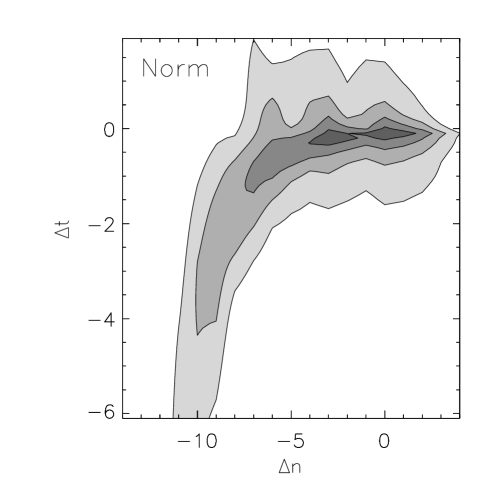
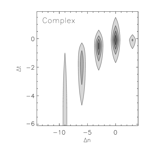
Figure 2: The two-point correlation in shells and time first for the norm of the amplitudes and second for the pure amplitudes, based at the 15’th shell.

The left plot show that all the amplitudes in the model is strongly correlated from the forcing at the $4^{\textrm{th}}$ shell up to the highest shells. This strong correlation is due to the organisation of the amplitude dynamics during both bursts and the succeeding strong oscillations. The same plot also shows the motion of the burst through the shells by the time-shift of the correlation-peeks for increasing $\Delta n$. When taking the amplitude phases into account the correlation function changes radically as seen in the right plot. Now only every third amplitude are correlated and this comes as a result of the period three invariance of the model. This plot shows also how the characteristic time-scale changes among the different shells. It is seen by the extent of the correlation-peeks in time which decreases with shell-number. When relating the characteristic time-scale to the turnover-time ($\tau_{n}$) this dependence comes direct from dimension analysis [1].

3.2 Front motion during burst

The motion of the bursts is a part of a more general motion of different organisations of the amplitudes travelling with exponential increasing speed from the lower towards the higher shells where they vanish because of viscosity [10]. A way to see this is to look at the changes in the instantaneous amplitude spectre during the motion of a burst. This is shown in Fig.3 by snapshots of $\ln|u_{n}(t)|$ vs. $n$ where the time between snapshots decrease by a factor of $1/\sqrt{2}$ giving roughly an equidistant motion of the burst. As for all other bursts Fig.3 reveals that the burst travels through the shells as a front keeping the same overall shape. Just at the maximum rise of the amplitudes the overall scaling exponent of the inertial range is a bit lower than the Kolmogorov scaling-law shown by the dashed line in Fig.3. Immediately after the last snapshot all the shells enters the oscillatory state.

Figure 3: Snapshots of $\log|u_{n}|$ during the cascade of a burst

3.3 Real-valued model

Due to the invariance in the model the creation and behaviour of the bursts are unaffected by the complex phase of the amplitudes. A model in terms of real values will therefore be used in the following analysis:

$$\left({d\over dt}+\nu k_{n}^{2}\right)r_{n}=-k_{n}(r_{n+1}r_{n+2}-\frac{1}{4}r_{n-1}r_{n+1}-\frac{1}{8}r_{n-2}r_{n-1})+f\delta_{n,4}$$ (4)

having $r_{n}=|u_{n}|$, no conjugations and “$-1$” instead of “$i$” in front of the coupling-term [11].

4 Local variables

From the construction of the model the dynamics of a given shell depends only on the instantaneous configuration of the neighbouring shells and it has no explicit dependence on the present or past states. If we at first restrict ourself to the inertial range neglecting forcing and viscosity the neighbouring shells may be seen as a local phase-space of a shell since their configuration through the coupling-term exactly determines the instantaneous dynamics $(\dot{r}_{n})$ of the amplitude $r_{n}$. To characterise this local phase-space each set of neighbouring shells will be called the local shells: $\vec{L}_{n}=(r_{n-2},r_{n-1},r_{n+1},r_{n+2})$ of the n${}^{\textrm{th}}$ shell, and they should not be seen as part of the other amplitudes but rather as an isolated set of variables determining $\dot{r}_{n}$.
The configuration of $\vec{L}_{n}$ will be described by first choosing the slope of $\ln_{\lambda}(\vec{L}_{n})$ which is nothing but the local scaling exponent at the n${}^{\textrm{th}}$ shell. To continue we define

$$\vec{\eta}_{n}\equiv\ln_{\lambda}(\vec{L}_{n})$$ (5)

and choose the mean, curvature and third order component of $\vec{\eta}_{n}$. This gives the local variables: $\vec{P}_{n}=(A_{n},\,B_{n},\,C_{n},\,D_{n})$ of $r_{n}$ defined as the coefficients of the projection of $\vec{\eta}_{n}$ on the orthogonal basis given by the matrix $\mathbf{T}$ :

$$\vec{\eta}_{n}=\mathbf{T}\cdot\vec{P}_{n},\quad\vec{L}_{n}=2^{\vec{\eta}_{n}}$$ (6)

where

$$\mathbf{T}=\left(\begin{array}[]{cccc}\alpha&2\beta&-\alpha&\beta\\ \alpha&\beta&\alpha&-2\beta\\ \alpha&-\beta&\alpha&2\beta\\ \alpha&-2\beta&-\alpha&-\beta\end{array}\right)$$ (7)

and $\alpha=1/4$ and $\beta=1/10$.
The basis of the local variables is plotted in Fig.4 showing how it can be characterised as a simple “Taylor-series” expansion of $\vec{\eta}_{n}$. These variables are believed to be the right variables to monitor the dynamics of the model since they describe globally the configuration of the local shells instead of focusing on the individual neighbouring shells. The local scaling of shell-models has been studied earlier [9, 8], but this was the instantaneous local scaling averaged over all shells and using a coarse-grained time resolution.

Figure 4: The basis of the local variables

4.1 Application to the model

To implement Eq.6,7 into the model we assume the components of $\vec{\eta}_{n}$ to behave smoothly in $n$ such that $r_{n}\approx 2^{A_{n}}$, giving:

$$\dot{r}_{n}=-\,k_{n}\,2^{2A_{n}}\left(2^{3B_{n}-D_{n}}-\mbox{$\delta\over 2$}2^{-2C_{n}}-\mbox{${1-\delta}\over 4$}2^{-3B_{n}+D_{n}}\right)-\nu\,k_{n}^{2}\,2^{A_{n}}.$$ (8)

Eq.8 gives direct evidence of the period three invariance of the model: Since the dynamics only depends on the combinations ($3B_{n}-D_{n},\,C_{n},\,A_{n}$), we define $E_{n}\equiv 3B_{n}-D_{n}$. The model is then invariant to the orthogonal component of $E_{n}$: $\perp\!E_{n}=3D_{n}+B_{n}$ which is nothing but the period three invariance as seen in in Fig.5.

Figure 5: The period three invariance of the local basis

From the construction of Eq.8 is should be noted that the sign of $\dot{r}_{n}$ and thereby the monotony of the dynamics is only a function of $E_{n}$ and $C_{n}$ when neglecting the viscosity-term. Because $A_{n}$ is outside the brackets it will affect the response-time of the dynamics. Now the dynamics of the n${}^{\textrm{th}}$ amplitude is only determined by three local variables:

$$\vec{V}_{n}=(E_{n},\,C_{n},\,A_{n}).$$

Even though this new set of local variables ($\vec{V}_{n}$) form a efficient phase-space it should not be confused with the actual 2N-dimensional phase-space of the free variables in the model.

4.2 The Local Attractor of the model

Since $\vec{V}_{n}$ is a local phase-space the trajectory of $\vec{V}_{n}(t)$ in time will describe a three dimensional local attractor of the n${}^{\textrm{th}}$ shell dynamics. Fig.6 show the local attractor of the 14${}^{\textrm{th}}$ shell during a time-span of two successive bursts where some additional features is placed to explain the dynamics of the attractor:

Figure 6: The local attractor of the 14’th shell and its projection on a $(E_{n},C_{n})$-plane together with the surface of $\dot{r}_{n}=0$, the Kolmogorov fixed-point-line and arrows of characteristic flow.

First we note that the trajectory is projected down on a $(E_{n},C_{n})$-plane to help giving a three dimensional understanding of the attractor. Then we focus on the vertical line which correspond to the Kolmogorov fixed-point given by $(E_{n},C_{n},A_{N})=(-1,0,\cdot)$. Right after every bursts the trajectories encircles this line during the relaxations. As the oscillations die out the dynamics slow down making the trajectories stay close to the region of $\dot{r}_{n}\approx 0$ in $\vec{V}_{n}$. In Fig.6 the curved sheet is the manifold of $\dot{r}_{n}=0$ derived from Eq.8 and it is seen how the trajectory stays close to the manifold. ( note that the trajectory is shown thinner for negative $\dot{r}_{n}$)
When a burst approaches from the lower shells it affects the configuration of local shells forcing the trajectory away from the manifold. This causes $\dot{r}_{n}$ and thereby $r_{n}$ to increase rapidly making the shell participate the burst. During the burst the trajectory approaches the Kolmogorov fixed-point-line around which it begins to circle again etc. The same behaviour repeats throughout the evolution of the model making the local attractor capture all the general dynamics of the model.
Every other shell participating in the burst has qualitatively the same local attractor with the same characteristics. It should be noted that if the viscous term only affects the last shells, abandoning the inertial range, the model would still produce bursts and in this case the oscillations would not bend off but follow the Kolmogorov fixed-point strait down until the next burst approaches.

5 The cause of intermittency

From the behaviour of the local attractor it is possible to explain the intermittent shift between bursts and oscillatory relaxation of the model. What is needed is the answers to the following two questions: Why is the manifold of $\dot{r}_{n}=0$ stable, attracting the oscillatory state into a relaxing period and what changes this stability as a burst approaches.

5.1 Creation of the relaxing period.

To analyse the stability of the manifold we have to know the flow in the phase-space $\vec{V}_{n}$ and this will be done by estimating $\dot{A}_{n},\dot{E}_{n},\dot{C}_{n}$:
First we assume again $r_{n}\approx 2^{A_{n}}$ to get $\dot{r}_{n}\approx\ln(2)\,2^{A_{n}}\dot{A}_{n}$ which will be used to estimate $\dot{A}_{n}$. Then we insert $\dot{A}_{n}$ into the transformations of Eq.6 getting $\dot{E}_{n}$ and $\dot{C}_{n}$ as a function of $\dot{A}_{n+j},\ j=\{-2,1-,1,2\}$. To proceed we note that because of the regular dynamics during oscillations all the local variables for the different shells are roughly equal despite a Kolmogorov-scaling of the mean values ($A_{n}$). This makes us assume the following condition between the local variables:

$$\left(A_{n+j},E_{n+j},C_{n+j}\right)\approx\left(A_{n}-\mbox{$j\over 3$},E_{n},C_{n}\right),\ j=\{-2,1-,1,2\}$$ (9)

When inserted into the different $\dot{A}_{n+j}$ it causes $\dot{E}_{n}$ and $\dot{C}_{n}$ to resemble $\dot{A}_{n}$ within pre-factors in front of the coupling- and viscous-terms.
As result the monotony of $\dot{E}_{n}$ and $\dot{C}_{n}$ follows that of $\dot{A}_{n}$.
Now the general flow in $\vec{V}_{n}$ only depends on the sign of $\dot{r}_{n}$, changing at the manifold and indicated by the arrows showed in Fig.6. From the orientation of the flow and the position of the manifold the trajectory is caused to close in on the manifold and slowly drift downwards creating a relaxing period.

5.2 Bursts

The stability of the manifold and thereby of the relaxing state depends critically on the condition of Eq.9 used in the derivation above. The thing that destroys this condition is the approach of a burst from the lower shells, affecting only $r_{n-2},r_{n-1}$. The manifold then loses its stability and the state is forced into a region of strong positive $\dot{r}_{n}$ making the shell participate in the burst. Now as $r_{n}$ changes violently it causes the manifold of the higher shells to become unstable etc. and thus the burst spreads through the shells because of a chain-reaction.

6 Conclusion

In this article the standard GOY shell model has been analysed on the basis of its dynamics rather than its statistics. A detailed analysis of the time-evolution revels the following:
The dynamics of the model follows two different states where violent bursts are interchanged by an oscillatory relaxing state. It is showed that the dynamics of the shells are mutually correlated and the burst travels through the shells like a front. Because bursts in the model cascade nearly unaffected through the shells in the inertial range, each set of neighbouring shells entering the coupling-terms can be seen as local phase-spaces of the corresponding shells, and when expressed in a simple “Taylor-series” base their dynamics describe an approximative attractor of the model. From the dynamics of the local attractor the intermittency of the model is explained.

6.1 Acknowledgements

I would like to thank the following people for fruitful discussions concerning this work: Ken Haste Andersen, Jacob Sparre Andersen, Tomas Bohr, Jesper Borg, Paolo Muratore Ginanneschi, Martin van Hecke, Anders Johansen, Jens Juul Rasmussen, Bjarne Stenum and my supervisor Mogens Høgh Jensen.

References

- [1] U. Frisch, ”Turbulence: The legacy of A. N. Kolmogorov”, Cambridge University Press (1995).
- [2] A. N. Kolmogorov, C. R. Acad. Sci. USSR 30, 301; ibid 32, 16 (1941).
- [3] F. Belin, J. Maurer, P. Tabeling and H. Willaime, “Observation of worms between counter rotating cylinders”, , J. Phys II France, 6, 1-19 (1996).
- [4] E. B. Gledzer, Sov. Phys. Dokl. 18, 216 (1973).
-
[5]
M. Yamada and K. Ohkitani, J. Phys. Soc. Japan 56, 4210
(1987)
Prog. Theor. Phys. 79,1265 (1988). - [6] M. H. Jensen, G. Paladin and A. Vulpiani, Phys. Rev. A 43, 798 (1991).
- [7] L. Kadano, D. Lohse, J. Wang and R. Benzi, Phys. Fluids 7, 617 (1995).
- [8] T. Bohr, M. H. Jensen, G. Paladin and A. Vulpiani, Dynamical systems approach to turbulence, Cambridge University Press, Cambridge (1998).
- [9] L. Biferale, A. Lambert, R. Lima and G. Paladin. Physica D 80, 105 (1995).
- [10] T. Dombre and J.-L. Gilson, “Intermittency, chaos and singular fluctuations in the mixed Obukhov-Novikov shell model of turbulence”, Preprint (1996).
-
[11]
F. Okkels, Master thesis, CATS, University of Copenhagen,
Denmark (1997).
F. Okkels and M. H. Jensen, Phys. Rev. E, 57, n.6, 6643 (1998).