The Control of Dynamical Systems
– Recovering Order from Chaos –

Abstract

Following a brief historical introduction of the notions of chaos in dynamical systems, we will present recent developments that attempt to profit from the rich structure and complexity of the chaotic dynamics. In particular, we will demonstrate the ability to control chaos in realistic complex environments. Several applications will serve to illustrate the theory and to highlight its advantages and weaknesses. The presentation will end with a survey of possible generalizations and extensions of the basic formalism as well as a discussion of applications outside the field of the physical sciences. Future research avenues in this rapidly growing field will also be addressed.

Abstract

Following a brief historical introduction of the notions of chaos in dynamical systems, we will present recent developments that attempt to profit from the rich structure and complexity of the chaotic dynamics. In particular, we will demonstrate the ability to control chaos in realistic complex environments. Several applications will serve to illustrate the theory and to highlight its advantages and weaknesses. The presentation will end with a survey of possible generalizations and extensions of the basic formalism as well as a discussion of applications outside the field of the physical sciences. Future research avenues in this rapidly growing field will also be addressed.

– Octobre 1999 –

Invited Talk at the XXIth International Conference on the Physics of Electronic and Atomic Collisions (ICPEAC), July 22-27, 1999 (Sendai, Japan).
 
in The Physics of Electronic and Atomic Collisions, ed. Y. Itikawa, AIP Conference Proceedings 500, 551-570 (2000) (AIP: Woodbury, N.Y.)

The Control of Dynamical Systems
– Recovering Order from Chaos –

Louis J. Dubé and Philippe Després

Introduction

In his 1985 Gifford Lectures, Freeman Dyson expressed his opinion on the matter of chaos. In his subsequently published words DYS88 , the chapter entitled “Engineers’ Dreams” contains the following statement:

A chaotic motion is generally neither predictable nor controllable. It is unpredictable because a small disturbance will produce exponentially growing perturbation of the motion. It is uncontrollable because small disturbances lead only to other chaotic motions and not to any stable and predictable alternative. Von Neumann’s mistake was to imagine that every unstable motion could be nudged into a stable motion by small pushes and pulls applied at the right places.

As one can see, the assertion was also meant as an answer to comments made by von Neumann in the early 1950s and who obviously held a less pessimistic point of view. Dyson’s position represents well the traditional wisdom until 1990 …

In order to appreciate why the juxtaposition of the two words chaos and control is so counter-intuitive and why Dyson’s statement was so representative and sensible, an operational definition of chaos will be helpful. In our exposition, the word chaos has a technical and precise meaning to be distinguished from its greek origin where it designated “the primeval emptiness of the universe before things came into being of the abyss of Tartarus, the underworld” . A universal definition is not available, but most researchers would agree that deterministic chaos could be described as follows:
Chaos is a long-term aperiodic behaviour of a dynamical system that possesses the property of sensitivity to initial conditions.
– long-term aperiodic behaviour means that the time evolution of the system does not tend towards a stationary or periodic state, i.e. regularity of the motion is absent.
– dynamical system describes a process whose future behaviour is strictly determined by its past state, i.e. determinism is present and the source of the irregularity is inherent and not to be found in a stochastic component.
– sensitivity to initial conditions implies that a very small deviation in the initial conditions is sufficient to create large deviations in the future states (the so-called “butterfly effect”), i.e. despite the presence of determinism, practical long-term predictability is lost.

This is the type of motion that Dyson had in mind. It is not new of course and it is clear that Maxwell and Boltzmann, the founders of statistical physics, were acutely aware of the property of sensitivity to initial conditions and its consequences. Not before Poincaré POI1890 however, could one ascertain the existence of this property in a system with few degrees of freedom, namely the reduced 3-body problem. In the continuing history of nonlinear dynamical systems, the first evidence of physical chaos is associated with the name of Edward Lorenz LOR63 , whose 1963 discovery of the first strange attractor in a simplified meteorological model containing only 3 state variables has led to a remarkable explosion in the study of chaos and its properties. It was not until 1990 however that Ott, Grebogi and Yorke (OGY) OTT90 addressed the question of control of chaos and described, very much in the spirit of von Neumann, the theoretical steps necessary to achieve this goal. This work was rapidly followed by experimental verification DIT90 : von Neumann’s dream had become reality.

This Progress Report will describe some practical implementations for the recovery of order from chaos. The theoretical foundations of the methods will be first explained for 1D and 2D systems and then demonstrated with some recent calculations taken from mathematics and physics. Our conclusions and a glimpse at future applications and extensions make the last part of the presentation. Lack of space precludes completeness, and the interested reader may wish to consult the special 1997 Decembre issue of Chaos for further information.

The Control Strategy

All stable processes, we shall predict.
All unstable processes, we shall control.
John von Neumann, circa 1950

In this Section, we show how the richness, the complexity and the sensitivity of chaotic dynamics can be used to select and stabilize at will, with small programmed perturbations, an otherwise unstable state of the natural dynamics. The goal is to achieve this feat without altering appreciably the original system. It is precisely the properties that differentiate a chaotic motion from an irregular or unstable behaviour that are the solution to the control task. The important ingredients are:
– unstable periodic orbits (UPO) are typically dense in the chaotic attractor of dissipative systems or in the stochastic web of conservative systems, i.e. there are practically an infinity of unstable states to choose from.
– chaotic motion is ergodic, meaning that a chaotic trajectory will revisit infinitely often the neighbourhood of any point within the available phase space.
– chaotic dynamics is sensitive to initial conditions, implying that small perturbations will naturally induce large effects.

To go beyond qualitative description, we establish some working conditions:

1. we suppose that the dynamics can be represented by a $d$-dimensional nonlinear map (either given explicitly or reconstructed from the observations)

   $${\bf x}_{n+1}={\mathbf{F}}({\bf x}_{n},p)$$ (1)

   where $p$ is an accessible system parameter, the control parameter.

2. there exists one or more specific UPOs for a given nominal value $p_{0}$ of the parameter, defined by

   $$\{{\bf x}(i,p_{0}):{\bf x}(i,p_{0})={\mathbf{F}}^{(m)}({\bf x}(i,p_{0}),p_{0})\ ,\qquad\forall\ i=1,m\}$$ (2)

   for an orbit of period $m$, around which one wishes to stabilize the dynamics.

3. control is activated only when points of the trajectory $\{{\bf x}_{n}\}$ fall in a small neighbourhood of the UPOs, usually taken to be a ball ${\cal B}_{\delta}$ of radius $\delta$ around $\{{\bf x}(i,p_{0})\}$ ,

   $$|{\bf x}_{n}-{\bf x}(i,p_{0})|\leq\delta\qquad\qquad\mbox{for some}\quad i=1,m\quad,$$ (3)

   hereafter referred to as the control or $\delta-$neighbourhood.

4. we restrict the parameter variations $\delta p$, necessary to achieve control, to a maximum small perturbation

   $$|\delta p|\leq|\delta p_{\rm max}|\ll|p|$$ (4)

   defining the control range.

5. since the position of a periodic orbit is a function of $p$, and we assume that the local dynamics does not vary much within $|\delta p|$, a linear representation of the dynamics is possible.

Obviously, the control range and neighbourhood are not independent and experience shows that a judicious choice is to take them of the same order of magnitude.

1D Control

In a 1D system where the nonlinear map is given explicitly by

$$x_{n+1}=F(x_{n},p)\quad,$$ (5)

and where a target UPO of period $m$, i.e. $\{x(i,p_{0})\}$, exists at nominal value $p_{0}$ of the control parameter, the perturbations necessary to stabilize the orbit can be calculated directly. Indeed, assume that at the $n$-th iteration, $x_{n}$ comes in ${\cal B}_{\delta}$ of the $i$-th component of the target UPO, i.e. $|x_{n}-x(i,p_{0})|\leq\delta$, then equation (5) can easily be linearized around $x(i,p_{0})$ and $p=p_{0}$ such that

$$x_{n+1}-x(i+1,p_{0})\sim U_{i}\ [x_{n}-x(i,p_{0})]+V_{i}\ [p_{n}-p_{0}]\equiv U_{i}\ \delta x_{n,i}+V_{i}\ \delta p_{n}$$ (6)

where $U$ is the Jacobian of the map and $V$ expresses the parametric variation of the map

$$U=D_{x}F(x,p)=\frac{\partial}{\partial x}F(x,p)\qquad V=D_{p}F(x,p)=\frac{\partial}{\partial p}F(x,p)\quad.$$ (7)

The notation $U_{i}$ and $V_{i}$ indicates that the partial derivatives are evaluated at $[x=x(i,p_{0}),p=p_{0}]$. To obtain an expression for $\delta p_{n}$, one imposes the control criterion (not unique) that equation (6), taken as a strict equality, should be equal to zero, namely that

$$x_{n+1}-x(i+1,p_{0})=0\quad.$$ (8)

(control criterion 1D)   
Solving for $\delta p_{n}$, equation (6) leads immediately to

$$\delta p_{n}=-\frac{U_{i}}{V_{i}}\ \delta x_{n,i}\quad.$$ (9)

In order to complete the procedure, one should make sure that $|\delta p_{n}|$ just obtained is $\leq\delta p_{\rm max}$ (we will always take $\delta p_{\rm max}>0$ ). If it is so, $p_{n}=p_{0}+\delta p_{n}$ for the next iteration; if not, one could set $p_{n}=p_{0}$ and wait until the trajectory reenters ${\cal B}_{\delta}$. We have found that a more robust choice is to apply the corrections during the control stage according to the prescription

$$\delta p_{n}\longrightarrow\delta p_{\rm max}\tanh(\delta p_{n}/\delta p_{\rm max})\qquad{\rm for}\qquad|\delta p_{n}|>\delta p_{\rm max}\quad.$$ (10)

This is a minor point however since typically $\delta p_{n}$ decreases rapidly after the first few iterations as we are getting ever closer to the target orbit ($\delta p_{n}\propto\delta x_{n}$).

2D Control

Stabilization in higher dimensions is qualitatively different from the 1D case since phase space is endowed with a much richer structure. For simplicity, we will confine our discussion to two dimensions. In 2D, the generic local neighbourhood of a UPO is equipped with a stable and unstable manifold. A chaotic trajectory entering the neighbourhood will move toward the UPO along the stable direction and escape along the unstable one. This is the “saddle dynamics” illustrated in Figure (1).

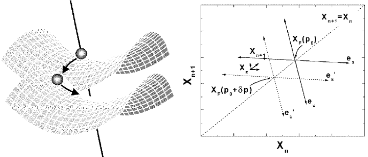
Figure 1: Local Geometry of Control: (left) 2D “saddle dynamics” and (right) linearization of the stable and unstable manifolds.

OGY OTT90 realized that a possible solution of controlling chaos could be obtained by locally displacing the manifolds such that the component of the motion along the unstable direction could be eliminated (at least to first order) such that subsequent evolution will naturally lead the orbit to the unstable point along the stable direction. This idea is geometrically presented in Figure (1) for the situation of an unstable fixed point denoted ${\bf x}_{F}(p_{0})$, much like the task of bringing a ball bearing to rest on a saddle. The remaining part of this subsection is devoted to the mathematical translation of the applications of “small pushes and pulls applied at the right places”.

Starting from the 2D nonlinear map

$${\bf x}_{n+1}={\mathbf{F}}({\bf x}_{n},p)$$ (11)

with ${\bf x}_{n}\in{\cal R}^{2}$ and $p\in{\cal R}$, one traces the steps to achieve control through the following algorithm.

1. locate a UPO of period $m$ for the nominal value of the parameter $p_{0}$

   $${\bf x}(1,p_{0})\to{\bf x}(2,p_{0})\to\cdots{\bf x}(m,p_{0})\to{\bf x}(m+1,p_{0})={\bf x}(1,p_{0})\quad.$$ (12)

2. linearize the dynamics in the $\delta$-neighbourhood of ${\bf x}(i,p_{0})$ :

   $${\bf x}_{n+1}-{\bf x}(i+1,p_{0})\sim{\bf U}_{i}\ \left[{\bf x}_{n}-{\bf x}(i,p_{0})\right]+{\mathbf{V}}_{i}\ \delta p_{n}$$ (13)

   where ${\bf U}$ is the $2\times 2$ Jacobian matrix and ${\mathbf{V}}$ is a $2\times 1$ parametric variation vector

   $${\bf U}\equiv D_{{\bf x}}\ {\mathbf{F}}({\bf x},p)\qquad{\rm and}\qquad{\mathbf{V}}\equiv D_{p}\ {\mathbf{F}}({\bf x},p)$$ (14)

   with the partial derivatives evaluated at $[{\bf x}={\bf x}(i,p_{0}),\ p=p_{0}]$.

3. characterize the local dynamics by the stable ${\mathbf{e}}_{s,i}$ and the unstable ${\mathbf{e}}_{u,i}$ directions.

4. construct the contravariant vectors defined by

   $${\mathbf{f}}_{u,i}\cdot{\mathbf{e}}_{u,i}={\mathbf{f}}_{s,i}\cdot{\mathbf{e}}_{s,i}=1\qquad\qquad{\mathbf{f}}_{u,i}\cdot{\mathbf{e}}_{s,i}={\mathbf{f}}_{s,i}\cdot{\mathbf{e}}_{u,i}=0\quad.$$ (15)

5. stabilize the orbit by demanding that it falls, on the next iteration, on the stable direction, i.e.

   $${\mathbf{f}}_{u,i+1}\cdot\left[{\bf x}_{n+1}-{\bf x}(i+1,p_{0})\right]=0\quad.$$ (16)

   (control criterion OGY)   
   Therefore, according to step 2, we obtain the relation

   $${\mathbf{f}}_{u,i+1}\cdot\left\{{\bf U}_{i}\ \left[{\bf x}_{n}-{\bf x}(i,p_{0})\right]+{\mathbf{V}}_{i}\ \delta p_{n}\right\}=0\quad.$$ (17)

6. calculate the perturbation necessary to satisfy equation (17)

   $$\delta p_{n}=-\ \frac{{\mathbf{f}}_{u,i+1}\cdot\left\{{\bf U}_{i}\ \left[{\bf x}_{n}-{\bf x}(i,p_{0})\right]\right\}}{{\mathbf{f}}_{u,i+1}\cdot{\mathbf{V}}_{i}}$$ (18)

   and apply only if $|\delta p_{n}|<\delta p_{\rm max}$ otherwise set e.g. $\delta p_{n}=0$ or use equation (10).

In summary, the stabilization procedure can be divided in three separate stages: the learning stage, where one identifies the desired UPOs, extracts the Jacobian matrices, and calculates the corresponding stable and unstable directions ${\mathbf{e}}_{s,i}$ , ${\mathbf{e}}_{u,i}$ to construct the contravariant vectors ${\mathbf{f}}_{u,i}$ ; the transient stage, where, after randomly choosing an initial condition, the system is let to evolve freely at the nominal parameter value $p_{0}$ until, at the control stage, once the chaotic trajectory has entered the prescribed $\delta$-neighbourhood, the control is attempted by means of small parameter perturbations.

Alternative Control Algorithms

The algorithm just described is dynamically optimal in that it uses a control criterion and perturbations that involve the complete local structure of the system’s dynamics. From a practical (experimental) point of view, it is also most demanding considering that the underlying dynamical law is often not even known a priori. It requires the determination of the Jacobian matrices and the parametric variation of the map along the UPOs and the corresponding stable and unstable directions. Several modifications of the original method have been proposed and we now present some of them with an emphasis towards algorithms that are simpler and in some instances more practicable.

If instead of equation (13), one writes the linearization as

$${\bf x}_{n+1}-{\bf x}(i+1,p_{n})\sim{\bf U}_{i}\ \left[{\bf x}_{n}-{\bf x}(i,p_{n})\right]$$ (19)

where the dependence of ${\mathbf{U}}_{i}$ on $p$ has been ignored, and one introduces the parametric variation of the periodic points as

$${\bf g}_{i}\equiv\left.\frac{d}{dp}\ {\bf x}(i,p)\right|_{p=p_{0}}\sim\frac{{\bf x}(i,p_{0}+\delta p)-{\bf x}(i,p_{0})}{\delta p}$$ (20)

or equivalently,

$${\bf x}(i,p_{0}+\delta p)\sim{\bf x}(i,p_{0})+{\mathbf{g}}_{i}\ \delta p\quad,$$ (21)

one arrives, under the criterion (16), to the perturbations

$$\delta p_{n}=-\ \frac{{\mathbf{f}}_{u,i+1}\cdot\left\{{\bf U}_{i}\ \left[{\bf x}_{n}-{\bf x}(i,p_{0})\right]\right\}}{{\mathbf{f}}_{u,i+1}\cdot({\mathbf{g}}_{i+1}-{\mathbf{U}}_{i}\ {\mathbf{g}}_{i})}\quad.$$ (22)

The expression (22) has the advantage that the variables ${\mathbf{g}}_{i}$ can easily be obtained from observations of the shift of the periodic points under small parameter change.

One further simplification arises if it is sufficient to intervene on the dynamics only once per period. The modifications to the formula are straightforward. Equation (19) becomes

$${\bf x}_{n+m}-{\bf x}_{F,i}(p_{n})\sim{\bf U}_{i}^{(m)}\ \left[{\bf x}_{n}-{\bf x}_{F,i}(p_{n})\right]$$ (23)

where the notation is chosen to emphasize that ${\bf x}_{F,i}(p)={\bf x}(i,p)$ is a fixed point of ${\mathbf{F}}^{(m)}$ (the $m$ times application of the map ${\mathbf{F}}$). Furthermore, the Jacobian matrix ${\bf U}_{i}^{(m)}=D_{{\bf x}}{\mathbf{F}}^{(m)}({\bf x},p)$, evaluated at $[{\bf x}_{F,i}(p_{0}),p_{0}]$, can be expanded in terms of its eigenvectors (the stable and unstable manifolds) and eigenvalues as $\lambda_{u,i}\ {\mathbf{e}}_{u,i}{\mathbf{f}}_{u,i}+\lambda_{s,i}\ {\mathbf{e}}_{s,i}{\mathbf{f}}_{s,i}$ to modify (22) to

$$\delta p_{n}=-\ \frac{\lambda_{u,i}}{(1-\lambda_{u,i})}\frac{{\mathbf{f}}_{u,i}\cdot\left[{\bf x}_{n}-{\bf x}_{F,i}(p_{0})\right]}{{\mathbf{f}}_{u,i}\cdot{\mathbf{g}}_{i}}\quad.$$ (24)

Until now the control criterion has not been modified, but in situations where the stable and unstable manifolds may be difficult to obtain (e.g. in high dimensions) or for the sake of simplicity, one might choose to minimize the deviation from the target orbit instead of projecting onto the stable manifold, i.e. we demand that

$$||{\bf x}_{n+m}-{\bf x}_{F,i}||={\rm minimum}\quad,$$ (25)

(control criterion MED)   
where an estimate of ${\bf x}_{n+m}$ is given by equations (23) and (21), namely

$${\bf x}_{n+m}\sim{\bf x}_{F,i}(p_{0})+{\bf U}_{i}^{(m)}\ \left[{\bf x}_{n}-{\bf x}_{F,i}(p_{0})\right]+({\mathbf{g}}_{i}-{\mathbf{U}}_{i}^{(m)}\ {\mathbf{g}}_{i})\ \delta p_{n}\quad.$$ (26)

The solution of the minimization (25) is then

$$\delta p_{n}=-\ \frac{({\mathbf{g}}_{i}-{\mathbf{U}}_{i}^{(m)}\ {\mathbf{g}}_{i})\cdot\left\{{\bf U}_{i}^{(m)}\ \left[{\bf x}_{n}-{\bf x}_{F,i}(p_{0})\right]\right\}}{||({\mathbf{g}}_{i}-{\mathbf{U}}_{i}^{(m)}\ {\mathbf{g}}_{i})||^{2}}\quad.$$ (27)

This technique was first introduced in REY93 and goes by the name of minimal expected deviation (MED) method.

The perturbations $\delta p_{n}$ transform the original autonomous systems to nonautonomous ones. One could therefore consider a formulation extending phase space by one dimension with $p_{n}$ as the new dynamical variable. Alternatively, as was first realized in DRE92 , one could account explicitly for the $p_{n}$ dependence by introducing in the mapping itself the past history of the perturbations, namely

$${\bf x}_{n+1}={\mathbf{F}}_{c}({\bf x}_{n},p_{n},p_{n-1})\quad.$$ (28)

We restrict ourselves to the last two perturbations. The sub-index on ${\mathbf{F}}_{c}$ is to remind us that the mapping differs from the original one and is only identical to it when $p_{n}=p_{n-1}=p_{0}$. In analogy to equation (26), one can write

$${\bf x}_{n+m} \sim {\bf x}_{F,i}(p_{0},p_{0})+{\bf U}_{i}^{(m)}\ \left[{\bf x}_{n}-{\bf x}_{F,i}(p_{0},p_{0})\right]$$ (29)

$$+({\mathbf{g}}_{u,i}-{\mathbf{U}}_{i}^{(m)}\ {\mathbf{g}}_{u,i})\ \delta p_{n}+({\mathbf{g}}_{b,i}-{\mathbf{U}}_{i}^{(m)}\ {\mathbf{g}}_{b,i})\ \delta p_{n-1}\quad.$$

with

$${\mathbf{g}}_{u}=\left.\frac{d}{dp}\ {\bf x}_{F}(p,p^{\prime})\right|_{p=p^{\prime}=p_{0}}\qquad\qquad{\mathbf{g}}_{b}=\left.\frac{d}{dp^{\prime}}\ {\bf x}_{F}(p,p^{\prime})\right|_{p=p^{\prime}=p_{0}}\quad.$$ (30)

To complete the modification, a control condition must be imposed and a reasonable choice is

$$[{\bf x}_{n+2m}-{\bf x}_{F,i}(p_{0},p_{0})]=0\qquad{\rm and}\qquad\delta p_{n+1}=0\quad.$$ (31)

(control criterion RPF)    
The conditions (31) are sufficient to solve the linearized equation (29) for $\delta p_{n}$ as

$$\delta p_{n}=-\ \frac{{\mathbf{X}}_{i}^{(m)}\cdot\{{\mathbf{U}}_{i}^{(m)}\ {\mathbf{U}}_{i}^{(m)}\ [{\bf x}_{n}-{\bf x}_{F,i}(p_{0},p_{0})]\}}{||{\mathbf{X}}_{i}^{(m)}||^{2}}-\ \frac{{\mathbf{X}}_{i}^{(m)}\cdot({\mathbf{U}}_{i}^{(m)}\ {\mathbf{W}}_{i}^{(m)})}{||{\mathbf{X}}_{i}^{(m)}||^{2}}\ \delta p_{n-1}$$ (32)

with ${\mathbf{X}}_{i}^{(m)}={\mathbf{U}}_{i}^{(m)}\ {\mathbf{V}}_{i}^{(m)}+{\mathbf{W}}_{i}^{(m)}$, ${\mathbf{V}}_{i}^{(m)}={\mathbf{g}}_{u,i}-{\mathbf{U}}_{i}^{(m)}\ {\mathbf{g}}_{u,i}$ and ${\mathbf{W}}_{i}^{(m)}={\mathbf{g}}_{b,i}-{\mathbf{U}}_{i}^{(m)}\ {\mathbf{g}}_{b,i}$. Our derivation is somewhat different from ROL93 and , in view of the numerous parameters to determine, it should be taken as a serious alternative only for 1D (or quasi 1D) systems. In the latter case, the method has a simple geometrical interpretation as illustrated in the right panel of Figure (2) for an unstable fixed point $x_{F}(p_{0})$: $U$ is the local slope of the original map, $g_{u}\delta p$ and $g_{b}\delta p$ correspond to the shifts of the fixed point to positions $x_{F,u}(p_{0}+\delta p,p_{0})\sim x_{F}(p_{0})+g_{u}\delta p$ and $x_{F,b}(p_{0},p_{0}+\delta p)\sim x_{F}(p_{0})+g_{b}\delta p$ respectively, whereas $V\delta p$ denotes the map displacement from $F_{c}(x,p_{0},p_{0})\equiv F(x,p_{0})\to F_{u}(x,p_{0}+\delta p,p_{0})$ and $W\delta p$ from $F(x,p_{0})\to F_{b}(x,p_{0},p_{0}+\delta p)$. These parameters are readily obtained from the observations as was first demonstrated by ROL93 who gave the algorithm the name of recursive proportional feedback (RPF).

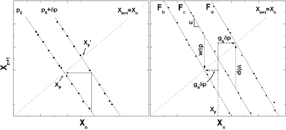
Figure 2: Alternative Local Geometries of Control: (left) the Occasional Proportional Feedback (OPF) method and (right) the Recursive Proportional Feedback (RPF) method.

Our last modification, which we only quote for 1D systems where it is most likely to be used, consists of ignoring in the RPF formula the dependence on $p_{n-1}$ which amounts to setting $W=0$ in the previous equations, to obtain

$$\delta p_{n}=-\ \frac{U}{(g-U\ g)}\ [x_{n}-x_{F,i}(p_{0})]\quad.$$ (33)

One should not be deceived by the apparent simplicity of equation (33). In its regime of applicability, it can be enormously successful as we will see shortly and as Hunt HUN91 first demonstrated. Its geometrical interpretation is shown in the left panel of Figure (2) where it amounts to choose a perturbation such that upon the next iteration, $x_{n}$ is mapped onto the target fixed point. This occasional proportional feedback (OPF), as it was called originally, is eminently suited for experimental control since it requires feedback signals proportional to the deviations to the target orbit and two parameters $U$ and $g$ readily available. Even more, if one is bold enough, one might just as well adjust the proportionality constant until control is established.

Mathematical and Physical Applications

We have selected five examples of increasing complexity and novelty. The first three correspond to dissipative systems confined to a chaotic attractor, whereas the last two are conservative Hamiltonian systems where the attractor is replaced by bounded regions of phase space where the dynamics is chaotic.

We will apply the perturbations only once per period for all cases except the last. Save for the two discrete maps, ALL the relevant control informations are obtained numerically in an effort to simulate more closely an experimental setting. Reliable methods (see e.g. OTT94 ) exist to locate the positions of the UPOs and we will assume thereafter that the locations are known prior to the control session. The numerical construction of the Jacobian matrices from time series is often a subtle task and is beyond the scope of this article. The reader is referred to jacobian for technical details.

1D Logistic Map

Our first example is the logistic map

$$x_{n+1}={r}\,x_{n}(1-x_{n})$$ (34)

which is known to have a broad range of parameter values $r\in[\sim 3.57,4.0]$ where chaotic motion can be observed. The variables entering the control signals are simply

$$U=r(1-2x)\qquad\qquad{\rm and}\qquad\qquad V=x(1-x)$$ (35)

and for a given UPO, $\{x(i)\}$, the perturbations are

$$\delta p_{n}=r_{0}\frac{2x(i)-1}{x(i)(1-x(i))}\ [x_{n}-x(i)]$$ (36)

for $|x_{n}-x(i)|\leq\delta\ll 1$.

Figure 3: Logistic Map: The left panel shows the bifurcation diagram as a function of the parameter $r$. The right panel illustrates the successive control of UPOs of period 1, 2, 4, 5, 7 for $r_{0}=3.8$ (indicated by the arrow in the left panel). The control is held for 2 000 iterates with $\delta=10^{-4}$ and $\delta r_{\rm max}=10^{-3}\ r_{0}$.

The left panel of Figure (3) shows the asymptotic behaviour of the orbits for different values of $r$. We have chosen the nominal value, $r_{0}=3.8$, and control settings of $\delta=10^{-4}$, $\delta r_{\rm max}=10^{-3}\ r_{0}$, and requested from our controller to successively stabilize periods $m=1,2,4,5,7$ and hold control for 2 000 iterates each. The right panel of Figure (3) shows the flexibility of the procedure letting ergodicity bring the trajectory near the next target orbits after a successful control sequence.

A few remarks are in order. First, note that the control process does not create the UPOs, they exist already in the natural (free) dynamics and build, so to speak, the lattice upon which the chaotic trajectory wanders. The control mechanism simply picks them out of the background. Second, the transients in between controlled periods are of varying lengths and could be considerably reduced by optimizing the control variables and/or by steering the chaotic orbit to the UPOs by a technique called targeting targeting .

2D Dissipative Hénon Map

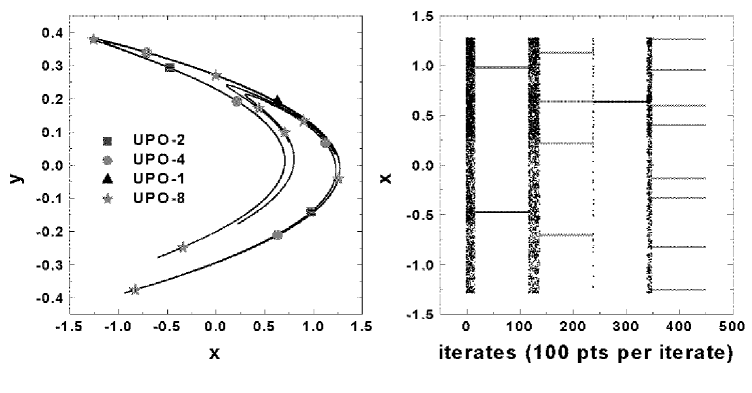
Figure 4: Hénon Map: The left panel shows the attractor with a number of embedded UPOs. The right panel shows the successive OGY control of UPOs of period 2, 4, 1, 8 for $a_{0}=1.4,$ $b_{0}=0.3$. The control is held for 10 000 iterates with $\delta=5\times 10^{-3}$ and $\delta a_{\rm max}=10^{-2}\ a_{0}$.

The Hénon map HEN76 has been a paradigmic example in nonlinear dynamics ever since its inception. It has the form
$\displaystyle x_{n+1}$ $\displaystyle=$ $\displaystyle 1-{a}\,x_{n}^{2}+y_{n}$ $\displaystyle y_{n+1}$ $\displaystyle=$ $\displaystyle b\,x_{n}$
and a Jacobian matrix given by

$${\mathbf{U}}=\left(\begin{array}[]{cc}-2ax&1\\ b&0\end{array}\right)$$ (38)

with determinant (the Jacobian) equal to $b$. It is dissipative for $|b|<1$ and possesses a non trivial strange attractor for various combinations of the parameters $a,|b|<1$. For our purpose, it serves as a benchmark, since the complete OGY strategy (eqns (18) or (22) or (24) ) can be performed (semi-) analytically and compared with other implementations. For example, the Jacobian matrices ${\mathbf{U}}_{i}^{(m)}$ are the product of $m$ individual Jacobian matrices along the periodic orbit, i.e. ${\mathbf{U}}_{i+m-1}\ {\mathbf{U}}_{i+m-2}\ \ldots\ {\mathbf{U}}_{i+1}\ {\mathbf{U}}_{i}$, whose eigenvectors can be written down analytically.

Our experiment (Fig. 4) shows the attractor for $a_{0}=1.4,b_{0}=0.3$ with the locations of embedded UPOs of periods 1, 2, 4, 8. The OGY control algorithm was used and the perturbations applied to the parameter $a_{0}$. The right panel of Figure (4) shows the values of the $x$ variable for a scenario involving the successive stabilizations of period 2, 4, 1, and 8. The target orbit is changed once a UPO has been controlled for 10 000 iterates. The control region was set to $\delta=5\times 10^{-3}$ and the maximum perturbation allowed was $\delta a_{\rm max}=10^{-2}\ a_{0}$. Under the same operational conditions, the MED minimization gave equally satisfactory results.

3D Rössler Flow

Figure 5: Rössler Attractor with an embedded UPO of period 3 in darker line. The flow parameters are $a_{0}=b_{0}=0.2$ and $c_{0}=5.7$ . Also indicated is the plane $x=2$ where dynamical informations are gathered.

Until now, our examples have described discrete dynamics and our formalism is also derived for maps. We now show how to appropriately discretize a flow to achieve control with the methods derived thus far. The Rössler system ROS79 consists of 3 coupled differential equations

$$\dot{x} = -y-z$$

$$\dot{y} = x+a\,y$$ (39)

$$\dot{z} = x\,z-{c}\,z+b$$

and a chaotic orbit is bounded to a funnel-like attractor (Fig. 5: $a_{0}=b_{0}=0.2,c_{0}=5.7$) where the motion is mostly in the $x-y$ plane with rapid excursions in the $z$ direction.

The last observation leads us to one possible discretization: one can register intersections of the flow with a plane $x={\rm cte}$ (the Poincaré section) and accumulate the pairs $(y_{n},z_{n})$ from which one could subsequently infer a map (the Poincaré map), $(y_{n+1},z_{n+1})={\mathbf{F}}_{P}((y_{n},z_{n}))$. For uniqueness, one must choose directed intersections by monitoring $\dot{x}$ on the Poincaré section (see Fig. 5).

The intersections with the Poincaré section ($x=2,\dot{x}>0$) is represented in the lower left panel of Figure (6). One notices little variation in the $z$ component and our quasi 1D control methods should be appropriate. In the same panel, one has indicated the positions of 3 UPOs to be stabilized. The OPF control of the $y$ component is shown in the lower right panel of Figure (6) resulting in 3 continuous trajectories (upper panel) embedded in the attractor (compare with Fig. 5). We believe that this success indicates just how robust this type of linear feedback is. Remember that we intervene in the dynamics only on the Poincaré section with a small perturbation (here $<1\%$ of $c_{0}$) at every $m$ intersections.

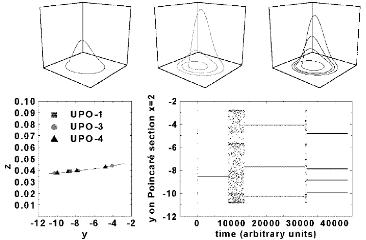
Figure 6: Rössler Flow: (upper panel) 3 stabilized continuous trajectories embedded in the attractor of Fig. 5; (lower left) locations of the UPOs on the Poincaré section $x=2,\dot{x}>0$; (lower right) OPF control on the Poincaré section of the $y$ components of the UPOs. Control is held during 1 500, 1 000, and 500 cycles for period 1, 3, and 4 respectively (1 cycle = 1 complete orbit) with $\delta=10^{-2}$ and $\delta c_{\rm max}=10^{-2}\ c_{0}$.

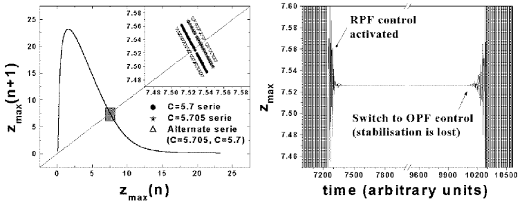
Figure 7: Rössler Flow: (left) first return map of successive maxima of the $z$ variable (Lorenz map) for the attractor of Fig. 5; (right) success of the RPF control and failure of the OPF method applied to the $z_{\rm max}$ series with $\delta=10^{-1}$ and $\delta c_{\rm max}=10^{-2}\ c_{0}$.

We have performed another experiment on the Rössler flow. It consists of collecting subsequent maxima $z_{n,{\rm max}}$ of the $z$ variable along a chaotic trajectory to construct a discretization of the flow. By plotting $z_{n+1,{\rm max}}$ versus $z_{n,{\rm max}}$, one obtains a (first) return map which is usually called a Lorenz map after the man who first defined the procedure. Our map is shown on the left of Figure (7) and it has all the characteristics of a chaotic 1D map. Again this indicates that our quasi 1D control (RPF or OPF) methods should be applicable. However, according to Figure (5), this should be rather delicate since the trajectory spends most of its time in the $x-y$ plane. In other words, the Lorenz map may not be adequate to gather enough dynamical information for control.

We have therefore used the RPF algorithm where $g_{u}$ and $g_{b}$ are first estimated by alternating the value of $c_{0}$ between 5.700 and 5.705. As expected, this creates two new applications $F_{u}$ and $F_{b}$ as clearly seen in the enlarged section of Figure (7). The right side of Figure (7) shows the RPF stabilization of a period 1 UPO which is maintained for 5 000 iterates before switching to the OPF algorithm where control is rapidly lost. The refinement incorporated in the RPF method has served us well and this experiment reveals nicely the limitation of the simplest strategy.

Billiard Dynamics

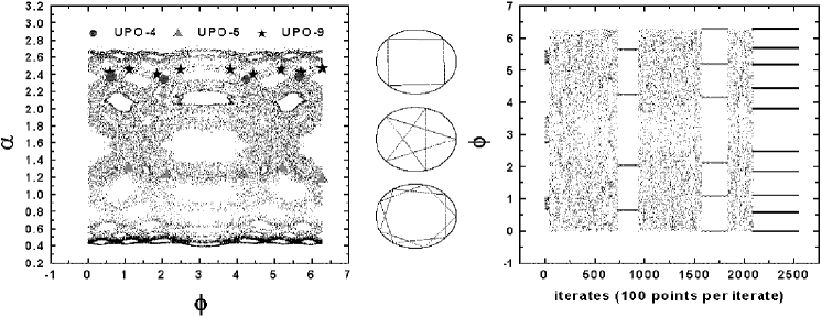
Figure 8: Cosine Billiard: (left) mixed chaotic (filled) and regular (open islands) phase space with embedded UPOs for $\epsilon_{0}=0.3$; (middle) MED controlled UPOs of period 4, 5 , 9; (right) stabilized $\phi$ variable of the corresponding UPOs held for 5 000 cycles each with $\delta=10^{-2}$ (1 cycle = 1 complete orbit).

The study of the frictionless motion of a particle bounded by a closed surface where it is specularly reflected is known as billiard dynamics and dates back to Birkhoff BIR27 . It serves to illustrate the transition from strict regularity (integrability) to chaos (ergodicity) in Hamiltonian systems billiard and bears important connections to quantum chaos as well billiard-qc . We have chosen to study the 2D cosine billiard where the surface is parametrized in polar coordinates by the relation

$$r(\phi)=1+{\epsilon}\,\cos\phi\quad.$$ (40)

The parameter $\epsilon$ is a measure of nonintegrability since for $\epsilon=0$, the curve is a circle and represents the integrable limit. For all $\epsilon\neq 0$, there are finite regions of phase space that contain chaotic trajectories. Figure (8) shows on the left the mixed and complex structure of phase space for $\epsilon_{0}=0.3$: the state variables are the incident angles on the surface, $\{\alpha_{n}\}$ , and the polar angles of the point of impact, $\{\phi_{n}\}$. Since motion is free in between collisions with the surface, our example belongs to the class of 2D area-preserving mappings, where attractors are absent and replaced by stochastic bands mixed with regular regions. Within these bands, the motion is ergodic: the blackened region is produced by one single chaotic orbit. Embedded in this stochastic web, one observes a number of UPOs whose physical trajectories inside the boundary are shown in the middle portion of Figure (8). By pulsating the deformation parameter $\epsilon$ about its nominal value, we have achieved control of 3 UPOs of period 4, 5 and 9. We used the MED control algorithm with a neighbourhood of $\delta=10^{-2}$. A numerical OGY method gives identical performance.

We mention that the successful control of billiard dynamics may offer a solution to the degradation of finesse in resonant optical microcavities NOC97 . It has been inferred that the loss of lasing activities might be associated with ray chaos (geometrical limit) in the optical resonators where the photons are transported (via chaotic diffusion) to regions of phase space where refractive escape (Snell’s law) becomes possible. The dielectric droplets making up the resonators behave very much like 2D billiards and we propose that programmed variations of the asymmetry may help reduce photon leakage. The viability of the proposal is currently being investigated.

Diamagnetic-Kepler Hamiltonian

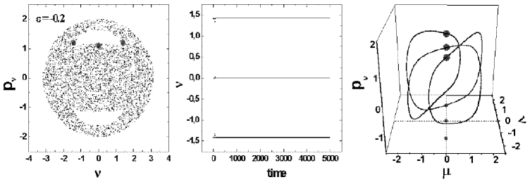
Figure 9: Diamagnetic Kepler Problem for scaled energy $\epsilon_{0}=-0.2$: (left) Poincaré section $\mu=0,\dot{\mu}>0$ showing one chaotic trajectory (filled space) and an OGY controlled period 3 orbit (black dots); (middle) the stabilized $\nu$ variable on the Poincaré section; (right) corresponding 3D trajectory. The control settings are $\delta=10^{-3}$ and $\delta\epsilon_{\rm max}=7\times 10^{-2}$.

Our final example is a continuous, 2 degrees of freedom (4D phase space) Hamiltonian system. It represents the motion of an electron under the combined influence of a Coulomb and a magnetic field. It goes under the name, diamagnetic Kepler problem (DKP), and occupies central stage in classical and quantum chaos research BLU97 . We use scaled semi-parabolic coordinates and write the resulting scaled (pseudo-) Hamiltonian as (for angular momentum $L=0$)

$$\hat{h}_{DK}=\frac{1}{2}(p^{2}_{\nu}+p^{2}_{\mu})-{\epsilon}\,(\nu^{2}+\mu^{2})+\frac{1}{8}\nu^{2}\mu^{2}(\nu^{2}+\mu^{2})\equiv 2\quad.$$ (41)

The scaled energy $\epsilon$ is related to the physical energy $E$ by $\epsilon=\gamma_{0}^{-2/3}\ E$ where the parameter $\gamma_{0}=B/B_{0}$ denotes the strength of the magnetic field relative to the unit $B_{0}\simeq 2.35\ 10^{5}\ T$. The classical flow covers a wide range of Hamiltonian dynamics reaching from bound, nearly integrable behaviour to completely chaotic and unbound motion as the scaled energy is varied dkp .

The dimension reduction (from 4D to 2D) and discretization is performed by observing the dynamics on the Poincaré section defined by $\mu=0,\dot{\mu}>0$. The energy shell is then mapped to an area bounded by the condition $p_{\nu}^{2}-2\epsilon\ \nu^{2}=4$ which represents an ellipse in the $(\nu,p_{\nu})$ plane. The left panel of Figure (9) shows the collection of points $\{\nu_{n},p_{\nu,n}\}$ obtained by numerical integration of the equations of motion for $\epsilon_{0}=-0.2$. One notices, for this energy, that phase space has few regular structures: apart from two lobes of regularity, the rest of the ellipse is filled by the successive piercings of one chaotic trajectory. The three dots indicate the positions of a UPO of period 3. We have succeeded in stabilizing a number of UPOs for the system, one of them is displayed with its 3D trajectory in Figure (9). We have employed a complete numerical implementation of the OGY strategy.

In attempting to bring order to the DKP dynamics, we had to overcome a number of difficulties not encountered in our previous examples. First, a typical trajectory spends a lot of time away from the Poincaré section and because of the sensitivity of the dynamics we had to device an efficient variable step symplectic integrator thereby preserving the geometrical structure of the Hamiltonian. Second, we had to obtain numerical Jacobians for all members of the UPOs since it was found to be necessary to intervene at every crossing of the Poincaré section. Third, the eigenvalues of area-preserving Jacobians are often complex and the stable and unstable manifolds are no longer along the directions of their eigenvectors. A new method had to be implemented. Details of the ingenious solutions to these problems can be found in POU99 .

We should comment that this is the first control of a realistic Hamiltonian system. It still remains an open question however if manipulations of the magnetic field to induce stabilization of a classical unstable orbit can be extended to the control, for example, of Rydberg wave packet dynamics.

Properties of the Control Procedure

The lessons learned through the previous examples and many more not reported here allow us to draw a list of the properties and advantages of the adopted control ‘philosophy’ and to point to remaining difficulties.
 
– no model dynamics is required a priori and only local information is needed;
– computations at each step are minimal;
– gentle touch: the required changes in $p_{0}$ can be quite small ($<1\%$ );
– multi-purpose flexibility: different periodic orbits can be stabilized for the same system in the same parameter range;
– control can be achieved even with imprecise measurements of eigenvalues and eigenvectors: the methods are robust;
– the methods can also be applied to synchronization of several chaotic systems.

At least three complications come to mind when one considers the implementation of chaos control strategies to the laboratory. The presence of noise, ignored so far, may induce occasional loss of control or hinder it altogether. The average waiting time to fall in the $\delta$-neighbourhood may be very (too) long, especially for Hamiltonian systems and a targeting strategy targeting should complement the control method. Furthermore, the system’s parameters may drift with time and this nonstationarity should be accounted for by updating the control informations. Tracking tracking is the name given to this procedure.

Conclusions and Future Perspectives

CHAOS often breeds life,
When ORDER breeds habit.

Henry Brooks ADAMS

We have presented the basic techniques for controlling chaos and we have reported on some of our efforts to recover order from chaos. Applications of the control of chaos have been reported in such diverse areas as aerodynamics, chemical engineering, communications, electronics, fluid mechanics, laser physics, as well as, biology, finance (not confirmed!), medicine, physiology, epidemiology and the list is constantly growing. It is perhaps instructive at this point to quote some of the earliest experimental successes of the methods to gain an idea of the breadth and diversity of the systems considered: in solid state devices and condensed matter, magneto-elastic ribbon DIT90 , spin-wave system AZE91 , electric diode HUN91 ; in fluid mechanics, regularization of chaotic convection SIN91 ; in chemistry, mechanisms of control of autocatalytic reactions PEN91 ; in laser systems, stabilization of coupled ensemble of lasers ROY92 ; in physiology, cardiac arrhythmia GAR92 , (anti)-control of epileptic seizures SCH94 .

The last decade has seen much accomplishments and challenges for the future are numerous. The following items seem to provide a glimpse of things to come: generalization to spatio-temporal chaos, adaptive control for non-stationary dynamics, effective control in the presence of noise (dynamical and/or observational), adaptive synchronization of chaos.

However, the greatest challenge will remain for some times the application to complex biological systems and in particular to brain dynamicsGOL92 . Despite early efforts, euphoria has been replaced by a healthy skepticism. Indeed, complex natural systems are noisy, contain a strong stochastic component and not endowed with a behaviour called chaos (at least not in its mathematical rigorous sense). Yet, one would like to believe that “the controlled chaos of the brain is more than an accidental by-product of the brain complexity” FRE91 . The perspective of unifying the techniques of deterministic chaos control with a statistical stochastic description as a possible therapeutic strategy against dynamical diseases is surely something to consider.

Acknowledgments. $\cal LJD$ thanks the members of his research group for their contributions and stimulating discussions on the subject. He is also grateful for the hospitality of G. Deco and B. Schürmann (München) where this work took its flight and to J. Honerkamp and J. Timmer (Freiburg) where this report was completed.

References

- (1) Dyson, F., Infinite in All Directions, New York: Harper and Row Publishers, 1988, chap. 10, pp. 182-184.
- (2) Poincaré, H., Acta Mathematica 13, 1 (1890).
- (3) Lorenz, E.N., J. of Atmos. Sci. 20, 130 (1963).
- (4) Ott, E., Grebogi, C., and Yorke, J.A., Phys. Rev. Lett. 64, 1196 (1990).
- (5) Ditto, W.L., Rauseo, S.N., and Spano, M.L., Phys. Rev. Lett. 65 , 3211 (1990).
- (6) Reyl, C., Flepp, L., Baddi, R., and Brun, E., Phys. Rev. E 47, 267 (1993).
- (7) Dressler, U., and Nitsche, G., Phys. Rev. Lett. 68, 1 (1992).
- (8) Rollins, R.W., Parmananda, P., and Sherard, P., Phys. Rev. E 47, R780 (1993).
- (9) Hunt, E.R., Phys. Rev. Lett. 67, 1953 (1991).
- (10) Ott, E., Sauer, T., and Yorke, J.A., eds., Coping with Chaos , New York: John Wiley & Sons Inc., 1994.
- (11) Eckman, J.P., Kamphorst, S.O., Ruelle, D., and Ciliberto, S., Phys. Rev. A 34 , 4972 (1986); Sanon, M., and Sawada, Y., Phys. Rev. Lett. 55 , 1082 (1985).
- (12) Takens, F., Lectures Notes in Math. 898 (1981); Sauer, T., Yorke, J.A., and Casdagli, M., J. Stat. Phys. 65, 579 (1991).
- (13) Shinbrot, T., Ott, E., Grebogi, C., and Yorke, J.A., Phys. Rev. Lett. 65 , 3215 (1990); Kostelich, E.J., Grebogi, C., Ott, E., and Yorke, J.A., Phys. Rev. E 47 , 305 (1993).
- (14) Hénon, M., Comm. Math. Phys. 50, 69 (1976).
- (15) Rössler, O.E., Phys. Lett. A 71 , 155 (1979).
- (16) Birkhoff, G.D., Acta Math. 50, 359 (1927).
- (17) Berry, M.V., Eur. J. Phys. 2, 91 (1981); Robnik, M., J. Phys. A 16 , 3971 (1983).
- (18) Stöckmann, H.J., and Stein, J., Phys. Rev. Lett. 64 , 2215 (1990); Stein, J., and Stöckmann, H.J., Phys. Rev. Lett. 68 , 2867 (1992).
- (19) Nöckel, J.U., and Stone D., Nature 385, 45 (1997).
- (20) Blümel, R., and Reinhardt, W.P., Chaos in Atomic Physics, Cambridge: Cambridge Uni. Press, 1997.
- (21) Delos, J.B., Knudson, S.K., and Noid, D.W., Phys. Rev. A 30 , 1209 (1984); Friedrich, H., and Wintgen, D., Phys. Rep. 183, 37 (1989).
- (22) Pourbohloul, B., Control and Tracking of Chaos in Hamiltonian Systems, Ph.D. Thesis (Université Laval, May 1999); Pourbohloul, B., and Dubé, L.J., Control and Tracking in the Diamagnetic Kepler Problem (submitted to Phys. Rev. Lett.)
- (23) Schwartz, I.B., Carr T.W., and Triandaff, I., Chaos 7 , 64 (1997).
- (24) Azevedo, A., and Rezende, S.M., Phys. Rev. Lett. 66 , 1342 (1991).
- (25) Singer, J., Wang, Y., and Bau, H., Phys. Rev. Lett. 66 , 1123 (1991).
- (26) Peng, B., Petrov, V., and Showalter, K., J. Phys. Chem. 95, 4957 (1991).
- (27) Roy, R., Murphy Jr., T.W., Maier T.D., Gills, Z., and Hunt, E.R., Phys. Rev. Lett. 68 , 1259 (1992).
- (28) Garfinkel, A., Spano, M.L., Ditto, W.L., and Weiss, J.N., Science 257, 1230 (1992).
- (29) Schiff, S.J., Jerger, K., Duong, D.H., Chang, T., Spano, M.L., and Ditto, W.L., Nature 370, 615 (1994).
- (30) Goldberger, A.L., in Applied Chaos, J. H. Kim and J. Stringer (Eds.), New York: John Wiley & Sons Inc., 1992, pp. 321-331.
- (31) Freeman, W.J., Scientific American Feb., 78 (1991).