Stability of the Ground State of a Harmonic Oscillator
in a Monochromatic Wave

Abstract

Classical and quantum dynamics of a harmonic oscillator in a monochromatic wave is studied in the exact resonance and near resonance cases. This model describes, in particular, a dynamics of a cold ion trapped in a linear ion trap and interacting with two lasers fields with close frequencies. Analytically and numerically a stability of the “classical ground state” (CGS) – the vicinity of the point ($x=0,p=0$) – is analyzed. In the quantum case, the method for studying a stability of the quantum ground state (QGS) is suggested, based on the quasienergy representation. The dynamics depends on four parameters: the detuning from the resonance, $\delta=\ell-\Omega/\omega$, where $\Omega$ and $\omega$ are, respectively, the wave and the oscillator’s frequencies; the positive integer (resonance) number, $\ell$; the dimensionless Planck constant, $h$, and the dimensionless wave amplitude, $\epsilon$. For $\delta=0$, the CGS and the QGS are unstable for resonance numbers $\ell=1,\,2$. For small $\epsilon$, the QGS becomes more stable with increasing $\delta$ and decreasing $h$. When $\epsilon$ increases, the influence of chaos on the stability of the QGS is analyzed for different parameters of the model, $\ell$, $\delta$ and $h$.

I Introduction

One of the major difficulties in developing quantum technologies, such as quantum computers, [1, 2] are different kinds of specifically quantum dynamical instabilities that can occur due to interactions between different degrees of freedom and resonant interaction with the external fields. Instabilities in quantum systems have different nature than instabilities in classical systems, in which such kind of phenomenon as dynamical chaos occurs as a result of exponential divergence of initially close trajectories. In quantum systems, the notion of a trajectory is not well defined. This is one of the main reasons why most of well-developed methods for stability analysis can not be directly applied to quantum systems.

In this paper the dynamics of a harmonic oscillator in a monochromatic wave field is studied. This system describes, in particular, a quantum dynamics of a cold ion trapped in a linear ion trap and interacting with two laser fields with close frequencies.[3] Our attention is focused mainly on classical and quantum behavior in the region of parameters close to the quantum ground state (QGS) of the harmonic oscillator. This case corresponds to classical dynamics in the vicinity of the point ($x=0,\,p=0$) in the phase space. We shall call the corresponding region of parameters for the classical system a “classical ground state” (CGS) of a harmonic oscillator. The stability of the CGS and the QGS at stable and chaotic classical regimes is analyzed for different parameters of the model. In Sec. II, we consider classical dynamics in the vicinity of the CGS in the exact resonance case, $\delta=0$. In this situation the system we study is degenerate,[4] and an infinitely small perturbation generates in the classical phase space an infinite number of the “resonance cells” separated by the infinite stochastic web. A classical dynamics inside the resonance cells at small $\epsilon$ is described by using the resonance perturbation theory.[5] It is shown, that in the vicinity of the CGS (the “central cell”), and for small enough $\epsilon$, the dynamics in the case $\delta=0$ is unstable for resonance numbers $\ell=1,2$ and stable for $\ell\geq 3$.

We show that in spite of the “resonant Hamiltonian” describes many features of the dynamics inside the resonance cells, it can not be used for describing the stability of the system in the central cell, at $\ell\geq 3$. The classical dynamics in this region is determined, by the Mathieu equation. It is shown that at small enough value of $\epsilon$ the area of the central cell increases with increasing the resonance number, $\ell$, and increasing the perturbation amplitude, $\epsilon$.

The dynamics of the system near the CGS in the near resonance case, when $\delta\neq 0$, is considered in Sec. III. It is shown that in this case at small $\epsilon$ the classical dynamics near the CGS is stable at any value of the resonance number $\ell$. The cases $\ell=1$ and $\ell=2$ are considered in detail. It is shown that the CGS in these two cases becomes unstable at much less values of $\epsilon$, than for large $\ell$ ($\ell=4,5$…).

A stability of the quantum system is considered in Sec. 4. In this case, an additional parameter, a dimensionless Planck constant, $h$, influences significantly the behavior of the system. Because the Hamiltonian is time-periodic, with the period $2\pi/\Omega$, we use the Floquet theory to study localization properties of quantum system in the region of the QGS. For $\epsilon\ll 1$, and small enough $h$, the quasienergy (QE) states can be conventionally divided into the following groups. The first group includes the QE states which belong to some particular “resonance cells” in the Hilbert space. These QE states are well-localized inside a given resonance cell. The second group includes the delocalized “separatrix” QE states which correspond to the classical stochastic web. Usually, these “separtrix” QE states are responsible for tunneling effects between different “resonance cells”, even for small $\epsilon$.[6]

We show that the QGS is stable when the following conditions are satisfied: (a) an existence of the QE state mainly localized in the QGS of the harmonic oscillator, (b) when $\epsilon\ll 1$ and chaos is weak, (c) small enough $h$, when one can neglect the tunneling phenomenon. When $h$ is larger than the size of the central cell, no QE state localized in the QGS of the harmonic oscillator was found. We show, that at small enough values of $\epsilon$, the stability of the QGS can be improved by choosing the non-resonant frequency of the wave, so that $\delta=\ell-\Omega/\omega\neq 0$.

For small enough $\epsilon$, a stability of the QGS is mainly determined by the structure of the QE state mostly localized at the QGS of the harmonic oscillator (QGS QE state). In the exact resonance case this particular QE state has a complicated structure. On the one hand, it is mostly localized on the QGS, but, on the other hand, it has the “separatrix” structure[7] and provides a tunneling from the region of the QGS to other resonance cells. In order to improve stability of the QGS, the separatrix structure should be destroyed by choosing $\delta\neq 0$.

In the exact and near resonance cases we study numerically the probability, $P_{0}$, for a particle to remain in the QGS, depending on $\epsilon$ and for different values of $h$, $\ell$ and $\delta$. When $\delta=0$ and $\epsilon$ is small, the dynamics depends on the value of the quantum parameter, $h$, which controls degree of delocalization of the QGS QE state. When $h$ is small, the probability of tunneling to other cells is small too, and $P_{0}$ decreases with $\epsilon$ increasing, because chaos makes the QGS QE state more delocalized. For large enough values of $h$, the dependence of $P_{0}$ on $\epsilon$ becomes more complicated because in this case we have two superimposing effects: the influence of chaos on the dynamics, and the effect of tunneling to the classically unacceptable cells. These two features make the dependence $P_{0}=P_{0}(\epsilon)$ non-monotonic. In the region of small $\epsilon$, $P_{0}$ increases with $\epsilon$ increasing. This behavior of $P_{0}$ can be explained as a result of destroying the delocalized QE states with increasing $\epsilon$. Further increase of $\epsilon$ leads to decreasing $P_{0}$. This behavior of $P_{0}$ is connected with delocalization of QE states due to increasing of the chaotic component. At large enough values of $\epsilon$, the dependence of $P_{0}$ on $\epsilon$ becomes more complicated, and generally must be considered using many QE states. It is shown that the value of $\delta$ influence significantly the stability of the QGS only at small $\epsilon\leq 1$. The stability of the QGS at $\ell=1,\,2$ and $\delta\neq 0$ is explored. It is shown that the QGS becomes unstable at much less values of the wave amplitude than in the case when $\ell$ is large. The derived in this paper results are important for understanding a stability of quantum dynamics in the vicinity of the ground state.

II Classical dynamics near the CGS in the case of exact resonance

The Hamiltonian of the harmonic oscillator in a monochromatic wave is,

$$H=\frac{p^{2}}{2M}+\frac{M\omega^{2}x^{2}}{2}+v_{0}\cos(kx-\Omega t)=H_{0}+V(x,t),$$ (1)

where $M$ is the mass of the particle, $p$ is the momentum, $k$ is the wave vector, $v_{0}$ is the amplitude of the perturbation, and $H_{0}$ is the Hamiltonian of the harmonic oscillator. In the first part of this section we discuss the case of the resonance, when $\Omega=\ell\omega$. It is known (see for example Ref. [4]) that under the resonance condition the infinitely small perturbation, $v_{0}$, is enough to generate in the classical phase space the infinite stochastic web. The web is inhomogeneous, and its width decays with decreasing the perturbation amplitude, $v_{0}$, and increasing $|p|$ and $|x|$. Inside the cells of the web a particle moves along stable closed trajectories.

To analyze the dynamics of the harmonic oscillator in a monochromatic wave, described by the Hamiltonian (1), it is convenient to use the resonance perturbation theory [5] discussed below. Let us perform a transformation from the variables ($p,x$) to the canonically conjugated variables ($\bar{J}_{\varphi},\,\varphi$),

$$x=(2\bar{J}_{\varphi}/M\omega)^{1/2}\sin\varphi=r(\bar{J}_{\varphi})\sin\varphi,$$ (2)

$$p_{x}=(2\bar{J}_{\varphi}M\omega)^{1/2}\cos\varphi=M\omega r(\bar{J}_{\varphi})\cos\varphi,$$ (3)

where $r(\bar{J}_{\varphi})=(2\bar{J}_{\varphi}/M\omega)^{1/2}$ is the amplitude of oscillations. It is more convenient to work with the dimensionless coordinate, $X=kx$, and the dimensionless momentum, $P=kp/M\omega$, which are related to the variables ($\bar{J}_{\varphi},\,\varphi$) by the formulas,

$$X=\rho(\bar{J}_{\varphi})\sin\varphi,$$ (4)

$$P=\rho(\bar{J}_{\varphi})\cos\varphi,$$ (5)

where $\rho(J_{\varphi})=\sqrt{X^{2}+P^{2}}=kr(J_{\varphi})$. In order to treat the time on the same ground as the phase $\varphi$ let us introduce the new pair of canonically conjugated variables, $(\bar{J}_{\beta},\,\beta)$, where $\beta=\Omega t$. The initial Hamiltonian (1) expressed through the new variables takes the form,

$$H=\bar{J}_{\varphi}\omega+\bar{J}_{\beta}\Omega+v_{0}\cos\left(\rho\sin\varphi-\beta\right).$$ (6)

It is independent of time, but describes the motion in the two-dimensional space. The nonlinear perturbation in Eq. (6) can be expressed in a series,

$$v_{0}\cos\left(\rho\sin\varphi-\beta\right)=v_{0}\sum_{m=-\infty}^{\infty}J_{m}(\rho)\cos\left(m\varphi-\beta\right),$$ (7)

where $J_{m}(\rho)$ is the Bessel function. Under the resonance condition, $\Omega=\ell\omega$, all terms in the sum (7) quickly oscillate and can be averaged out, except for one term with $m=\ell$. In this approximation, the Hamiltonian (6) is reduced to,

$$H=\bar{J}_{\varphi}\omega+\bar{J}_{\beta}\Omega+v_{0}J_{\ell}(\rho)\cos\left(\ell\varphi-\beta\right).$$ (8)

It is convenient to introduce new, resonance, variables, ($\tilde{I},\,\theta$), ($\tilde{J},\,\tilde{\beta}$), by using the generating function,

$$F=\tilde{I}\left(\ell\varphi-\beta\right)+\tilde{J}\beta,$$

The new Hamiltonian,

$$H=\tilde{I}(\ell\omega-\Omega)+\tilde{J}\omega+v_{0}J_{\ell}(\rho)\cos\theta,$$ (9)

where $\theta=\ell\varphi-\beta$, is independent of the variable $\tilde{\beta}$. Hence, $\tilde{J}=const$. The resonance Hamiltonian,

$$H_{\ell}(\rho,\theta)=H-\tilde{J}\omega=v_{0}J_{\ell}(\rho)\cos\theta,$$ (10)

(where we used the resonance condition $\ell\omega=\Omega$) is independent of time, unlike the initial Hamiltonian (1).

The Poincarè surfaces of section of the system described by the Hamiltonian (1) in variables ($X,\,P$) are shown in Figs. 1 (a) - 1 (e), for the cases $\ell=1,2,3,4,5$. The phase

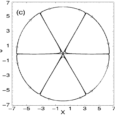
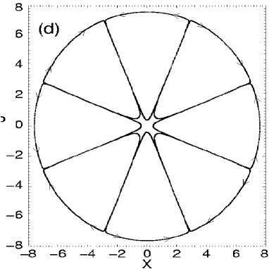
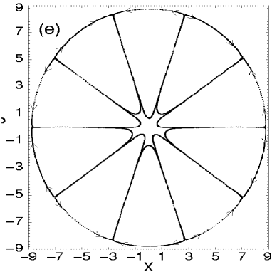
FIG. 1.: The resonance cells in the phase space for $\epsilon=0.05$, $\delta=0$ and: (a) $\ell=1$, (b) $\ell=2$, (c) $\ell=3$, (d) $\ell=4$, (e) $\ell=5$.

points are plotted at the moments $t_{j}=2\pi j/\Omega$, where $j=0,\,1,\,2,\dots$. One can see that the phase space has an axial symmetry of the order $\ell$. The phase space is divided into the cells. A particle moves along closed trajectories inside the cells. (In Figs. 1 (a) - 1 (e) only the boundaries of the cells are demonstrated.) At small values of $v_{0}$, the motion inside the resonant cells, illustrated in Figs. 1 (a) - 1 (e), can be considered in the resonance approximation. The next order approximation is required only for analysis of the motion inside the exponentially small chaotic regions near the separatrices. It is shown below that the resonance approximation also fails to describe the motion in the region near the point $(X=0,\,P=0)$.

The symmetry of the phase space in Figs. 1 (a) - 1 (e) follows from the form of the resonance Hamiltonian (10), which is invariant under the transformation,

$$\varphi\rightarrow\varphi+2\pi/\ell.$$ (11)

In the phase space there are $\ell$ cells connected by the transformation (11), and $\ell$ cells connected by the same transformation but described by the Hamiltonian $H_{\ell}(\rho,\theta+\pi)$ in Eq. (10). The total number of cells at given $\rho$ is $2\ell$. Thus, in Fig. 1 (a) the upper cell corresponds to the Hamiltonian $H_{1}(\rho,\theta)$, while the lower cell corresponds to the Hamiltonian $H_{1}(\rho,\theta+\pi)$ in Eq. (10); the upper and lower cells in Fig. 1 (b) correspond to $H_{2}(\rho,\theta)$, and the right and the left cells correspond to $H_{2}(\rho,\theta+\pi)$, and so on.

It is easy to see, the resonance Hamiltonian (10) yields unstable solution near the CGS (the point ($X=0,\,P=0$)). To show this, we present the Hamiltonian (10) in the form,

$$H_{\ell}=v_{0}\frac{\rho^{\ell}}{2^{\ell}\ell!}\cos\ell\varphi=E_{\ell},$$ (12)

where $E_{\ell}=const$ (because the resonance Hamiltonian is independent of time). Also, we took into account that at $\rho\ll 1$ the Bessel function can be expressed in the form,

$$J_{\ell}(\rho)\approx\rho^{\ell}/2^{\ell}\ell!,$$ (13)

and the fact that in the Poincarè surfaces of section the position of the particle is taken at the moments $\Omega t_{k}=2\pi k$, $k=0,\,1,\,2,\dots$. It follows from Eq. (12) that at the angles $\varphi_{k}=\frac{\pi}{2\ell}(2k-1)$, $k=1,\,2,\dots,\,2\ell$, the radius $\rho$ should sharply increase or decrease. It is seen from Figs. 1 (a) - 1 (e) that at angles $\varphi_{k}$ the particle moves in the radial direction. The grows of $\rho$ is limited due to nonlinear effects.

However, the resonance perturbation theory does not adequately describe the motion of a particle in the vicinity of the point ($X=0,\,P=0$) at large values of the resonance number $\ell$, because the amplitude of the resonance term due to Eq. (13) quickly decays when the radius, $\rho$, decreases. Indeed, at $\ell=4$ and $\rho=0.1$ the amplitude of the resonance term with $m=\ell=4$ in Eq. (7) is $80$ times less than the amplitude of the non-resonant term with $m=\ell-1=3$. In order to describe the motion in the region near the CGS, we consider the initial Hamiltonian (1) under the condition $X\ll 1$. The exact classical equation of motion reads,

$$\frac{d^{2}}{dt^{2}}X+\omega^{2}X=\frac{v_{0}k^{2}}{M}\sin(X-\Omega t).$$ (14)

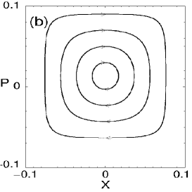
FIG. 2.: The trajectories in the central resonance cell in the phase space for $\delta=0$ and (a) $\ell=3$, $\epsilon=5\times 10^{-4}$, (b) $\ell=4$, $\epsilon=0.05$, (c) $\ell=5$, $\epsilon=0.05$.

Up to the first order in $X$ Eq. (14) is,

$$\frac{d^{2}}{dt^{2}}X+\omega^{2}(1-\epsilon\cos(\Omega t))X=\frac{v_{0}k^{2}}{M}\sin(\Omega t),$$ (15)

where $\epsilon=v_{0}k^{2}/M\omega^{2}$ is the dimensionless perturbation amplitude. If we introduce a new dimensionless time, $2\tau=\Omega t$, then from Eq. (15) we obtain the Mathieu equation with the additional right-hand side term in the form,

$$\frac{d^{2}}{d\tau^{2}}X+a_{\ell}(1-\epsilon\cos(2\tau))X=a_{\ell}\epsilon\sin(2\tau),$$ (16)

where $a_{\ell}=\left(2/\ell\right)^{2}$. From the theory of Mathieu functions [8] it is known that for small $\epsilon$, Eq. (16) has unstable general solutions at $a_{\ell}=1$ and $a_{\ell}=4$ which correspond to the resonance numbers, $\ell=2$ and $\ell=1$. The additional term in the right-hand side of Eq. (16) does not influence the stability of trajectories (see Ref. [8], §6.22). At $a_{\ell}<1$ and small enough values of $\epsilon$, the Mathieu equation has periodic solutions which correspond to the stable dynamics for resonance numbers $\ell>2$. In Fig. 2 stable trajectories in the system described by the Hamiltonian (1) are shown for $\ell=3,\,4,\,5$. Stable region in the vicinity of the CGS can be considered as additional “central cells” to those resonance cells shown in Figs. 1 (c) - 1 (e). The motion in the central cell is characterized by the following features: i) the size of the cell increases with increasing the resonance number, $\ell$; ii) trajectories in the cell have the axial symmetry of the order $\ell$; iii) as follows from numerical calculations, the period of the motion in the central cell along all trajectories in Figs. 2 (a) - 2 (c) is

FIG.3. The trajectories obtained by solution of Eq. (14) when only the terms up to (a) the first order (Eq. (16)) and (b) the fourth order in $X$ are taken into account; $\ell=5$, $\delta=0$, $\epsilon=0.05$.

approximately the same (in each figure), and very large. For example, the period of motion along the trajectories in Fig. 2 (b) for $\ell=4$ is $(1-1.2)\times 10^{5}T$, where $T=2\pi/\Omega$, while the period of motion along the trajectories in Fig. 1 (d) is of the order $\sim 5\times 10^{3}T$. The property i) can be described by the fact that the resonance term, which leads to unstable solution near the point ($X=0,\,P=0$), for larger values of $\ell$ has less influence on the dynamics because its amplitude at $\rho\ll 1$ quickly decreases with $\ell$ increasing, due to Eq. (13).

In order to treat the properties ii), iii), we have considered the influence of the terms of higher order in $X$ in Eq. (14) on the dynamics described by Mathieu equation (16). The results for the case $\ell=5$ are shown in Figs. 3 (a), 3 (b). From Figs. 3 (a), 3 (b) it is seen that the terms of high order in $X$ change the shape of trajectories, and make them symmetrical with the axial symmetry of the order $\ell$. This fact follows also from comparison of different trajectories in Fig. 2 (c). Indeed, internal trajectories with small values of $\rho$ have the round form, unlike external trajectories with larger values of $\rho$, which have the form of the pentagon. From comparison of Figs. 2 (c) and 3 (b) it is clear that the terms of high order in $X$ (the terms of the order $X^{i}$ where $i>\ell-1$) in Eq.(14) do not influence significantly the dynamics, because the form of trajectories in Fig. 3 (b), computed for the approximate model, is practically the same as the form of trajectories in the exact model shown in Fig. 2 (c).

It was established numerically that slowness of the motion in the vicinity of the CGS is also result of influence of the terms of high order in $X$. Thus, the period of motion along the external trajectory described by the approximate equation (16) in Fig. 3 (a) is $\sim 4\times 10^{4}T$. Including into consideration the second order term in $X$ increases the period of motion up to $\sim 3.3\times 10^{5}T$. If we include, as well, the third order term, the period becomes $\sim 3.6\times 10^{5}T$. Finally, including the resonance term leads to increase of the period up to the value $\sim 3.8\times 10^{5}T$ shown in Figs. 2 (c) and 3 (b).

Next, we shall analyze the dynamics in the central cell depending on $\epsilon$. Modification of trajectories at increasing the wave amplitude, $\epsilon$, for the resonance number $\ell=4$ is shown in Figs. 4 (a) - 4 (d). Two features in the structure of the trajectories of the central cell can be observed. i) Increase in $\epsilon$ shifts the central cell up. ii) The size of the cell increases considerably in Figs. 4 (a) - 4 (c) with increasing $\epsilon$ in comparison with the case shown in Fig. 2 (b), when the value of $\epsilon$ is very small. The cell shrinks when $\epsilon$ increases, which is shown in Fig. 4 (d) for $\epsilon=10$. Further increase of $\epsilon$ destroys the central cell entirely.

FIG. 4.: Trajectories in the central resonance cell at $\ell=4$, $\delta=0$ under influence of the perturbation with the amplitude, $\epsilon$: a) $\epsilon=0.5$, b) $\epsilon=2$, c) $\epsilon=5$, d) $\epsilon=10$.

Similar features were observed in dependence of the dynamics in the central cell on $\epsilon$ for the case $\ell=5$, shown in Figs. 5 (a) - 5 (d). Comparison of the data for $\ell=5$ in Figs. 5 (a) - 5 (d) with those for $\ell=4$ in Figs. 4 (a) - 4 (d) allows us to conclude that the area of the central cell increases with increasing $\ell$, and chaotization of the motion in the central cell at

FIG. 5.: Trajectories in the central resonance cell at $\ell=5$, $\delta=0$ under influence of the perturbation with the amplitude, $\epsilon$: a) $\epsilon=5$, b) $\epsilon=10$, c) $\epsilon=15$, d) $\epsilon=19$.

larger values of $\ell$ requires larger values of $\epsilon$. In other words, the motion in the central cell becomes more stable with increasing the resonance number, $\ell$. In order to understand the observed dynamics, we again included into consideration only the first order terms in $X$ in Eq. (14), and computed the dynamics for large values of $\epsilon$. The trajectories described by the approximate equation (16) for $\epsilon=5$, $\ell=4$ and for $\epsilon=9.5$, $\ell=5$ are shown in Figs. 6 (a), 6 (b). The following features can be observed. i) As follows from our calculations,

FIG. 6. The phase trajectories described by the approximate equation (16) for $\delta=0$ and (a) $\ell=4$, $\epsilon=5$, (b) $\ell=5$, $\epsilon=9.5$.

the phase portrait shifts up from the point $(X=0,\,P=0)$ under the influence of the term in the right-hand side of the approximate equation (16). ii) Comparison of Fig. 6 (a) with Fig. 4 (c) and Fig. 6 (b) with Fig. 5 (b) allows us to conclude that the terms of the high order in $X$ in Eq. (14) change the shape of trajectories and restrict the region of stable motion. iii) The motion described by the approximate equation (16) becomes unstable at values of $\epsilon>\epsilon_{\ell}$ where $\epsilon_{\ell}$ lies in the interval $2.3<\epsilon_{3}<2.4$ for $\ell=3$; $5.5<\epsilon_{4}<5.6$ for $\ell=4$; and $9.6<\epsilon_{5}<9.7$ for $\ell=5$. One can see from Fig. 4 (d) and Figs. 5 (c), 5 (d) that the motion described by exact equation (14) in the region $\epsilon>\epsilon_{\ell}$ remains stable. Thus, the high order terms in $X$ in Eq. (14) stabilize the dynamics at large values of the perturbation amplitude, $\epsilon$.

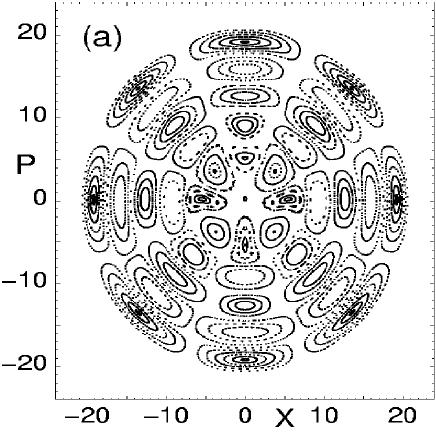
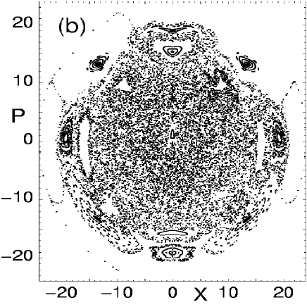
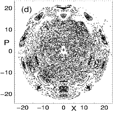
FIG. 7.: Influence of chaos on different resonant cells, $\delta=0$, (a) $\ell=4$, $\epsilon=1$; (b) $\ell=4$, $\epsilon=5$; (c) $\ell=5$, $\epsilon=1$; (d) $\ell=5$, $\epsilon=5$.

Let us compare the classical dynamics in the central cell with the dynamics in the other cells when the perturbation parameter $\epsilon$ is not small. The results of calculation of the dynamics in several cells are shown in Figs. 7 (a) - 7 (d). From comparison Fig. 7 (b) with Figs. 4 (c), 4 (d) and Fig. 7 (d) with Figs. 5 (a) - 5 (d) one can see that the trajectories in the central cell remain stable, while other nearest cells are completely destroyed by chaos. The extremely high stability of trajectories in the central cell can be explained by relatively small influence on the dynamics of the terms of high order in $X$, oscillating with different frequencies, because their amplitudes are small at small $X$ (or $\rho$).

III The classical dynamics near the CGS in the near resonance case

Now, let us consider the CGS in the near resonance case, when $\delta\neq 0$. The resonant Hamiltonian (9) takes form

$$H_{\ell}=\tilde{I}(\delta\omega)+v_{0}J_{\ell}(\rho)\cos\theta.$$ (17)

The stationary points for the dynamics generated by the Hamiltonian (17) are defined by the conditions,

$$\dot{\theta}=\partial H_{\ell}/\partial\tilde{I}=0,\qquad\dot{\tilde{I}}=-\partial H_{\ell}/\partial\theta=0.$$

Positions of the elliptic stationary points are given by the expressions,

$$v_{0}{\partial J_{\ell}[kr(\tilde{I}_{e})]\over\partial\tilde{I}}=\mp\delta\omega,\qquad\theta_{e}=0,\pi,$$ (18)

where the sing $``-^{\prime\prime}$ corresponds to the stable point, with the angle $\theta_{e}=0$ with the $P$-axis, and the sing $``+^{\prime\prime}$ corresponds to the stable point with the angle $\theta_{e}=\pi$. In the dimensionless form Eq. (18) is,

$$\frac{1}{\rho_{e}}{\partial J_{\ell}(\rho_{e})\over\partial\rho}=\mp{\delta\over\ell\epsilon},$$ (19)

where $\rho_{e}=kr(\tilde{I}_{e})$. For the positions of the hyperbolic stationary points one has,

$$J_{\ell}\left[kr(\tilde{I}_{h})\right]=0,\qquad\theta_{h}=\pm\frac{\pi}{2}.$$ (20)

As one can see from Eq. (19), the number of the elliptic stable points in the near resonance case, when $\delta\neq 0$, is finite because the right-hand side of Eq. (19) is constant while the left-hand side oscillates, and decreases on average. As a consequence, there is a finite number of the resonance cells.

The motion near the CGS can be described by the approximate equation (16) with the parameter $a_{\ell}$ equal to: $a_{\ell}=[2/(\ell-\delta)]^{2}$. It is known [8] that at small $\epsilon$ and $\delta\neq 0$ the Mathieu equations have the stable solutions at any $\ell$ including the cases $\ell=1$ and $\ell=2$.

Let us consider the cases $\ell=1$ and $\ell=2$ at $\delta\neq 0$ in detail. In the case $\ell=1$, one may use the results of the resonance theory at arbitrary small $X$ and $P$, because the term of the lowest order in $X$ (proportional to $X$) in the Hamiltonian (1) is resonant. Let us suppose that the dimensionless radius $\rho_{e}$ in Eq. (19) is small, $\rho_{e}\ll 1$. Then $J_{1}^{\prime}(\rho_{e})\approx 1/2$, and Eq. (19) yields,

$$\rho_{e}=\mp\epsilon/(2\delta\ell).$$ (21)

Thus, shift of the stable elliptic point from the CGS is small, $\rho_{e}\ll 1$, when the condition $\epsilon\ll 2|\delta|\ell$ is satisfied. At small values of the wave amplitude, $\epsilon$, shift of the elliptic stable point from the point $X=0,\,P=0$ is proportional to $\epsilon$. One can see from Eq. (21) that at $\ell=1$ one elliptic stable point exists at arbitrary small value of $\epsilon$ (which follows also from the theory of Mathieu functions).

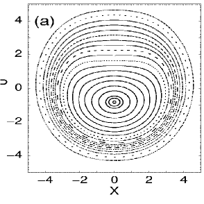
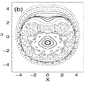
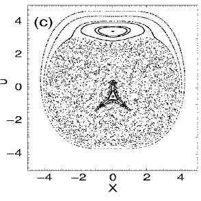
FIG. 8.: The phase space for the near resonance case, $\delta=0.1$, $\ell=1$, and (a) $\epsilon=0.4$, (b) $\epsilon=0.7$, (c) $\epsilon=1.2$

When $\epsilon$ is small, the phase trajectories are the circles with the center located near the CGS. Figuratively speaking, in the case $\delta\neq 0$ and $\epsilon\ll 1$ there is only one resonant (central) cell with an infinite area, because at small enough value of $\epsilon$ the equation (19) has no other solutions, except for Eq. (21), and in the phase space there are no other cells, except for the central one. When $\epsilon$ increases (we suppose $\epsilon>0$) and $\delta>0$, the stable point shifts down, as shown in Fig. 8 (a), because the left-hand side of Eq. (19) is positive and we should take the sign “$+$” in the right-hand side, which corresponds to the shift in the direction $\theta=\pi$.

When $\epsilon$ increases (see Fig. 8 (b), 8 (c)), the dynamical chaos appears, and the area of the central cell decreases. As before, we have considered the influence of the high order terms in $X$ in the exact equation of motion (14) on the dynamics described by the approximate equation (16). The approximate equation (16) yields unstable solutions when $\epsilon>\epsilon_{1}$, where $|\epsilon_{1}|=\sqrt{24|\delta|/5}$ if $\delta>0$, and $\epsilon_{1}=\sqrt{24|\delta|}$ if $\delta<0$.[9] The parameter $\delta=0.1$ yields $\epsilon_{1}=0.69$. As one can see from Figs. 8 (b), 8 (c) the central cell remains undestroyed. Thus, the nonlinear terms stabilize the dynamics in the near resonance case, similar to the case of exact resonance. At $\epsilon=1.2$ in Fig. 8 (c) one more cell is generated, because the condition (19) is satisfied for two values of $kr$.

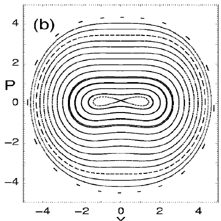
FIG. 9.: The phase space for the near resonance case, $\delta=0.1$, $\ell=2$, and (a) $\epsilon=0.17$, (b) $\epsilon=0.22$

Unlike the case $\ell=1$, when $\ell=2$ and $\epsilon$ is small enough (see Figs. 9 (a)), the stable point does not shift from the point $(X=0,\,P=0)$. Instead, in Fig. 9 (b) we observe bifurcation at the value $\epsilon=\epsilon_{2}$, where $\epsilon_{2}$ can be estimated from the solution of the approximate equation (16). Namely, up to the second order in $\delta$, the dynamics becomes unstable at $\epsilon_{2}=2\delta-\delta^{2}/2$.[9] Our computed value of $\epsilon_{2}$ lies in the interval $0.185<\epsilon_{2}<0.186$ which is slightly less than the estimated quantity due to the influence of nonlinear in $X$ terms, which are neglected in the approximate equation (16).

FIG. 10.: The same as in Figs. 9 (a), 9 (b) but for $\epsilon=0.8$

As shown in Fig. 10, at further increase of $\epsilon$, two stable points, formed after bifurcation, diverge at larger distance from each other, the chaotic area increases, and additional cells appear because the condition (19) is satisfied for more number of points ($kr(\tilde{I}_{e})$).

IV Stability of the quantum ground state

Now we consider a stability of the ground state of the quantum harmonic oscillator (QGS) under the same conditions as in the classical model. The quantum Hamiltonian is,

$$\hat{H}=\frac{\hat{p}^{2}}{2M}+\frac{M\omega^{2}}{2}x^{2}+v_{0}\cos(kx-\Omega t)=\hat{H}_{0}+\hat{V}(x,t),$$ (22)

where $\hat{p}=-i\hbar\partial/\partial x$, and the same notation as in Eq. (1) where used. Since the Hamiltonian (22) is periodic in time, we can use the Floquet theorem, and write the solution of the Schrödinger equation in the form,

$$\psi_{q}(x,t)=\exp(-iE_{q}t/\hbar)u_{q}(x,t),$$ (23)

where $E_{q}$ is the quasienergy, $\psi_{q}(x,t)$ is the quasienergy (QE) eigenfunction, and the function $u_{q}(x,t)$ is periodic in time, $u_{q}(x,t)=u_{q}(x,t+T)$, where $T=2\pi/\Omega$. We expand $u_{q}(x,t)$ in the basis of the unperturbed harmonic oscillator,

$$u_{q}(x,t)=\sum_{n=0}^{\infty}C_{n}^{q}(t)\psi_{n}(x),$$ (24)

where coefficients, $C_{n}^{q}(t)$, are periodic in time, $C_{n}^{q}(t)=C_{n}^{q}(t+T)$. Due to periodicity of $C_{n}^{q}(t)$, the approach based on Floquet states is very convenient for investigation of localization properties of the quantum system. Namely, if some initial state coincides with the quasienergy function localized in some region of the Hilbert space, $C_{n}(0)=C_{n}^{q}(0)$, then it will remain localized in this region for any time.

We used the following numerical procedure to calculate the QE states. [10, 11, 12] The QE states are the eigenstates of the evolution operator for one period of the wave field, $\hat{U}(T)$. In order to build the matrix $U_{nm}$ of the operator $\hat{U}(T)$ we choose the representation of the Hamiltonian $\hat{H}_{0}$. Let us act with the evolution operator on the wave function $\psi(x,0)$,

$$\hat{U}(T)\psi(x,0)=\psi(x,T),$$ (25)

and choose the initial state in the form $C_{n}(0)=\delta_{n,n_{0}}$. In this way we obtain a column in the evolution operator matrix,

     

     

FIG. 11.: The plots of averages versus dispersions for $h=0.5$, $\delta=0$ and (a) $\ell=1$, $\epsilon=0.05$, (b) $\ell=2$, $\epsilon=0.05$, (c) $\ell=3$, $\epsilon=5\times 10^{-4}$, (d) $\ell=4$, $\epsilon=0.05$, (e) $\ell=5$, $\epsilon=0.05$.

$$U_{n,n_{0}}=C_{n}^{(n_{0})}(T),$$ (26)

where the coefficients, $C_{n}^{(n_{0})}(T)$, can be obtained by numerical solution of the Schrödinger equation (for more detailed discussion see Ref. [7]). After diagonalization of $U_{n,m}$, we obtain the QE functions, $C_{n}^{q}\equiv C_{n}^{q}(mT)$, $m=0,\,1,\,2,\dots$ and the quasienergies, $E_{q}$. The values of matrix elements, $U_{n,m}$, depend on three dimensionless parameters: the wave amplitude, $\epsilon$, the quantum parameter, $h=k^{2}\hbar/M\omega$, which can be treated as a dimensionless Planck constant, and from the ratio $\Omega/\omega=\ell-\delta$.

   

FIG. 12.: The probability distribution for the QGS QE states with the smallest average, $n_{q}$, for the cases (a) $\ell=4$, (b) $\ell=5$; $\epsilon=0.05$, $h=0.5$, $\delta=0$.

When $\delta=0$ and the amplitude of the wave is small, $\epsilon\ll 1$, most of the QE states are divided into almost independent groups, each located in one resonance cell of the Hilbert space. [6] In order to show this let us characterize each QE state by its average, $n_{q}=\sum_{n}n|C_{n}^{q}|^{2}$, and a dispersion, $\sigma_{q}=\left[\sum_{n}(n-n_{q})^{2}|C_{n}^{q}|^{2}\right]^{1/2}$ and plot $n_{q}$ versus $\sigma_{q}$ (see also Ref.[13]). Such plots for different values of the resonance number, $\ell$, and for small value of the wave amplitude, $\epsilon$, are shown in Figs. 11 (a) - 11 (e). The boundaries of the cells are marked by arrows. The radius of the external boundary of classical cells in Figs. 1 (a) - 1 (e) corresponds to the position of the boundary of the first quantum cell, respectively, in Figs. 11 (a) - 11 (e) with the quantized radius, $\rho_{n}=\sqrt{2nh}$. One can see from Figs. 11 (a) - 11 (e) that the QE states are mostly located within the quantum resonance cells, because their averages, $n_{q}$, are situated inside the cells, and their widths, $\sigma_{q}$, do not exceed the width of the corresponding resonance cell. Such states form rows in Figs. 11 (a) - 11 (e). Each cell in the Hilbert space in the quasiclassical limit corresponds to $2\ell$ classical cells. [14] There also exist the QE states which do not belong to a particular resonance cell, but rather they belong to the stochastic web. These QE states have a “separatrix” structure, i.e. they delocalized over several resonance cells and have large dispersion, $\sigma$. Such states are represented by scattered points on the diagrams $n_{q}=n_{q}(\sigma_{q})$ in Figs. 11 (a) - 11 (e). The structure of these QE states was in details discussed in Refs. [6, 7, 15].

     

FIG. 13.: The same as in Figs. 12 (a), 12 (b) but in the logarithmic scale.

In this paper, we focus on the QE states which belong to the central resonance cell (QGS QE states), because these states are mainly responsible for stability properties of the QGS. Such QGS QE states are characterized by small average, $n_{q}$, and are located in the low part of the plots, $n_{q}(\sigma_{q})$, in Figs. 11 (d), 11 (e). In the cases $\ell=1,2$ in Figs. 11 (a) - 11 (b) these states are absent, which corresponds to unstable dynamics near the CGS in the phase classical space, shown, respectively, in Figs. 1 (a) - 1 (b). In the case $\ell=3$, the area of the stable island in Fig. 2 (a) is much less than the value of the dimensionless Planck constant $h$ ($h=0.5$). So, in this case, the QGS QE state is absent, too.

The plots of the probability distribution for the QGS QE states $q^{\prime}$ with the smallest average, $n_{q^{\prime}}$, marked in Figs. 11 (d), 11 (e) by arrows, are shown in Figs. 12 (a), 12 (b), for the cases $\ell=4$ and $\ell=5$. In the logarithmic scale, these states are illustrated in Figs. 13 (a), 13 (b). The Husimi functions of these states are shown in Figs. 14 (a) ($\ell=4$) and 14 (b) ($\ell=5$). As one can see from Figs. 12 (a), 12 (b) the QGS QE state is mainly localized in the CGS of the harmonic oscillator. One can see from Figs. 12 (a), 12 (b) and 13 (a), 13 (b) that the small part of the probability distribution is located at the levels with the numbers $n=\ell m$, where $m=1,\,2,\dots$. This can be explained by influence of the resonance terms in the quantum equations of motion.[6] In the resonance approximation the QE states can be defined from the set of algebraic equations which in the dimensionless form can be written as,

$$\left({E_{q}\over\hbar\omega}-\delta n\right)C_{n}^{q}=\frac{\epsilon}{h}(V_{n,n+\ell}C_{n+\ell}^{q}+V_{n,n-\ell}C_{n-\ell}^{q}).$$ (27)

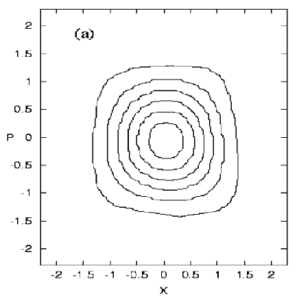
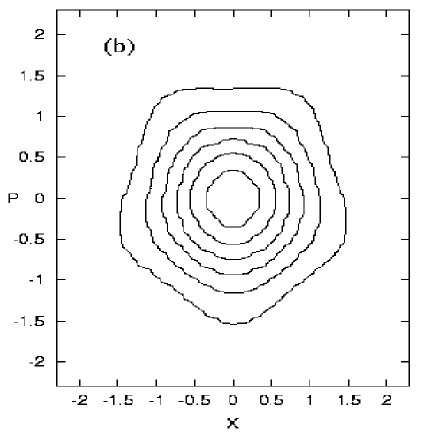
FIG. 14.: (a) The Husimi functions of the QGS QE state shown in Fig. 12 (a). (b) The Husimi functions of the QGS QE state shown in Fig. 12 (b). The cross-sections are plotted from the level $0.047$ with the increment $0.042$, $h=0.5$, $\epsilon=0.05$.

The matrix elements for $n\gg 1$ can be approximated by the Bessel functions $J_{m}$,

$$V_{n,n+2m+1}=\frac{1}{2}\frac{(-1)^{m}n^{m+1/2}e^{-\frac{h}{4}}}{\sqrt{(n+1)\dots(n+2m+1)}}J_{2m+1}(\sqrt{2nh}),$$ (29)

$$V_{n,n+2m}=\frac{1}{2}\frac{(-1)^{m}n^{m}e^{-\frac{h}{4}}}{\sqrt{(n+1)\dots(n+2m)}}J_{2m}(\sqrt{2nh}).$$ (30)

As one can see from Eq. (27), in the resonance approximation the QE functions have the form $C_{n}^{q}=C_{\ell m}^{q}$ with $m=1,\,2,\dots$. In this case, the particle is allowed to move only between the states with the numbers $n=\ell m$. As shown in Ref. [14], a particular form of the QE function, $C_{n}^{q}=C_{\ell m}^{q}$, makes the Husimi functions, illustrated in Figs. 14 (a) and 14 (b), symmetric with the axial symmetry of the order $\ell$. One can see that the width of the Husimi distribution in Figs. 14 (a) and 14 (b), is, $\Delta P\sim\Delta X\sim\sqrt{h}\sim 0.7$.

  

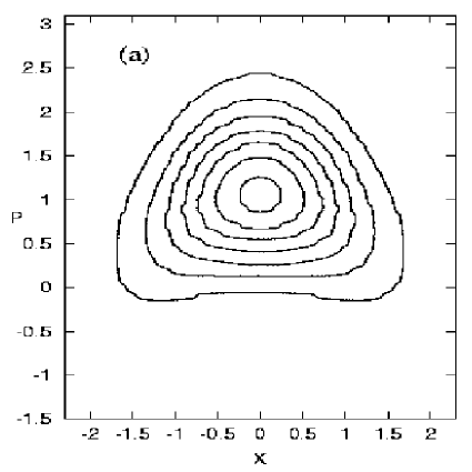
FIG. 15.: (a) The Husimi functions of the shifted from the ground state QE function, shown in Fig. 15 (b). The cross-sections are plotted from the level $0.047$ with the increment $0.042$, $\epsilon=5.0$, $h=0.5$.

Now, let us consider influence of dynamical chaos on the QE states, when $\epsilon$ increases. There are several QE states localized near the QGS of the harmonic oscillator. Some of them are shifted from the level with the number $n=0$. They can be associated with shifted up classical central resonance cell, when $\epsilon$ increases. In this case, the Husimi function in Fig. 15 (a) of the QE state with the probability distribution illustrated in Fig. 15 (b) (for $\ell=5$ and $\epsilon=5$) has a similar form to the form of the trajectories in the classical phase space shown in Fig. 5 (a). At large enough values of the wave amplitude, ($\epsilon=5$ in Fig. 15 (a)), there are no QE states localized in the nearest quantum cells, except for the QE states localized in the central cell. This corresponds to the chaotic classical dynamics shown in Figs. 7 (b), 7 (d) with the stable island in the center of the phase space.

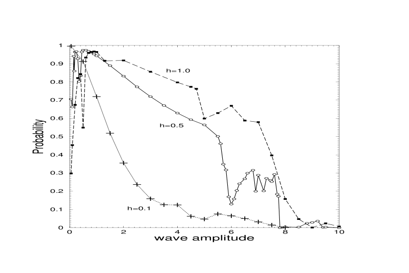
FIG. 16.: The probability to find the system in the QGS of the harmonic oscillator, defined by the values $|C_{n=0}^{q^{\prime}}|^{4}$ of the QE state $q^{\prime}$ mostly localized at the state with $n=0$, versus the wave amplitude, $\epsilon$, for three values of the effective Planck constant, $h$; $\ell=5$.

The QGS QE states, mostly localized at the CGS of the harmonic oscillator, are of the most interest for us, because they mainly define the dynamics of the quantum state initially located at the level with $n=0$. The time-evolution of the system with the initial state $C_{n}(0)=\delta_{n,n_{0}}$ is defined by the equation,

$$C_{n}(mT)=\sum_{q}C_{n}^{q*}C_{n_{0}}^{q}\exp(-iE_{q}mT/\hbar),$$ (31)

where $m=0,\,1,\,2,\dots$. The amplitude of probability to find the system in the initial state, $n_{0}$, is,

$$C_{n_{0}}(mT)=\sum_{q}|C_{n_{0}}^{q}|^{2}\exp(-iE_{q}mT/\hbar).$$ (32)

Suppose that some QE state with the number $q^{\prime}$ is mostly localized at the level $n=n_{0}$, i.e. $|C_{n_{0}}^{q^{\prime}}|^{2}\gg|C_{n_{0}}^{q}|^{2}$ for all $q\neq q^{\prime}$. Then, the term with $q=q^{\prime}$ dominates in the sum in the right-hand side of Eq. (32), and we can write,

$$C_{n_{0}}(mT)\approx|C_{n_{0}}^{q^{\prime}}|^{2}\exp(-iE_{q^{\prime}}mT/\hbar).$$ (33)

The probability, $P_{n_{0}}(mT)$, to find the system at the moments $t_{m}=mT$ in the state with $n=n_{0}$ is given by,

$$P_{n_{0}}(mT)=|C_{n_{0}}(mT)|^{2}\approx|C_{n_{0}}^{q^{\prime}}|^{4}.$$ (34)

The value of $P_{n_{0}}(mT)$ in this approximation is independent of the number of periods passed, $P_{n_{0}}(mT)\equiv P_{n_{0}}$. In the next approximation, the neglected terms in Eq. (32) cause the probability $P_{n_{0}}$ slightly oscillate with time.

In Fig. 16, we present a plot of the probability, $P_{0}=|C_{n_{0}=0}^{q}|^{4}$, to find the system in the QGS as a function of the wave amplitude, $\epsilon$, if the initial state is the QGS of the harmonic oscillator. One can see that the dynamical chaos (the range of large enough $\epsilon$) decreases this probability. However, the process of delocalization of the QGS QE state is extremely slow when $\epsilon$ increases, in comparison with that in other nearest cells. For example, at $\epsilon=5$ all QE states in the nearest cells are chaotic (delocalized) which corresponds to the chaotic classical dynamics in Fig. 7 (d), while the QE state located at the QGS remains localized with the probability $P_{0}\approx 0.56$ when $h=0.5$, and $P_{0}\approx 0.6$ when $h=1.0$. From comparison

                 

FIG. 17.: (a) The QE states mostly localized at the QGS of the harmonic oscillator (QGS QE states), $h=0.5$, (a) $\epsilon=0.05$, (b) $\epsilon=0.5$, (c) $\epsilon=5.5$ (d) $\epsilon=6.0$, (e) $\epsilon=7.6$, (f) $\epsilon=9.2$. The boundaries of the quantum cell are marked by arrows.

of different curves, for h=0.1, $h=0.5$ and $h=1.0$, one can note the following features. i) At small values of $\epsilon$, increase of $h$ leads, on average, to decrease of stability of the QGS. ii) The QGS, at large values of $h$ ($h=1$), is more stable under the influence of chaos (the range of large enough $\epsilon$) than that at small values of $h$ ($h=0.1$). We should note, that oscillations of $P_{0}(mT)$ in time should increase when $P_{0}(mT)$ decreases. This happens in the region of large enough $\epsilon$ in Fig. 16, because in this case the influence of neglected terms in Eq. (32) becomes more significant.

More information about the stability of the QGS can be extracted from the analysis of the structure of QE states located at the QGS at different values of the wave amplitude, $\epsilon$, shown in Fig. 17 (a) - 17 (f) (for $h=0.5$). The QGS QE state shown in Fig. 17 (a) for small value of $\epsilon$ ($\epsilon=0.05$) is similar to the separatrix QE states, [7] because it has the regular structure (compare, for example, with Fig. 17 (c)), and its maxima are located near the quantum separatrices, indicated in Fig. 17 (a) by arrows. Thus, the QGS QE state also possesses the properties of the “separatrix” QE states, considered in Ref. [7].

The separatrix QE states are of the quantum nature [7] because they are delocalized over several resonance cells. These QE states provide the tunneling between the cells when chaotic regions in the phase space are negligible small, and the classical particle can not practically penetrate from one resonance cell to another. The separatrix QE function mostly localized in the QGS is a particular one, and it is different from other separatrix states studied before.[7] On the one hand, it is delocalized over several resonance cells (see Fig. 17 (a)) as other separatrix QE functions. On the other hand, this particular QE function is mostly concentrated on the QGS of the harmonic oscillator, unlike the other separatrix QE functions. These “contradictory” features of the QGS QE state define the dynamics: on the one hand, the system mainly remains localized in the QGS, but on the other hand, a small part of the probability distribution can tunnel to the states with large $n$, located in the other resonant cells. When we increase the parameter $h$, the separatrix QE states become more delocalized, and the probability to tunnel to other cells increases, which explain decrease of $P_{0}$ with increasing $h$ in Fig. 16 (compare the different curves in the region of small $\epsilon$).

At intermediate values of $\epsilon$, when $1<\epsilon<7$, a stability of the QGS increases with increasing $h$. However, we can not increase $h$ indefinitely because when $h$ becomes larger than the resonance area in the phase space, the QGS becomes unstable. Thus, at $h=5$, $\ell=4$, $\epsilon=2$ (see the classical phase space in Fig. 4 (b)) and at $h=5$, $\ell=5$, $\epsilon=5$ (Fig. 5 (a)) no localized QGS was found.

An increase of $P_{0}$ with increasing the wave amplitude, $\epsilon$, when $\epsilon$ is small ($\epsilon<0.5$ for $h=0.5$ and $\epsilon<1.0$ for $h=1.0$), shown in Fig. 16, is a consequence of a partial localization of the separatrix QE state (see Fig. 17 (b)) under the influence of chaos explored in Ref. [7] In this case, the QGS QE function, shown in Fig. 17 (b), loses its “separatrix” features. Further increase of $\epsilon$, makes the QGS QE state more delocalized. However, as one can see from Figs. 17 (c) ($\epsilon=5.5,\,h=0.5$) and 17 (d) ($\epsilon=6.0,\,h=0.5$) delocalization takes place mainly over the nearest oscillator states with small numbers, $n$. At $\epsilon>5.5$ ($h=0.5$) the oscillations appear in the dependence $P_{0}=P_{0}(\epsilon)$, in Fig. 16. Thus, the QE function at $\epsilon=6$ in Fig. 17 (c) is less localized than the QE function at $\epsilon=7.6$ shown in Fig. 17 (d). At large values of $\epsilon$ ($\epsilon>7.6$), practically all QE states are delocalized, which is the quantum manifestation of chaotization of the classical central cell in the phase space.

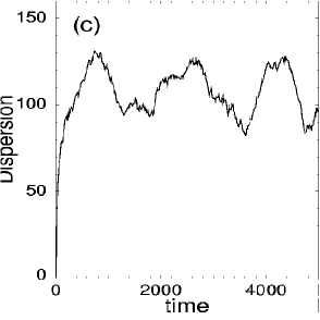
FIG. 18.: Time-evolution of the dispersion $\sigma=\sigma(m)$, where $m=t/T$, for three values of the wave amplitudes: (a) $\epsilon=0.05$, (b) $\epsilon=0.5$, (c) $\epsilon=7.6$, and for $h=0.5$, $\ell=5$, $\delta=0$.

In order to illustrate a non-monotonic character of localization of the QGS as a function of the wave amplitude at small $\epsilon$, we computed the dynamics of the quantum state initially concentrated on the ground state of the harmonic oscillator, $C_{n}(0)=\delta_{n,0}$, using Eq (31). Time-evolution of the dispersion,

$$\sigma(mT)=\sqrt{\sum_{n}|C_{n}(mT)|^{2}(n-\bar{n}(mT))^{2}},$$ (35)

where $\bar{n}(mT)=\sum_{n}|C_{n}(mT)|^{2}n$ is the average, is presented in Figs. 18 (a) - 18 (c), for three values of $\epsilon$. When the wave amplitude, $\epsilon$, is small (Fig. 18 (a)), a small part of the wave packet can propagate to large values of $n$ due to effect of diffusion via the separatrices as shown in Fig. 19 (a). Similar tunneling effect of the wave packet between the resonance cells via the separatrices was explored in Ref. [7] In spite of a small probability of tunneling to other cells, contribution of this part to the dispersion, $\sigma$, is significant because it is proportional to $(n-\bar{n})^{2}$, where $n-\bar{n}\gg 1$. At $\epsilon=0.5$ the separatrix QE states are destroyed by chaos, as shown in Fig. 17 (b), and QGS becomes more localized (see Fig. 19 (b)). This leads to a significant decrease of $\sigma$ in Fig. 18 (b) in comparison with the case of small $\epsilon$, shown in Fig. 18 (a). Further increase of $\epsilon$, up to the value $\epsilon=7.6$, results in delocalization of the QGS, as shown in Fig. 19 (c), and the dispersion, $\sigma=\sigma(mT)$, in Fig. 18 (c) becomes large again.

     

FIG. 19.: Probability distribution in the system with initial condition $C_{n}(0)=\delta_{n,n_{0}}$ and (a) $\epsilon=0.05$, $mT=3\times 10^{5}T$; here $|C_{0}|^{2}=0.746$, (b) $\epsilon=0.5$, $mT=10^{4}T$; $|C_{0}|^{2}=0.982$, (c) $\epsilon=7.6$, $mT=5000T$; $|C_{0}|^{2}=0.137$, $|C_{1}|^{2}=0.423$. The boundaries of quantum cells (quantum separatrices) are marked by arrows; $h=0.5$, $\ell=5$, $\delta=0$.

Comparison of Figs. 19 (a) and 19 (c) allows us to conclude that delocalization of the QGS at very small, and at large values of $\epsilon$ is of a different nature. In the former case, the diffusion is caused by the separatrix QE states. These states are the quantum objects because they are delocalized, and provide tunneling between the resonant cells. [7] As a consequence of the quantum nature of the separatrix QE states, increase of the dimensionless Planck constant, $h$, leads to delocalization of the separatrix QE states and decrease of localization of QGS at small $\epsilon$, shown in Fig. 16. On the other hand, when $\epsilon$ is large we observe delocalization caused by chaos, which is manifested in the irregular form of the probability distribution, shown in Fig. 19 (c).

As follows from Fig. 16, in order to make the QGS more stable at small $\epsilon$ one should decrease the Planck constant, $h$. A plot of the dispersion, $\sigma$, versus time for $h=0.1$ is presented in Fig. 20 (a). The system remains in the ground state with the probability $P_{0}=0.996$. However the dispersion is still large enough because the particle can propagate with small probability to the levels with large $n\gg 1$, due to the diffusion via the separatrices which can be seen from the plot of the probability distribution presented in Fig. 20 (b).

Another way to increase the stability of the ground state at small $\epsilon$, is to destroy the separatrix QE functions by choosing the non-resonant value of the wave frequency, so that $\delta=\ell-\Omega/\omega\neq 0$. For a non-resonant case ($\delta=0.01$), the plot of the dispersion as a function of time is presented in Fig. 21 (a), and the probability distribution at time $m=t/T=3\times 10^{6}$ is illustrated in Fig. 21 (b). One can see from Fig 21 (a) that introducing a detuning, $\delta\neq 0$, results in considerable improvement of the stability of the QGS in comparison with the case of the exact resonance, illustrated in Fig. 18 (a). Thus, in order to make the ground state more stable at small values of $\epsilon$ one must detune the system from the exact resonance.

The minimal value of detuning, $\delta$, required to destroy the separatrix structure, and to make the ground state more stable, can be estimated from the quantum equations of motions in the resonance approximation (27). The term, proportional to $\delta n$ destroys the separatrix QE states as shown in Ref.[6] This term becomes significant when it becomes of the order of the relation, $\epsilon/h$. On the other hand, the separatrix QE function must, at least, occupy the two separatrices. Thus, we can estimate the number, $n=n_{\delta}$, of the oscillator’s state at which the separatrix structure is destroyed, namely $n_{\delta}=\epsilon/\delta h$. The separatrix QE functions decay exponentially with increasing $n$ in the region $n>n_{\delta}$.[6] For the parameters in Fig. 21, $n_{\delta}=50$, which is much less than the position of the first separatrix $n_{1}=385$ shown in Fig. 20 (b) by arrow. So, the separatrix QE states at these parameters do not exist, and we do not observe tunneling from the QGS to other resonance cells.

    

FIG. 20.: (a) Time-evolution of the dispersion, $\sigma=\sigma(m)$, where $m=t/T$, and (b) probability distribution at time $m=3\times 10^{6}$ for small value of $h$, $\delta=0$, $h=0.1$, $\epsilon=0.05$

    

FIG. 21.: (a) Time-evolution of the dispersion $\sigma=\sigma(m)$, where $m=t/T$, and (b) probability distribution at time $m=3\times 10^{6}$ for the near resonance case, $\delta=0.01$; $h=0.1$, $\epsilon=0.05$

Decreasing the value of $\epsilon$, in the near resonance case, makes the QGS more stable. Unlike the near resonance case, in the case of the exact resonance, a stability of the QGS at $\epsilon\ll 1$ is independent of the wave amplitude, because in this case the localization properties of the QGS are defined by the structure of separatrix QE function, which in the resonance approximation (when $\epsilon$ is small) is independent of $\epsilon$.[6] One can see from a comparison of Fig. 21 (a) with Fig. 20 (a) ($h=0.1$, $\epsilon=0.05$) that the dispersion in the near resonance case (Fig. 21 (a)) is much less than that in the exact resonance case (Fig. 20 (a)), in spite of the probability to stay in the ground state, $P_{0}$, for these two cases does not differ significantly ($P_{0}=0.99897$ at $\delta=0.01$ and $P_{0}=0.996$ at $\delta=0$). The reason is that the dynamics in the exact resonance case is mainly determined by the separatrix QE function, and in this case there is a small probability for particle to tunnel to the high oscillator levels with $n\gg 1$, as shown in Fig. 20 (b).

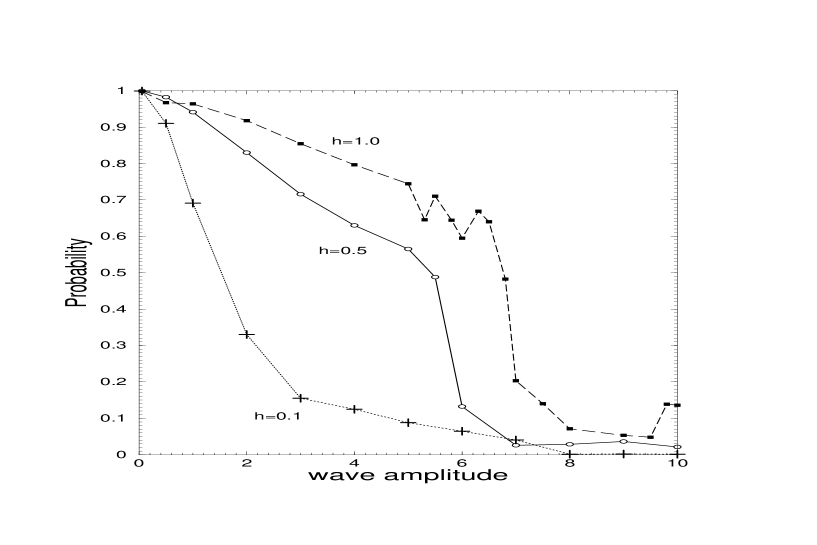
FIG. 22.: The same as in Fig. 16, but for the near resonance case, $\delta=0.01$.

When the wave amplitude $\epsilon$ increases, the condition $\delta\neq 0$ becomes less significant. This can be explained by less influence of the term proportional to $\delta$ on the dynamics in comparison with influence of the wave with the amplitude $\epsilon$ in the region where the value of $kr$ is relatively small (see the classical Hamiltonian in Eqs. (6), (7), (9) and quantum Eq. (27)). In Fig. 22 we plot the function $P_{0}=P_{0}(\epsilon)$ for the near resonance case. In Figs. 23 (a) - 23 (c) we compare the results for the exact resonance case ($\delta=0$) with those for the near resonance case, when $\delta=0.01$ and $\delta=0.1$. One can see from these figures that the dynamics in the vicinity of the QGS in the near resonance case is similar to that in the exact resonance case, except for the region of small $\epsilon$, which was discussed above.

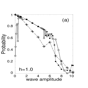
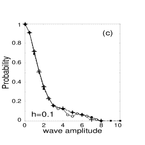
FIG. 23.: Plot of $P_{0}$ versus $\epsilon$ for the exact resonance case, when $\delta=0$ (solid line and open circles), and two curves for the near resonance cases: $\delta=0.01$ (dashed line and filled squares), $\delta=0.1$ (dot-dashed line and crosses); $\ell=5$, (a) $h=1$, (b) $h=0.5$, (c) $h=0.1$.

In the quantum case, similar to the classical one, at very small $\epsilon$ and finite $\delta$, there always exists the QGS QE state at any $\ell$ including the cases $\ell=1$ and $\ell=2$. In Fig. 24 we present a plot $P_{0}=P_{0}(\epsilon)$ for the cases $\ell=1$ and $\ell=2$ when $\delta=0.1$ and $h=0.5$. As one can see from Fig. 24 the QGS QE state in these two cases becomes unstable at considerably less values of $\epsilon$ than that in the case $\ell=5$ in Fig. 23, which corresponds to the classical dynamics in Figs. 8 - 10. In the case $\ell=1$ the stable point shifts down from the region $X=0,\,P=0$ in Figs. 8 (a)- 8 (c), and in the case $\ell=2$ the stable point at $\epsilon\approx 0.2$ becomes unstable (see Figs. 9 (a), 9 (b)) and 10). The quantum manifestation of this process is a rapid decay of the value of $P_{0}$ in the region $\epsilon\geq 0.2$ in Fig. 24.

In conclusion, the classical dynamics in the vicinity of the point ($x=0,\,p=0$) in the classical phase space and quantum dynamics in the vicinity of the ground state of the harmonic oscillator in a field of a monochromatic wave, is explored. Both resonance and near resonance cases are analyzed. It is shown that at small $\epsilon$ and finite detuning from the resonance, $\delta$, the quantum ground state is always stable. In the case $\delta=0$, the dynamics is unstable for the resonance numbers $\ell=1,2$. Stability of the classical dynamics in the central cell and stability of the quantum dynamics near the ground state of the harmonic oscillator under the influence of chaos is analyzed. It is shown, that under certain conditions ($\ell>2,\,\delta=0,\,\epsilon\ll 1,\,h\sim 1$) the presence of chaos makes the quantum ground state more localized. Increase of the quantum parameter, $h$, at intermediate values of $\epsilon$, enhances localization of the QGS considerably. Experimental observation of discussed results in the system of an ion trapped in a linear ion trap and interacting with laser fields represents a significant interest for understanding the stability properties of this system.

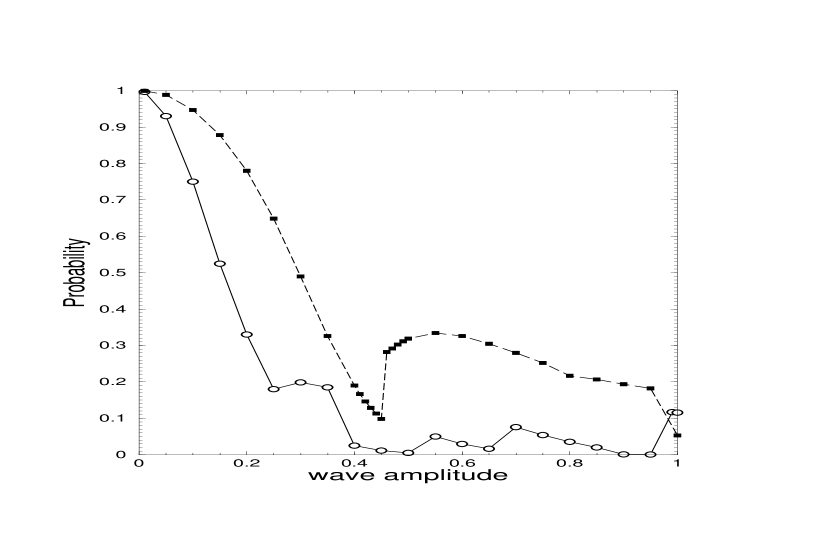
FIG. 24.: Plot $P_{0}=P_{0}(\epsilon)$ for the resonance numbers $\ell=1$ (open circles and solid line) and $\ell=2$ (filled squares and dashed line) in the near resonance case, $\delta=0.1$; $h=0.5$.

V Acknowledgments

We are thankful to R.J. Hughes and G.D. Doolen for useful discussions. This work was supported by the National Security Agency, and by the Department of Energy under the contract W-7405-ENG-36. Work of D.I.K. was partly supported by Russian Foundation for Basic Research (Grants No. 98-02-16412 and 98-02-16237).

REFERENCES

- [1] R.J. Hughes, D.F.V. James, J.J. Gomez, M.S. Gulley, M.H. Holzscheiter, P.G. Kwiat, S.K. Lamoreaux, C.G. Peterson, V. D. Sandberg, M.M. Schauer, C.M. Simmons, C.E. Thorburn, D. Tupa, P.Z. Wang and A.G. White, Fortschritte der Physik, 46, 329 (1998).
- [2] G.P. Berman, G.D. Doolen, R. Mainieri and V.I. Tsifrinovich, Introduction to Quantum Computers, World Scientific Publishing Company, Singapore, 1998.
- [3] G.P. Berman, D.F.V. James, R.J. Hughes, M.S. Gulley, M.H. Holzscheiter, G.V. López, quant-ph/9903063.
- [4] G.M. Zaslavsky, R.Z. Sagdeev, D.A. Usikov, and A.A. Chernikov, Weak Chaos and Quasiregular Patterns, (Cambridge Univ. Press, Cambridge, 1991)
- [5] A.J. Lichtenberg and M.A. Lieberman, Regular and Stochastic Motion, (Springer, New York, 1983).
- [6] V.Ya. Demikhovskii, D.I. Kamenev, and G.A. Luna-Acosta, Phys. Rev. E, 52, (1995) 3351.
- [7] V.Ya. Demikhovskii, D.I. Kamenev, and G.A. Luna-Acosta, Phys. Rev. E, 59, (1999) 294.
- [8] N.W. McLachlan, Theory and application of Mathieu functions, (Oxford University Press, Oxford, 1947).
- [9] L.D. Landau, E.M. Lifshits, Mechanics, (Moscow, 1958) (in Russian).
- [10] G.P. Berman, A.R. Kolovsky, G.M. Zaslavsky, Phys. Lett. A, 111, (1982) 17.
- [11] G.P. Berman, A.R. Kolovsky, Sov. Phys. Usp., 35 (1992) 303.
- [12] L.E. Reichl and W.A. Lin, Phys. Rev. A, 40, (1989) 1055.
- [13] G.P. Berman, O.F. Vlasova, F.M. Izrailev, Sov. Phys. JETP, 66, (1987) 269.
- [14] G.P. Berman, V.Ya. Demikhovskii, D.I. Kamenev, quant-ph/9906079.
- [15] V.Ya. Demikhovskii, D.I. Kamenev, Phys. Lett. A, 228, (1997) 391.