Generalized Amplitude Truncation of Gaussian $1/f^{\alpha}$ noise

Abstract

We study a kind of filtering, an amplitude truncation with upper and lower truncation levels $x_{\rm{max}}$ and $x_{\rm{\min}}$. This is a generalization of the simple transformation $y(t)=\rm{sgn}[\it{x(t)}]$, for which a rigorous result was obtained recently. So far numerical experiments have shown that a power law spectrum $1/f^{\alpha}$ seems to be transformed again into a power law spectrum $1/f^{\beta}$ under rather general condition for the truncation levels. We examine the above numerical results analytically. When $1<\alpha<2$ and $x_{\rm{max}}=-x_{\rm{min}}=a$, the transformed spectrum is shown to be characterized by a certain corner frequency $f_{\rm c}$ which divides the spectrum into two parts with different exponents. We derive $f_{\rm c}$ depending on $a$ as $f_{\rm c}\sim a^{-2/(\alpha-1)}$. It turns out that the output signal should deviate from the power law spectrum when the truncation is asymmetrical. We present a numerical example such that $1/f^{2}$ noise converges to $1/f$ noise by applying the transformation $y(t)=\rm{sgn}[\it{x(t)}]$ repeatedly.

Department of Physics, Tokyo Metropolitan University, Minami-Ohsawa, Hachioji, Tokyo 192-0397, Japan

KEYWORDS: 1/f fluctuation, nonlinear transformation, filtering, power law

§1 Introduction

$1/f$ noise whose power spectrum is inversely proportional to the frequency $f$ has been observed in a variety of systems, since it was first discovered in current fluctuations of a vacuum tube (see ref. 1 and references therein). Sometimes $1/f^{\alpha}$ noise with the exponent $\alpha$ not close to $1$ but between $0$ and $2$ is also referred to as ‘$1/f$ noise’[2, 3]. When this extended definition is applied, ‘$1/f$ noise’ is more widely observed[4].

It should be noted that the integral $\int_{0}^{\infty}f^{-\alpha}df$ diverges for all $\alpha$. Therefore, if the process is stationary, which is usually a reasonable assumption, a low or high frequency cut off should exist corresponding to $\alpha\geq 1$ or $0\leq\alpha\leq 1$, respectively. Or equivalently, the value of $\alpha$ cannot be constant: $\alpha$ should become smaller (larger) than unity in a low (high) frequency range. The power law behavior involves several difficulties. The autocorrelation function of $1/f^{\alpha}$ noise with $\alpha<1$ decays very slowly (power law decay, see eq. (LABEL:eqn:incor1b) and Fig. 1(a)) especially when $\alpha$ is close to unity, unless there is another low frequency cut off $f_{0}$ so that the spectrum becomes white ($\alpha=0$) in a range $f\ll f_{0}$. It often happens that the cut off frequency $f_{0}$ is extremely low or not observed during the practical observation time.[4, 5] One of the difficulties is to explain a long time scale $\sim 1/f_{0}$ from any realistic model. Another problem is the value of the exponent which largely deviates from $2$. The exponent $\alpha=2$ is most naturally expected in nonstationary processes. Random walk in $n$-dimensional space yields $1/f^{2}$ spectrum. Also, a Lorentzian spectrum $(f^{2}+f_{0}^{2})^{-1}$ looks as $1/f^{2}$ when the observation time is not long enough: $f\gg f_{0}$. Lorentzian spectrums are obtained from Debye-type relaxation processes, which occur most commonly. A randomly amplified Langevin system which has a power law distribution function also leads to a Lorentzian spectrum,[6] even though the process is nonstationary so that the Wiener-Khintchine theorem does not hold. Then what mechanism could exist that would reduce the value of $\alpha$ from $2$? The present work relates to this second problem. We shall investigate, by generalizing a previous theory[1], how Gaussian $1/f^{\alpha}$ noise is affected by a kind of filtering, an amplitude truncation.

In the previous paper, a simple dichotomous transformation defined by $y(t)=\rm{sgn}[\it{x(t)}]$ for Gaussian $1/f^{\alpha}$ noise was studied in detail and a rigorous result for transformation properties was obtained[1]. When a Gaussian noise $x(t)$ with a power law spectrum $1/f^{\alpha}$ is filtered by this transformation, power spectral density (PSD) of the output noise $y(t)$ obeys again a power law $1/f^{\beta}$. The exponent $\beta$ is derived as $\beta=\alpha$ for $0<\alpha\leq 1$, and $\beta=(\alpha+1)/2$ for $1\leq\alpha<2$.

The present paper deals with a more general amplitude truncation

$$y(t)=\left\{\begin{array}[]{ll}x_{\rm{min}}&\mbox{ if }\;\;\;x(t)\leq x_{\rm{min}}\mbox{, }\\ x_{\rm{max}}&\mbox{ if }\;\;\;x(t)\geq x_{\rm{max}}\mbox{, }\\ x(t)&\mbox{ otherwise, }\end{array}\right.$$ (1)

for Gaussian $1/f^{\alpha}$ noise. The transformation $y(t)=\rm{sgn}[\it{x(t)}]$ is equivalent to the situation $x_{\rm{max}}=-x_{\rm{min}}\ll 1$ in eq. (1), namely, the dichotomous transformation is a special case of eq. (1). So far numerical experiments have shown[7, 8] that a power law spectrum $1/f^{\alpha}$ seems to be transformed again into a power law spectrum $1/f^{\beta}$ under rather general condition for the truncation levels $x_{\rm{min}}$ and $x_{\rm{max}}$. However, the numerical results are not always clear, so that we will investigate analytically the above amplitude truncation to know how $\beta$ depends on the levels as well as $\alpha$ and when the output signal deviates from the power law spectrum.

The rest of the present paper is organized as follows. In the next section, we briefly review and reinterpret the recent result for the dichotomous transformation. In §3, we extend our study for the symmetrical truncation with finite levels : $x_{\rm{max}}=-x_{\rm{min}}=a$ in (1). We consider the asymmetrical truncation in §4. It will be shown how PSD of the output signal deviates from the power law. In §5, we present a numerical example such that $1/f^{2}$ noise converges to $1/f$ noise by applying the dichotomous transformation repeatedly. The last section is devoted to summary and discussions.

§2 Dichotomous Transformation

The dichotomous transformation is defined by

$$y(t)=\rm{sgn}[\mit x(t)]=\left\{\begin{array}[]{ll}-1&\mbox{ if }\;\;\;x(t)\leq 0\mbox{ , }\\ +1&\mbox{ if }\;\;\;x(t)>0\mbox{ , }\\ \end{array}\right.$$ (3)

where $x(t)$ is an input noise with zero mean and $y(t)$ is an output noise. This is a special case of the amplitude truncation (1) and was investigated in detail in ref. 1. It turned out that when the transformation (3) is applied to a Gaussian $1/f^{\alpha}$ noise $x(t)$, then the output noise $y(t)$ exhibits a power law spectrum $1/f^{\beta}$. The exponent $\beta$ was derived as $\beta=\alpha$ for $0<\alpha\leq 1$, and $\beta=(\alpha+1)/2$ for $1\leq\alpha<2$. As will be shown below, a key to understand this result is a transformation property of the correlation function $R(t)$ (eq. (9)).

The correlation function of the output signal $y(t)$ is obtained from eq. (3) as

$$R_{y}(t) \equiv \langle y(t_{0})y(t_{0}+t)\rangle$$ (4)

$$= 1\cdot P\left(y(0)y(t)=1\right)+(-1)\cdot P\left(y(0)y(t)=-1\right)$$

$$= P\left(x(0)x(t)>0\right)-P\left(x(0)x(t)<0\right)$$

$$= 2\cdot P\left(x(0)x(t)>0\right)-1\mbox{ , }$$

where $P(.)$ stands for the probability that the condition of the argument is satisfied. In the above, we have assumed a stationary process for the input noise, which leads to a stationary process for the output one. We can therefore apply the Wiener-Khintchine theorem to both input and output noises. We also assume that the process for the input noise is correlated Gaussian[9]. That is, the joint probability is given by

$$P(x(t_{0}),x(t_{0}+t)) = P(x(0),x(t))$$ (5)

$$= \frac{1}{A_{0}}\exp[-(x^{2}-2cxy+y^{2})/B]$$

$$\equiv f(x,y,c)\mbox{ , }$$

where,

$$\left\{\begin{array}[]{ll}x\equiv x(0)\mbox{ , }\\ y\equiv x(t)\mbox{ , }\\ c\equiv R_{x}(t)\mbox{ , }\\ A_{0}\equiv 2\pi R_{x}(0)\sqrt{1-c^{2}}\mbox{ , }\\ B\equiv 2R_{x}(0)(1-c^{2})\mbox{ , }\\ \end{array}\right.$$ (6)

and

$$R_{x}(t)\equiv\langle x(t_{0})x(t_{0}+t)\rangle$$ (7)

is the correlation function of $x(t)$.

The probability $P(xy>0)$ is calculated from eq. (5) as

$$P(xy>0) = \int_{0}^{\infty}dx\int_{0}^{\infty}dyf(x,y,c)$$ (8)

$$+\int_{-\infty}^{0}dx\int_{-\infty}^{0}dyf(x,y,c)$$

$$= \frac{1}{2}+\frac{1}{\pi}\arcsin[R_{x}(t)]\mbox{ . }$$

Thus we obtain the relation between the input and output correlation functions as

$$R_{y}(t)=\frac{2}{\pi}\arcsin[R_{x}(t)]\mbox{ . }$$ (9)

The previous result for the exponent $\beta$ can easily be understood qualitatively if we note the approximated expression for (9):

$$\mbox{ when }|R_{x}(t)|\ll 1\mbox{ , }\;\;\;\;\;\;\;\;R_{y}(t)\propto R_{x}(t);$$ (10)

$$\mbox{ when }|1-R_{x}(t)|\ll 1\mbox{ , }\;\;R_{y}(t)\propto\mbox{const.}-(1-R_{x}(t))^{\frac{1}{2}}\mbox{ . }$$ (11)

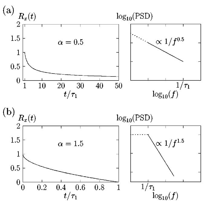
Figure 1: Correlation function $R_{x}(t)$ of a $1/f^{\alpha}$ noise. (a) $0<\alpha<1$: eqs. (1). (b) $1<\alpha<2$: eqs. (1).

First we explain $\beta=\alpha$ for $0<\alpha<1$. When PSD for low frequencies obeys the power law as $\sim f^{-\alpha}$ with $0<\alpha<1$, the corresponding correlation function $R_{x}(t)$ should be $R_{x}(t)\sim t^{\alpha-1}$ for large $t$ values[1, 10]. Let us consider a system whose characteristic time scale is $\tau_{1}$. Then, by assuming $R_{x}(t)$ as R_x(t)&= 1                  for    t/τ_1 ≤1 ,
eqn:incor1b R_x(t)= (t/τ_1)^α-1     for    t/τ_1 ≥1 , the PSD is $\sim(\tau_{1}f)^{-\alpha}$ for low frequencies: $0<f\ll 1/\tau_{1}$. The relation (10) can be used to obtain $R_{y}(t)$ for large $t$: $t/\tau_{1}\gg 1$, because $R_{x}(t)$ is small. This is why the same exponent $\beta=\alpha$ is obtained for $0<\alpha<1$.

The case $1<\alpha<2$ can also be understood qualitatively. Let us assume the correlation function as eqn:incor2 R_x(t)&= 1-(t/τ_1)^α-1     for     t/τ_1 ≤1 ,
eqn:incorb R_x(t)= 0                        for     t/τ_1 ≥1 . The above correlation function yields a white spectrum if the observation time $t$ is long enough: $t\gg\tau_{1}$, i.e., $f\ll 1/\tau_{1}$. Naturally we are interested in the situation in which the characteristic time scale $\tau_{1}$ is very long. The power law, eq. (LABEL:eqn:incor2) again leads to the power law spectrum $S_{x}(f)\propto(\tau_{1}f)^{-\alpha}$ for a wide range: $f\gg 1/\tau_{1}$[1]. Note that if $\tau_{1}$ is very long, the lower limit $1/\tau_{1}$ can be small and the power law $\sim f^{-\alpha}$ holds practically in a wide range of low frequencies. When time $t$ is long enough but satisfies $t\ll\tau_{1}$, the approximation (11) can be used for $R_{y}(t)$:

$$R_{y}(t) \propto \mbox{ const.}-(t/\tau_{1})^{\frac{\alpha-1}{2}}$$ (12)

$$\equiv \mbox{ const.}-(t/\tau_{1})^{\beta-1}\mbox{ . }$$

Corresponding to the above $R_{y}(t)$, the PSD is obtained as $\sim f^{-\beta}$, where $\beta=(\alpha+1)/2$.

§3 Symmetrical Truncation with Finite Levels

In this section we generalize the results obtained in the above. Suppose that a Gaussian $1/f^{\alpha}$ noise with zero mean is transformed by a symmetrical truncation with finite levels $x_{\rm{max}}=-x_{\rm{min}}\equiv a$. Let us define a typical time scale $\tau_{\rm c}$ in which the noise signal passes between the two truncation levels. In a high frequency range $f\gg f_{\rm c}\equiv 1/\tau_{\rm c}$, PSD of the truncated noise is mainly determined by the behavior of the noise between the two levels. On the other hand, in a low frequency range $f\stackrel{{\scriptstyle\displaystyle<}}{{\raisebox{-4.30554pt}{$\sim$}}}f_{\rm c}$ (corresponding to a long-term observation), PSD of the output signal should have a similar PSD to that obtained by the dichotomous transformation. Therefore, for $0<\alpha<1$, the same exponent $\beta=\alpha$ is expected both in high ($f_{\rm c}\stackrel{{\scriptstyle\displaystyle<}}{{\raisebox{-4.30554pt}{$\sim$}}}f\ll 1/\tau_{1}$) and low ($f\stackrel{{\scriptstyle\displaystyle<}}{{\raisebox{-4.30554pt}{$\sim$}}}f_{\rm c}$) frequency ranges.

In contrast, when $1<\alpha<2$, PSD is divided into two parts by a corner frequency $f_{\rm c}$: $\beta=\alpha$ for a high frequency range ($f\stackrel{{\scriptstyle\displaystyle>}}{{\raisebox{-4.30554pt}{$\sim$}}}f_{\rm c}$) and $\beta=(\alpha+1)/2$ for a low frequency range ($1/\tau_{1}\ll f\stackrel{{\scriptstyle\displaystyle<}}{{\raisebox{-4.30554pt}{$\sim$}}}f_{\rm c}$). A typical PSD of a truncated signal for $\alpha=2$ is shown in Fig. 2.

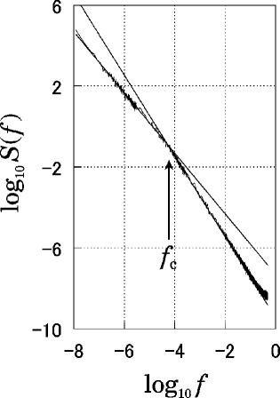
Figure 2: PSD of the truncated signal for $\alpha=2$. The PSD is obtained by averaging over $40$ samples. PSDs in three frequency ranges are composed. Straight lines are $S(f)\propto f^{-2}$ and $\propto f^{-1.5}$

The aim in this section is to derive the dependence of $f_{\rm c}$ upon the truncation level $a$. The transformation is expressed as

$$y(t)=\left\{\begin{array}[]{ll}x(t)&\mbox{ if }\;-a\leq x(t)\leq a\mbox{, }\\ a\cdot\rm{sgn}[\mit x(t)]&\mbox{ otherwise, }\end{array}\right.$$ (1)

where $x(t)$ is a correlated Gaussian noise with zero mean.

As in the previous section, the joint probability (5) yields the correlation function of the output signal as

$$R_{y}(t) = 2\cdot a^{2}(I(c)-I(-c))+2\cdot(J(c)-J(-c))$$ (2)

$$+4\cdot a(K(c)-K(-c))\mbox{ , }$$

where

$$I(c)\equiv\int_{a}^{\infty}dx\int_{a}^{\infty}dyf(x,y,c)\mbox{ , }$$

$$J(c)\equiv\int_{0}^{a}dx\int_{0}^{a}dy\;xyf(x,y,c)\mbox{ , }$$

$$K(c)\equiv\int_{a}^{\infty}dx\int_{0}^{a}dy\;yf(x,y,c)\mbox{ . }$$

If we assume $a\ll 1$, $I(c)$, $J(c)$ and $K(c)$ can be expanded with respect to $a$ as

$$I(c) = \frac{1}{4}[1+\frac{2}{\pi}\arcsin(c)]-a\frac{\sqrt{B\pi}}{A_{0}}-a^{2}\frac{c-1}{A_{0}}+O(a^{3})\mbox{ , }$$

$$J(c) = a^{4}\frac{6}{4!A_{0}}+O(a^{5})\mbox{ , }$$

$$K(c) = a^{2}\frac{\sqrt{B\pi}}{2!2A_{0}}+a^{3}\frac{2c-3}{3!A_{0}}+O(a^{4})\mbox{ . }$$ (3)

Substitution of Eq. (3) into (2) leads to the correlation function of the output signal as

$$R_{y}(t) = 2a^{2}\{\frac{1}{\pi}\arcsin(c)-2\cdot\frac{ca^{2}}{2\pi\sqrt{1-c^{2}}}+\cdots\}$$

$$+4a\{\frac{ca^{3}}{3\pi\sqrt{1-c^{2}}}+\cdots\}$$

$$= a^{2}\{\frac{2}{\pi}\arcsin(c)-\frac{2ca^{2}}{\pi\sqrt{1-c^{2}}}+\frac{4ca^{2}}{3\pi\sqrt{1-c^{2}}}+\cdots\}\mbox{ . }$$

Since we are considering the case of $1<\alpha<2$ , we substitute $c\equiv R_{x}(t)=1-t^{\alpha-1}$ (eq. (LABEL:eqn:incor2)) into the above. The correlation function is thus obtained as

$$R_{y}(t) \simeq a^{2}\{1-\frac{2\sqrt{2}}{\pi}t^{(\alpha-1)/2}$$ (4)

$$-a^{2}\frac{\sqrt{2}}{3\pi}t^{-\frac{\alpha-1}{2}}+\cdots\},$$

for $t\ll 1$. Here and hereafter, the dimensionless time $t/\tau_{1}$ is replaced by $t$ for simplicity. Thus $t\ll 1$ actually means $t\ll\tau_{1}$. If $a$ is small enough and/or $t$ is not so small so that the third term in the braces in (4) can be neglected, $R_{y}(t)$ reduces to eq. (12). As $t$ decreases, the third term grows and becomes comparable to the second term. In other words, the perturbative expansion (4) breaks down when $t^{(\alpha-1)/2}\sim a^{2}t^{-(\alpha-1)/2}$ i.e. $t\sim a^{2/(\alpha-1)}$. This means that the corner frequency $f_{\rm c}$ depends on the truncation level $a$ as

$$f_{\rm c}\sim a^{-2/(\alpha-1)}.$$ (5)

For a long-term observation, i.e., $1\gg t\stackrel{{\scriptstyle\displaystyle>}}{{\raisebox{-4.30554pt}{$\sim$}}}a^{2/(\alpha-1)}$ (which corresponds to $1\ll f\stackrel{{\scriptstyle\displaystyle<}}{{\raisebox{-4.30554pt}{$\sim$}}}f_{\rm c}$), the exponent $\beta$ of the PSD becomes $\beta=(\alpha+1)/2$ because (4) reduces to (12). For a high frequency range: $f\stackrel{{\scriptstyle\displaystyle>}}{{\raisebox{-4.30554pt}{$\sim$}}}f_{\rm c}$, the same exponent $\beta=\alpha$ as the input signal is expected by the reason mentioned already, although the correlation function of the form $R_{y}(t)\sim\mbox{const.}-t^{\alpha-1}$ (which corresponds to the PSD$\sim f^{-\alpha}$) cannot be obtained from any correction terms added to (4) because the perturbative expansion has broken down. One can see in Fig. 2 that the PSD obtained from the numerical simulation is really composed of two power law spectra separated by the corner frequency $f_{\rm c}$.

The scaling property of eq. (5) can also be suggested from the following self-affine character of the signal from the fractional Brownian motion:[11]

$$\langle x(t)^{2}\rangle\sim t^{2H}.$$ (6)

It is well known that if a signal satisfies the scaling relation (6), then its PSD is $1/f^{\alpha}$ with $\alpha=2H+1$ where $\alpha\geq 0$[11]. The above self-affine character yields

$$\sqrt{\langle x(t)^{2}\rangle} = \sqrt{\langle x(a^{-\frac{1}{H}}a^{\frac{1}{H}}t)^{2}\rangle}$$ (7)

$$\propto \frac{1}{a}\sqrt{\langle x(a^{\frac{1}{H}}t)^{2}\rangle}.$$

This means that if the truncation levels are changed from $\pm U$ to $\pm aU$ and the time is changed from $t$ to $a^{1/H}t$ simultaneously, the structure of the noise is invariant. Then the corner frequency changes from $f_{\rm c}$ to $a^{-(1/H)}f_{\rm c}=a^{-2/(\alpha-1)}f_{\rm c}$. This coincides with the result obtained from the perturbation method; the present argument can be applicable even for large $a$ values.

To confirm $a$-dependence of $f_{\rm c}$, eq. (5), we performed a numerical simulation for $\alpha=2$ by varying the truncation level $a$ in eq. (1). For each $a$ value, a PSD $S(f)$ was obtained by averaging over $40$ samples. Then $\log S(f)$ was fitted to the line $F(f)=(-1.5\log f+1.5\log f_{\rm c}+A)\Theta(\log f_{\rm c}-\log f)+(-2.0\log f+2.0\log f_{\rm c}+A)\Theta(\log f-\log f_{\rm c})$ where $\Theta(x)$ is a Heaviside function with $\Theta(0)=1/2$. The result is shown in Fig. 3. Agreement between the theoretical line: $f_{\rm c}\propto a^{-2}$ and the numerical result is tolerable.

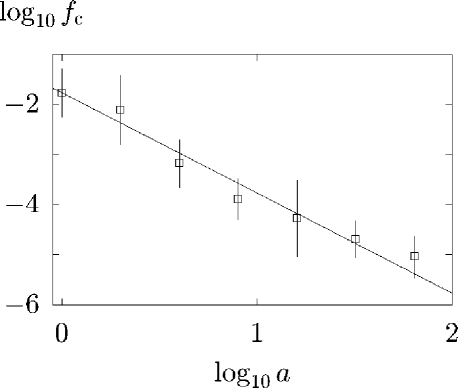
Figure 3: Log-log plot of the corner frequency $f_{\rm c}$ vs the truncation level $a$ for $\alpha=2$. The straight line is $f_{\rm c}\propto a^{-2}$.

§4 Asymmetrical Truncation

We consider the simplest case, i.e., the following asymmetrical dichotomous transformation:

$$y(t)=\rm{sgn}[\mit x(t)-a]=\left\{\begin{array}[]{ll}+1&\mbox{ if }\;\;\;x(t)\geq a\mbox{, }\\ -1&\mbox{ if }\;\;\;x(t)<a\mbox{. }\end{array}\right.$$ (1)

The input signal is a Gaussian $1/f^{\alpha}$ noise with zero mean, and the condition $0<\alpha<1$ is assumed here.

Figure  4 illustrates the PSD of the output signal obtained by eq. (1) for $\alpha=0.8$ and $a=0,\sigma,2\sigma$, where $\sigma$ is the standard deviation of the input signal. It is unclear from these numerical results whether the PSD obeys the power law or not.

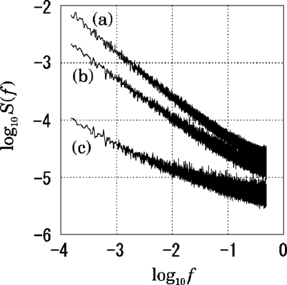
Figure 4: Output PSDs obtained from the asymmetric transformation (1) where the exponent of the input noise is $\alpha=0.8$. Each PSD was obtained by averaging over 40 samples. (a), (b), and (c) correspond to the truncation level $a=0$, $\sigma$ and 2$\sigma$, respectively, where $\sigma$ is the standard deviation of the input signal.

Note that the mean value of the output signal is finite:

$$\langle y(t)\rangle = \int_{-\infty}^{\infty}\mbox{sgn}[x-a]f(x)dx$$ (2)

$$= -2\int_{0}^{a}f(x)dx\equiv\bar{y}\mbox{ , }$$

where $f(x)$ is the Gaussian distribution function for the input signal:

$$f(x)=\frac{1}{\sqrt{2\pi R_{x}(0)}}\exp\left[-\frac{x^{2}}{2R_{x}(0)}\right]\mbox{ . }$$ (3)

The correlation function of $y(t)$ is thus given by

$$R_{y}(t) = \langle(y(t_{0})-\bar{y})(y(t_{0}+t)-\bar{y}\rangle$$ (4)

$$= \langle y(t_{0})y(t_{0}+t)\rangle-(\bar{y})^{2}$$

$$= 2P((x(0)-a)(x(t)-a)>0)-1-(\bar{y})^{2}\mbox{ . }$$ (5)

The probability $P((x(0)-a)(x(t)-a)>0)$ is expressed as

$$P((x(0)-a)(x(t)-a)>0)$$ (6)

$$= \bigm{[}2\int_{-\infty}^{\infty}dx\int_{0}^{a}dy+2\int_{a}^{\infty}dx\int_{a}^{\infty}dy\bigm{]}f(x,y,c)\mbox{ , }$$

where $f(x,y,c)$ is the joint probability defined by (5) $\sim$ (7). The first term in (6) depends on $a$ but not on $t$:

$$2\int_{-\infty}^{\infty}dx\int_{0}^{a}dyf(x,y,c)=2\int_{0}^{a}dxf(x)dx=-\bar{y}\mbox{ , }$$ (7)

which yields

$$P((x(0)-a)(x(t)-a)>0)=-\bar{y}+T\mbox{ , }$$ (8)

$$T\equiv 2\int_{a}^{\infty}dx\int_{a}^{\infty}dyf(x,y,c)\mbox{ . }$$ (9)

We calculate $R_{y}(t)$ in two cases $a\ll 1$ and $a\gg 1$. Since $R_{x}(t)$ is assumed as eqs. (1), we set $R_{x}(0)=1$ hereafter.

When $a\ll 1$, $\bar{y}$ is expanded with respect to $a$:

$$\bar{y}=-\frac{2a}{\sqrt{2\pi}}+O(a^{3})\mbox{ . }$$ (10)

The second term $T$ in (8) is similarly expanded as

$$T\equiv\frac{1}{2}+\frac{1}{\pi}\arcsin[c]-\frac{2}{\sqrt{2\pi}}a+\frac{1-c}{\pi\sqrt{1-c^{2}}}a^{2}+\cdots\mbox{ . }$$ (11)

For $t\gg 1$ the correlation function becomes $c\equiv R_{x}(t)=t^{\alpha-1}\ll 1$. Then $T$ can be approximated as

$$T=\frac{1}{2}-\frac{2}{\sqrt{2\pi}}a+\frac{1}{\pi}c+\frac{1}{\pi}(1-c+\frac{1}{2}{c^{2}})a^{2}+O(c^{3})\mbox{ . }$$ (12)

Substituting (8), (10), (12) and $c\equiv t^{\alpha-1}$ into (5), we obtain

$$R_{y}(t) = 2(-\bar{y}+T)-1-\bar{y}^{2}$$

$$\sim \frac{2}{\pi}(1-a^{2})c+\frac{a^{2}}{\pi}c^{2}$$

$$= \frac{2}{\pi}(1-a^{2})t^{\alpha-1}+\frac{a^{2}}{\pi}t^{2(\alpha-1)}\;\;\;\;\;\;\;\mbox{for}\;t\gg 1\mbox{ and }\;a\ll 1\mbox{. }$$ (14)

Equation (14) implies that the correlation function of the output signal obeys a power law $\sim t^{\alpha-1}$ with a small correction term. When the first term in (14) is dominant, i.e. $a^{2}t^{\alpha-1}\ll 1$, the PSD of the output signal turns $f^{-\alpha}$. The condition $a^{2}t^{\alpha-1}\ll 1$ corresponds to $f\ll f_{1}$, where

$$f_{1}\equiv(1/a^{2})^{1/(1-\alpha)}\mbox{ . }$$ (15)

The frequency $f_{1}$ can be very large for small $a$ values because $1-\alpha>0$. The power law spectrum $f^{-\alpha}$ is then observed in a wide range of frequencies.

For $a\gg 1$, an asymptotic expansion of (2) yields

$$\bar{y}=-1+\frac{2}{\sqrt{2\pi}}\exp\left[-\frac{a^{2}}{2}\right]\cdot\bigm{\{}\frac{1}{a}+O(\frac{1}{a^{3}})\bigm{\}}\mbox{ . }$$ (16)

We can calculate $T$ as follows.

$$T = 2\int_{a}^{\infty}\!\!\!\int_{a}^{\infty}\frac{dxdy}{A_{0}}\exp\left[-\frac{x^{2}-2cxy+y^{2}}{B}\right]$$ (17)

$$= 2\frac{1}{A_{0}}\int_{a^{2}}^{\infty}dY\frac{1}{2Y^{\frac{1}{2}}}\exp\left[-\frac{1-c^{2}}{B}Y\right]\int_{a-c\sqrt{Y}}^{\infty}dX\exp\left[-\frac{X^{2}}{B}\right]\mbox{ . }$$

Integrating by parts with respect to the variable $Y$, we obtain

$$T = E+F+G\mbox{ , }$$ (18)

$$E \equiv \frac{B}{A_{0}(1-c^{2})}\frac{1}{a}\exp\left[-\frac{1-c^{2}}{B}a^{2}\right]\int_{(1-c)a}^{\infty}dX\exp\left[-\frac{X^{2}}{B}\right]\mbox{ , }$$

$$F \equiv \frac{B}{A_{0}(1-c^{2})}\int_{a^{2}}^{\infty}dY\frac{-1}{2Y^{\frac{3}{2}}}\exp\left[-\frac{1-c^{2}}{B}Y\right]\int_{a-c\sqrt{Y}}^{\infty}dX\exp\left[-\frac{X^{2}}{B}\right]\mbox{ , }$$

$$G \equiv \frac{B}{A_{0}(1-c^{2})}\int_{a^{2}}^{\infty}dY\frac{c}{2Y}\exp\left[-\frac{1-c^{2}}{B}Y\right]\exp\left[-\frac{(a-c\sqrt{Y})^{2}}{B}\right]\mbox{ . }$$

The second term $F$ in (18) can be neglected because $a\gg 1$. The asymptotic expansion of $E$ is obtained by substituting $X^{2}=x$ and integrating by parts as

$$E=\frac{B^{2}}{2A_{0}(1-c^{2})(1-c)a^{2}}\exp\left[-\frac{2a^{2}(1-c)}{B}\right]+O\left(\frac{1}{a^{4}}\exp\left[-\frac{2a^{2}(1-c)}{B}\right]\right)\mbox{ . }$$ (19)

In a similar manner G is calculated, by substituting $y=(\sqrt{Y}-ca)^{2}$ and integrating by parts, as

$$G=\frac{cB^{2}}{2A_{0}(1-c^{2})(1-c)a^{2}}\exp\left[-\frac{2a^{2}(1-c)}{B}\right]+O\left(\frac{1}{a^{4}}\exp\left[-\frac{2a^{2}(1-c)}{B}\right]\right)\mbox{ . }$$ (20)

Equations (19) and (20) yield

$$T=\frac{(1+c)^{2}}{\pi a^{2}\sqrt{1-c^{2}}}\exp\left[-\frac{a^{2}}{1+c}\right]+O\left(\frac{1}{a^{4}}\exp\left[-\frac{a^{2}}{1+c}\right]\right)\mbox{ . }$$ (21)

Substituting (8), (16), (21) and $c\equiv t^{\alpha-1}$ into (5), we obtain

$$R_{y}(t) \sim \frac{2}{\pi a^{2}}\left[\frac{(1+c)^{2}}{\sqrt{1-c^{2}}}\exp\bigm{[}-\frac{a^{2}}{1+c}\bigm{]}-\exp[-a^{2}]\right]\;\;\mbox{ (for $a^{2}\gg 1$)}$$

$$\sim \frac{2}{\pi a^{2}}\left[(1+2t^{\alpha-1}+\frac{3}{2}t^{2(\alpha-1)})\exp[-a^{2}(1-t^{\alpha-1}+t^{2(\alpha-1)}]-\exp[-a^{2}]\right]\;\;\mbox{ (for $c\ll 1$).}$$

When $a^{2}t^{\alpha-1}\ll 1$, eq. (LABEL:eqn:asabco) reduces to

$$R_{y}(t)\sim\frac{2}{\pi}t^{\alpha-1}\exp[-a^{2}]\mbox{ . }$$ (23)

The above result leads to a $1/f^{\alpha}$ spectrum for the output signal in a low frequency range: $f\ll f_{1}$, where $f_{1}$ is defined by (15). In contrast to the case $a\ll 1$, however, $f_{1}$ is small for $a\gg 1$. This means that the power law spectrum $1/f^{\alpha}$ cannot be observed unless the observation time $t$ is large enough to satisfy $a^{2}t^{\alpha-1}\ll 1$. When this condition is not satisfied, $R_{y}(t)$ includes correction terms which are $t^{2(\alpha-1)}+\cdots$. Therefore PSD of the output signal deviates from the power law as $A/f^{\alpha}+B/f^{2\alpha-1}+\cdots$. Since $\alpha>2\alpha-1$, the second term makes the exponent of the PSD decrease. As the value of $a$ or $f$ increases, the higher order terms become more important, namely, the exponent tends to decrease. Figure. 4 indicates this trend: The slope of the PSD turns flatter as $a$ or $f$ increases.

§5 Construction of $1/f$ Noise from $1/f^{2}$ Noise

We present a numerical example to generate a $1/f$ noise from $1/f^{2}$ noises using the dichotomous transformation introduced in §2. The procedure is as follows: 1) Prepare an ensemble of independent Gaussian $1/f^{\alpha}$ noises. 2) Transform these noises to dichotomous ones via eq. (3). As described in §2, PSDs of the transformed noises are proportional to $1/f^{(\alpha+1)/2}$. 3) Average over a bunch of these dichotomous noises to re-Gaussianize, and prepare a number of such Gaussian $1/f^{(\alpha+1)/2}$ noises. 4) Go back to 2).

We applied the above method to Lorentzian noises with a long relaxation time $\tau_{1}$, whose spectrum is $\sim[f^{2}+(1/\tau_{1})^{2}]^{-1}$. The spectrum looks like $1/f^{2}$ when the observation time $t$ is not long enough: $t\ll\tau_{1}$ so that $f\gg 1/\tau_{1}$. The Lorentzian noises were generated by the following first order Markovian process

$$x(t+1)=\rho x(t)+n(t)\mbox{ ; }\;\;\;\rho=\exp\left[-\frac{1}{\tau_{1}}\right]\mbox{ , }$$ (1)

where $n(t)$ is white noise with zero mean. As $\rho$ approaches unity, the time series tends to a $1/f^{2}$ noise. A typical spectrum obtained from (1) is shown in Fig. 5(a), where $\rho=1-0.001$, i.e. $\tau_{1}\sim 1000$ and $n(t)$ is a uniform random number in $[-0.5,0.5]$. Starting with such Lorentzian noises, we obtained the first and the second transformations as Fig. 5(b) and Fig. 5(c), which are very close to $1/f^{1.5}$ and $1/f^{1.25}$ as was expected. It is rather amazing that only five independent output signals were averaged to obtain each approximately Gaussian noise.

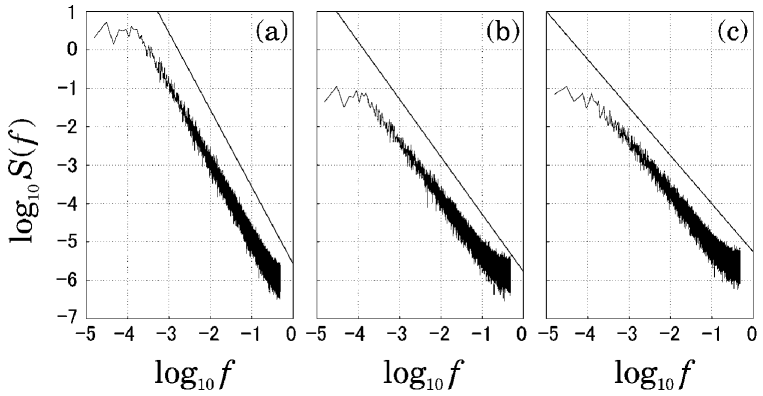
Figure 5: PSD of the signal in each step in the procedure to achieve a $1/f$ noise. PSD is obtained by averaging over $10$ samples. The straight lines represent $f^{-2}$ in (a), $f^{-1.5}$ in (b) and $f^{-1.25}$ in (c). (a) PSD of a Lorentzian noise. (b) PSD of the noise transformed once. (c) PSD of the noise transformed twice. To obtain a Gaussian input noise, five output noises by the previous transformation were averaged.

There are several methods to generate $1/f^{\alpha}$ noise[3, 12, 13, 14] ; among them, McWhoter’s model for $1/f$ noise is well known because the model corresponds to real physical systems, for example, noise due to surface traps of carriers in a semiconductor.[12] McWhoter’s theory tells that if a large number of Lorentzian noises with various relaxation time $\tau$ are superposed with an appropriate weight: $w(\tau)\propto 1/\tau$ in a range $\tau_{2}\leq\tau\leq\tau_{1}$, the spectrum becomes $1/f$ in the frequency range $1/\tau_{1}\ll f\ll 1/\tau_{2}$. In contrast to McWhoter’s theory, the present method requires only one kinds of Lorentzian noises specified by a single relaxation time $\tau_{1}$: $w(\tau)=\delta(\tau-\tau_{1})$. Then the dichotomous transformation, if applied repeatedly, can lead to nearly $1/f$ noise in the range $f\gg 1/\tau_{1}$.

In many cases, model systems exhibit $1/f$ noise only when the system parameters are tuned to some special values. For example, simulations of phonon number fluctuations based on a Fermi-Pasta-Ulam lattice resulted in a $1/f$ spectrum when the lattice size is $N=8$.[15, 16] For larger $N$, however, the spectrum tended to Lorentzian $\sim(f^{2}+f_{0}^{2})^{-1}$, although the time scale $\tau_{1}\equiv 1/f_{0}$ became larger as $N$ increases.[16] In contrast, tuning is unnecessary in the present method of generating $1/f$ noise, which is an essential point of the method.

§6 Summary and Discussions

We have analyzed the amplitude truncation of $1/f^{\alpha}$ noises (eq. (1.1)). Although $1/f^{\alpha}$ noises with $\alpha$ between $0$ and $2$ are commonly called ‘$1/f$ noise’, the transformation property is different depending on whether $\alpha$ is larger than unity or not.

For $\alpha>1$, the output PSD under the symmetrical truncation obeys the power law with a smaller exponent $\beta=(\alpha+1)/2$ (which is still larger than unity) in a low frequency range ($f_{1}\ll$)$f\ll f_{\rm c}$. The corner frequency $f_{\rm c}$ depends on $\alpha$ and the truncation level $a$ as $f_{\rm c}\propto a^{-2/(\alpha-1)}$. Let us assume that the time scale of the system, $\tau_{1}=1/f_{1}$, is long enough so that the interval $[f_{1}$, $f_{\rm c}]$ is sufficiently wide. Then the filtering effect in the measurement makes it possible to observe a power law spectrum with the exponent much smaller than $2$, even if the original signal is close to Lorentzian: $\alpha\sim 2$. As was shown by the numerical simulation, if we start from an ensemble of Gaussian $1/f^{2}$ or Lorentzian signals and apply the symmetrical truncation and re-Gaussianization procedure repeatedly, the output signal converges to $1/f$ noise.

When $\alpha\leq 1$, in contrast, the symmetrical truncation leads to a power law spectrum with the same exponent $\alpha$. (A proof for $\alpha=1$ has been given only for the dichotomous transformation.[1]) This means that the exponent less than unity can never be reached by the symmetrical truncation as far as we start from the exponent larger than unity. On the other hand, when the asymmetrical amplitude truncation is applied to $1/f^{\alpha}$ signal with $\alpha$ less than unity, the output PSD deviates from the power law. The correction terms make the slope of the spectrum flatter as $f$ increases. However, as far as the results of the numerical experiments ($\alpha=0.8$ in the present paper and $\alpha=1$ in ref. 5) are observed, the output PSD looks approximately as $1/f^{\alpha}$-like with an exponent smaller than that of the input signal.

Amplitude truncation may generally occurs in systems composed of threshold elements, for example neural networks. It also occurs in the flow of packets in Internet systems where the overflow of the packets is deleted. Furthermore, measurement or analysis of signals often involves amplitude truncation. For example, a dichotomous transformation is used to analyze the (spatial) long-range correlation in DNA.[10] If a Lorentzian or $1/f^{2}$ noise is superposed on the original signal, filtering with such a truncation may easily leads to the observation of a $1/f^{\alpha}$ noise.

Throughout the present paper, we have assumed that the time scale of the system is long enough so that the original data exhibits the power law spectrum in a wide range of frequencies. As mentioned already, to derive an extremely long time scale from any realistic model is a difficult problem. Once a long time scale has been assumed, however, the present study suggests a possible mechanism to generate $1/f^{\alpha}$ noises with the exponent smaller than that of the original signal.

References

[1]
S. Ishioka, Z. Gingl, D. Choi and N. Fuchikami:
Phys. Lett. A 269 (2000) 7.
[2]
P.Bak: How Nature Works (Oxford University Press, New York, 1997).
[3]
B. R. Frieden and R. J. Hughes:
Phys. Rev. E 49 (1994) 2644.
[4]
B. B. Mandelbrot and J. R. Wallis:
Water. Resour. Res. 5 (1969) 321.
[5]
T. Musha, G. Borbery and M. Shoji:
Phys. Rev. Lett. 64 (1990) 2394.
[6]
N. Fuchikami:
Phys. Rev. E 60 (1999) 1060.
[7]
Z. Gingl and L.B. Kiss: Proc. First Int. Conf. on Unsolved
Problems of Noise edited by Ch.R. Doering, L.B. Kiss and
M.F. Schlesinger (World Scientific, 1996) p.337.
[8]
Z. Gingl, S. Ishioka, D. Choi and N. Fuchikami:
Proc. Int. Conf. on Unsolved
Problems of Noise and Fluctuation edited by D. Abbott and L.B. Kish
(AIP. press, 1999) p.136.
[9]
Note that the output signal is generally non-Gaussian.
[10]
H.E.Stanly, S.V.Buldyrev, A.L.Goldberger, Z.D.Goldberger,
S.Hvlin, R.N.Mantegna, S.M.Oddadnik, C.-K.Peng and M.Dimons:
Physica A 205 (1994) 214.