Passive scalar intermittency in low temperature helium flows

Abstract

We report new measurements of turbulent mixing of temperature fluctuations in a low temperature helium gas experiment, spanning a range of microscale Reynolds number, $R_{\lambda}$, from 100 to 650. The exponents $\xi_{n}$ of the temperature structure functions $\langle|\theta(x+r)-\theta(x)|^{n}\rangle\sim r^{\xi_{n}}$ are shown to saturate to $\xi_{\infty}\simeq 1.45\pm 0.1$ for the highest orders, $n\sim 10$. This saturation is a signature of statistics dominated by front-like structures, the cliffs. Statistics of the cliff characteristics are performed, particularly their width are shown to scale as the Kolmogorov length scale.

The strong intermittency of a passive scalar field advected by a turbulent flow has recently received considerable attention [1, 2]. Two facets of this intermittency are the persistence of small scale anisotropy [3, 4] and the anomalous scaling of the structure functions $\langle|\theta(x+r)-\theta(x)|^{n}\rangle$ [5, 6]. It is well established that the persistence of scalar gradient skewness arises from the ramp-and-cliff structures [3, 4], i.e high scalar jumps separated by well mixed regions. The observed preferential alignment of cliffs with the large scale gradient [7, 8] apparently prevents a universal description of the odd order statistics, reflecting the asymetry of scalar fluctuations. However, the genericity of cliffs in “scalar turbulence” raises the issue of their influence on high-order scaling of even moments, and of the possible universality of the suspected saturation of high order exponents [9, 10, 11]. Laboratory experiments able to cover a wide range of Reynolds numbers in well controlled conditions appear to be crucial to address this point. We report in this Letter new measurements of turbulent mixing of a scalar field, namely temperature fluctuations, performed in a low temperature helium gas experiment. Such measurements of temperature fluctuations, as a passively advected scalar field, are performed for the first time in low temperature helium gas [12], opening new and encouraging perspectives in investigation of turbulent mixing in high Reynolds number flows.

The set-up we use is the same as the one described in Ref. [13], with an additional apparatus to induce temperature fluctuations. The flow takes place in a cylindrical vessel and is driven by two rotating disks, as sketched in Fig. 1. The disks, 20 cm in diameter and spaced 13.1 cm apart, are mounted with 6 radial blades. The cell is filled with helium gas, held at a controlled pressure. Temperature measurements are performed with a specially designed cold-wire thermometer in the thermal wake of a heated grid. The grid is made of a double nichrome wire net, stretched across a $4.0\times 4.5$ cm frame. The wire diameter is 250 $\mu$m, and the mesh size, $M$, is 2.0 mm.

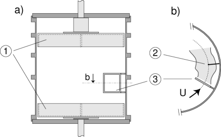
FIG. 1.: (a) Sketch of the experiment. (b) Upper view, in corotating mode. (1) Disks, (2) thermometer, (3) heated grid.

The thermometer is located 20 mesh sizes downstream from the grid, at a distance of 2.2 cm from the wall. It has been designed as the velocity probes described in Ref. [13]. It consists in a thin carbon fiber, 7 $\mu$m in diameter, stretched across a 2 mm rigid frame. A metallic deposition of gold and silver of about 2000 Å thick covers the whole fiber, except for a 7 $\mu$m long central area. Temperature fluctuations are measured from resistance fluctuations, by the way of a constant current Wheatstone bridge. The tuning of the current has received considerable attention, in order to ensure an high enough signal, without suffering from velocity contamination. In practice, the optimal value of the current is chosen in order to maximize the flatness factor of the temperature derivative. Temperature resolution is estimated, from the high-frequency white noise level, to around 100 $\mu$K. The spatial resolution is limited by the probe size, which is at least twice smaller than the Kolmogorov scale in the present experiments. The frequency response is limited by the constant current amplifier to 10 kHz, a value comfortably high to resolve the highest frequency of the temperature fluctuations.

Since the same probe, with different electronic devices, is used as both thermometer and anemometer, we are able to perform temperature and velocity measurements at the same point in the same flow conditions. We have measured the various turbulence characteristics, such as the microscale Reynolds number $R_{\lambda}$ and the Kolmogorov scale $\eta$, for the same disks rotation rates and kinematic viscosity $\nu$, allowing us to characterize each temperature data set. We define here $R_{\lambda}=u^{\prime}\lambda/\nu$ the Reynolds number based on the Taylor scale $\lambda=u^{\prime}(\nu/\epsilon)^{1/2}$, where $u^{\prime}$ is the rms of the velocity fluctuations, $\epsilon$ the mean dissipation rate and $\eta=(\nu^{3}/\epsilon)^{1/4}$.

The disks rotation can be set in two modes, co- and counter-rotating, hereafter denoted by COR and CTR. In the corotating mode, the two disks are rotating in the same direction at the same speed, so that the flow can be thought as a solid-like rotation. The fluctuation rate $u^{\prime}/\langle U\rangle$ is found to lie around 10 % in this case, a value close to the one obtained in a previous experiment in a similar set-up [14]. In the counter-rotating mode, the turbulence intensity is much higher, but the speed ratio is tuned so that a strong mean advection remains at the height of the grid and the thermometer. This ensures a low enough fluctuation rate, between 13 and 25 %, allowing use of the Taylor hypothesis to convert temporal fluctuations into spatial ones. We have checked that the fluctuation rate is the same with and without the grid, meaning that the grid contribution to the turbulence can be considered as negligible. The only influence of the grid is injection of heated sheets in an already turbulent flow. Thus thermal turbulence originates in the mixing of these hot layers behind each wire, over a typical distance of $M\langle U\rangle/u^{\prime}=$1–2 cm downstream.

The grid temperature has to be high enough to induce thermal fluctuations giving rise to an acceptable signal to noise ratio of at least 50 dB. The noise level of 100 $\mu$K requires a rms signal of typically $\theta^{\prime}=\langle\theta^{2}\rangle^{1/2}\simeq 40$ mK at the probe location, which is around 4 % of the grid overheat. Since we are working with a closed flow, the heat transfer from the cell to the cryostat has to be balanced by the power supplied to the grid, in order to ensure thermal stationarity. This constraint limits the maximum duration of an experiment (up to 5 hours of continuous run), and the range of velocity and fluid density; in practice, values of $R_{\lambda}$ in the range 100–300 in the corotating case, and 200–650 in the counter-rotating case, are obtained. Although much lower than the highest $R_{\lambda}$ achievable in our set-up (up to 5000 [13]), we hope that future noise improvement of the constant current amplifier will increase the upper bound well beyond 650.

File no.	$10^{4}\times\kappa$	$R_{\lambda}$	$\langle U\rangle$	$\theta^{\prime}$	$10^{-6}\,N^{*}$
	(cm2/s)		(cm/s)	(mK)
1 COR	75	105	16.3	45.5	0.84
2 COR	17	280	27.4	56.8	14.7
3 CTR	17	360	28.2	96.0	30.6
4 CTR	17	650	34.4	69.0	85.7

TABLE I.: Typical experimental parameters. $\kappa=\nu/\mbox{Pr}$ is the thermal diffusivity, $\nu$ the kinematic viscosity and $\mbox{Pr}\simeq 0.8$. The sample size $N^{*}$ is expressed as $N\langle U\rangle/(2\pi f_{s}\eta)$, where $N$ is the number of data points of the sample and $f_{s}$ the sampling rate.

The temperature signal is filtered, then sampled and recorded on a 16 bit acquisition board (ITC-18 from InstruTech), at a sampling rate between 1 and 10 kHz, a value at least twice the low-pass filter frequency. Special attention has been paid to the low noise level of the whole amplifying and sampling channel. In order to achieve correct convergence of higher-order statistics, the sample sizes are of the order of $10^{7}-10^{8}$ Kolmogorov time scales long. Table I summarizes the characteristics of the typical data sets used here.

In order to characterize the large scale of the temperature and velocity fluctuations, quantities of interest are the integral scales $\Lambda_{\theta}$ and $\Lambda_{u}$, defined from the autocorrelation functions of temperature $\theta$ and longitudinal velocity $u$. For our whole data set, we measure $\Lambda_{\theta}=7.0\pm 1.5$ mm and $\Lambda_{u}=9.6\pm 1.0$ mm, with no noticeable $R_{\lambda}$ dependence [14]. This two values are rather close, indicating that kinetic energy and temperature variance are injected at the same large scale. The Prandtl number of the gas being close to unity, we are on the case where velocity and scalar fluctuations take place on the same range of scales.

FIG. 2.: Probability density functions of the normalized temperature increments, for $R_{\lambda}=650$ (file #4 of Tab. I). From the inner to the outer pdf, $r/\eta=10^{4}$, 600, 30 and 3.

The small scale intermittency of temperature fluctuations can be characterized through their distributions at different scales. Figure 2 shows the probability density functions (pdf) of temperature increments $\Delta\theta(r)=\theta(x+r)-\theta(x)$ for 4 different separations $r$, ranging from $r/\eta$ = 10⁴ (large scale), 600, 30 (typical inertial scales) down to 3 (close to the dissipative scale). Each distribution has been normalized by its standard deviation $\sigma=\langle\Delta\theta(r)^{2}\rangle^{1/2}$. These pdf are strongly not self-similar, reflecting strong intermittency effects. The width of the tails is remarkable, showing scalar jumps of amplitude up to 40 times the standard deviation at the smallest scale. We can note the slight asymmetry of the distributions, linked to the well known property of small scale persistence of anisotropy [2].

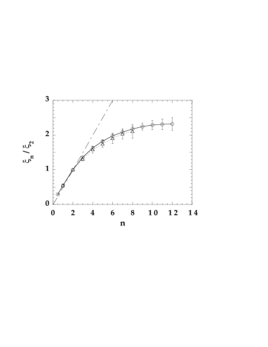
FIG. 3.: Temperature structure function exponents, $\xi_{n}$, normalized by $\xi_{2}$. $\bigcirc$: $R_{\lambda}=280$ in COR mode, $\triangle$: $R_{\lambda}=650$ in CTR mode. The dashed line indicates the Corrsin-Obukhov scaling $n/2$.

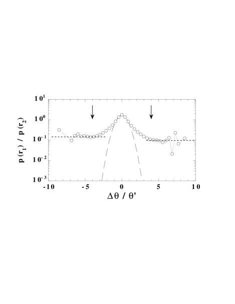
FIG. 4.: Ratio of two pdfs, at different inertial scales, $r_{1}=45\eta$ and $r_{2}=246\eta$ ($R_{\lambda}=280$). The long dashed curve is a gaussian fit, and the horizontal dashed lines indicate the constant ratio of the pdf tails. Vertical arrows, at $\Delta\theta\simeq 4\theta^{\prime}$, indicate the dominant contribution to the 8th order moment.

The evolution of these pdfs is characterized by the structure functions, defined as $S_{n}(r)=\langle|\theta(x+r)-\theta(x)|^{n}\rangle$, where angular brackets denote space (time) average. They are found to follow power law in terms of the scale $r$, namely $S_{n}(r)\sim r^{\xi_{n}}$. The measured structure function exponents $\xi_{n}$, divided by $\xi_{2}$, are shown in Fig. 3, in the COR ($R_{\lambda}=280$) and CTR ($R_{\lambda}=650$) cases. The exponents are defined by plotting the compensated structure functions $r^{-\xi_{n}}S_{n}(r)$ and tuning the value of the exponent to obtain a well defined plateau for inertial separations. This procedure allows to estimate the error bar for each order. Although the second order exponent presents some scatter (with a systematic increase from 0.45 to 0.65 with increasing $R_{\lambda}$), the normalization of the higher order exponents by $\xi_{2}$ provides an excellent collapse for the different $R_{\lambda}$. It is remarkable that, for comparable sample sizes, the highest available order is much lower at higher Reynolds number: the fluctuations becomes much more intermittent and the convergence becomes poorer. For $R_{\lambda}=650$ we have to restrict to $n\leq 8$, whereas $n=12$ can be achieved for $R_{\lambda}=280$. The two sets of exponents are consistent within error bars for $n\leq 8$, meaning that the large scale properties of the two flow configurations do not affect these inertial range statistics.

The values of $\xi_{n}/\xi_{2}$ are found to strongly depart from the linear law $n/2$, and the gap increases with the order, a usual signature of inertial range intermittency of the passive scalar[2]. Furthermore, the exponents are found to increase extremely slowly with the order, strongly suggesting a saturation, for $n$ around 10, at a value

$$\xi_{\infty}=(2.3\pm 0.1)\xi_{2}\simeq 1.45\pm 0.1$$ (1)

(where $\xi_{2}$ is considered equal to 2/3). This observation only relies on the COR data set, but we have noted that no deviation appears between the COR and CTR data for $n\leq 8$. A saturation of the structure function exponents is a signature of statistics dominated by shock-like structures, the thermal cliffs. A consequence of this saturation is a constant ratio of the far tails of the pdfs for inertial range separations. The ratio of two pdfs, for separations $r_{1}$ and $r_{2}$ well into the inertial range, is displayed in Fig. 4. For temperature increments $|\Delta\theta|>4\theta^{\prime}$, this ratio tends towards a constant. It must be noted that the $|\Delta\theta|\simeq 4\theta^{\prime}$ parts of this distribution give the dominant contribution to the 8th order moment (see the vertical arrows), i.e they maximize the integrant $|\Delta\theta|^{8}p(\Delta\theta)$. This additional test confirms the observed saturation of high order exponents.

FIG. 5.: Histograms of cliff width (a) and amplitude (b) for values of the threshold $s=3$ ($\bigcirc$), 7 ($\Box$) and 11 ($\diamond$). The dashed curves on the figure (b) are log-normal fits.

The observed trend towards a saturation of high order exponents motivates a detailed analysis of the cliffs. We have performed statistics of the cliff characteristics, defined as the strongest temperature gradients, singled out from time series of temperature fluctuations. We define the cliffs from a simple threshold on the temperature derivative,

$$|\partial\theta/\partial x|>s\,\langle(\partial\theta/\partial x)^{2}\rangle^{1/2},$$ (2)

where $s$ is a non dimensional constant. Spatial derivatives are obtained from temporal ones using the Taylor hypothesis, and the gradients are estimated from finite difference over the smallest resolved separation. We define the cliff amplitude $\delta\theta$ as the difference between the two extrema surrounding the gradient satisfying (2), and the cliff width $\Delta$ such that the temperature derivative takes values exceeding 90 % of its local maximum. Histograms of amplitudes and widths are shown in Fig. 5, for three values of the threshold $s$, at a Reynolds number $R_{\lambda}=280$.

We first note that both amplitude and width histograms can be well fitted by log-normal distributions (given by a parabola in log-log coordinates). The mean amplitude of the cliffs is of order $\theta^{\prime}$, and is found to increase with the threshold $s$. On the other hand, the cliff width remains constant for different thresholds. This means that the strength of the gradients depends mainly on the amplitude of the scalar jump, and not on its width.

FIG. 6.: Mean cliff width divided by the Kolmogorov length scale, as a function of $R_{\lambda}$. $\bigcirc$: COR, $\triangle$: CTR. The dashed line is the average, $\langle\Delta\rangle/\eta\simeq 13$.

A central issue concerning the cliffs is the Reynolds number dependence of their width. Figure 6 shows the mean cliff width $\langle\Delta\rangle$, divided by the Kolmogorov scale $\eta$, for $R_{\lambda}$ ranging from 100 to 650. This plot extends a preliminary study [16] performed only on the COR mode. We can see a well defined plateau,

$$\langle\Delta\rangle=(13\pm 3)\eta.$$ (3)

The scatter is moderate, and probably reflects the difficulty to resolve properly the smallest scales. However, this plot confirms that the mean cliff width follows a $R_{\lambda}^{-3/2}$ scaling. This law holds for values of the threshold $s$ from 3 up to 40 in the case of the highest $R_{\lambda}$ (see Fig. 2). We can note that the data from the two configurations overlap on the central region $R_{\lambda}=200-300$, suggesting that this small scale characteristics is not affected by the large scale properties of the flow.

To summarize, we have performed for the first time measurements of turbulent mixing of temperature, considered as a passive scalar field, in a low temperature helium experiment. The study of inertial range statistics of the temperature increments gives evidence of a saturation of the high order exponents, to a value $\xi_{\infty}\simeq 1.45\pm 0.1$. This observation reveals that inertial range statistics are dominated by the cliffs, concentrating large scalar jumps over small distance [9, 10, 11]. The cliff widths are shown to scale as the Kolmogorov length scale, in the whole range of observed $R_{\lambda}$ (100–650), suggesting that the strongest cliffs remain concentrated over the smallest scale of the flow (see also Ref. [15]). This observation may have important consequences for processes such as reactive mixing or combustion, where the reaction rate is enhanced where concentration gradients are strong. Further insight into the cliffs contribution to the saturation of the high order structure function exponents needs a detailed study of their morphology and spatial distribution. Preliminary results [16], based on the waiting time between cliffs from the temperature time series, strongly suggests self-similar clustering for inertial separations.

The authors thank B. Shraiman, V. Hakim, M. Vergassola, P. Castiglione and M.C. Jullien for fruitful discussions. This work has been supported by Ecole Normale Supérieure, CNRS, the Universities Paris 6 and Paris 7, and the European Commission’s TMR programme, Contract no. ERBFMRXCT980175 “Intermittency”.

REFERENCES

- [1] B.I. Shraiman and E. Siggia, Nature 405, 639 (2000).
- [2] Z. Warhaft, Annu. Rev. Fluid. Mech. 32, 203 (2000).
- [3] P.G. Mestayer, C.H. Gibson, F.M. Coantic, and A.S. Patel, Phys. Fluid. 19 (9), 1279 (1976).
- [4] C.H. Gibson, C.A. Friehe and S.O. McConnell, Phys. Fluid. 20, S156 (1977).
- [5] R.A. Antonia, E. Hopfinger, Y. Gagne and F. Anselmet, Phys. Rev. A 30, 2704 (1984).
- [6] R.H. Kraichnan, Phys. Rev. Lett. 72 (7), 1016 (1994).
- [7] M. Holzer and E. Siggia, Phys. Fluid 6 (5), 1820 (1994).
- [8] A. Pumir, Phys. Fluid. 6 (6), 2118 (1994). Phys. Fluid. 6 (12), 3974 (1994).
- [9] V. Yakhot, Phys. Rev. E 55,329 (1997).
- [10] A. Celani, A. Lanotte, A. Mazzino and M. Vergassola, Phys. Rev. Lett. 84, 2385 (2000)
- [11] M.C. Jullien, P. Castiglione and P. Tabeling, subm. to Phys. Rev. Lett.
- [12] Flow at ultra-high Reynolds and Rayleigh numbers, a status report, edited by R.J. Donnelly and K.R. Sreenivasan (Springer-Verlag, New York, 1998).
- [13] G. Zocchi, P. Tabeling, J. Maurer and H. Willaime, Phys. Rev. E 50 (5), 3693 (1994). F. Moisy, P. Tabeling and H. Willaime, Phys. Rev. Lett. 82, 3994 (1999).
- [14] H. Willaime, J. Maurer, F. Moisy and P. Tabeling, to appear in Eur. Phys. J. B (2000).
- [15] F.T.M. Nieuwstadt and G. Brethouwer, Advances in Turbulence VIII, edited by C. Dopazo (CIMNE, Barcelona, 2000), 133.
- [16] F. Moisy, H. Willaime, J.S. Andersen and P. Tabeling, Advances in Turbulence VIII, edited by C. Dopazo (CIMNE, Barcelona, 2000), 835.