To be published in Comp. Phys. Commun.  Force calculation and atomic-structure optimization for the full-potential linearized augmented plane-wave code WIEN

Abstract

Following the approach of Yu, Singh, and Krakauer [Phys. Rev. B 43 (1991) 6411] we extended the linearized augmented plane wave code WIEN of Blaha, Schwarz, and coworkers by the evaluation of forces. In this paper we describe the approach, demonstrate the high accuracy of the force calculation, and use them for an efficient geometry optimization of poly-atomic systems.

PROGRAM SUMMARY

Title of program extension: fhi95force
catalogue number: …
Program obtainable from: CPC Program Library, Queen’s University of Belfast, N. Ireland (see application form in this issue)
CPC Program Library programs used: cat. no.: ABRE; title: WIEN; ref. in CPC: 59 (1990) 399
Licensing provisions: none
Computer, operating system, and installation:

• IBM RS/6000; AIX; Fritz-Haber-Institut der Max-Planck-Gesellschaft; Berlin.

• CRAY Y-MP; UNICOS; IPP der Max-Planck-Gesellschaft; Garching.

Operating system: UNIX
Programming language: FORTRAN77
(non-standard feature is the use of ENDDO)
floating point arithmetic: 64 bits
Memory required to execute with typical data:
64 Mbyte (depends on case)
No. of bits in a word: 64
No. of processors used: one
Has the code been vectorized? no
Memory required for test run:  64 MByte
Keywords
density functional theory, linearized augmented plane wave method, LAPW, supercell, total energy, forces, structure optimization, molecular dynamics, crystals, surfaces, molecules
Nature of the physical problem
For ab-initio studies of the electronic and magnetic properties of poly-atomic systems, such as molecules, crystals, and surfaces, it is of paramount importance to determine stable and metastable atomic geometries. This task of structure optimization is greatly accelerated and, in fact, often only feasible if the forces acting on the atoms are known.
The computer-code described in this article enables such calculations.
Method of solution
The full-potential linearized augmented plane wave (FP-LAPW) method is well known to enable accurate calculations of the electronic structure and magnetic properties of crystals [1, 2, 3, 4, 5, 6, 7, 8]. Within the supercell approach it has also been used for studies of defects in the bulk and for crystal surfaces. For the evaluation of the atomic forces within this method we follow the approach outlined by Yu and coworkers [9]. In order to minimize the total energy as a function of atomic positions we employ a damped Newton dynamics scheme [10] or alternatively the variable metric algorithm of Broyden et al. [11, 12, 13]. Several applications of this approach to chemisorption at surfaces have already been published [14, 15].
Restrictions on the complexity of the problem
Inversion and orthorombic symmetry of the elementary cell is required.
Typical running time
The additional force calculation increases the running time of a typical self-consistent total energy calculation by 5-10%.
References

LONG WRITE-UP

1 Introduction

The augmented plane wave (APW) methods [1, 2, 3, 4, 5] and in particular its linearized form, the LAPW [6, 7, 8, 9, 10, 11, 12, 13, 14], enable accurate calculations of the electronic and magnetic properties of poly-atomic systems from first principles. One successful implementation is the program package WIEN. This full-potential LAPW (FP-LAPW) code developed by Blaha, Schwarz and coworkers [13] has been successfully applied to a wide range of problems [15, 16] and systems such as complex crystals [17], transition metal surfaces [18], and molecules (see the H₂ test case in this paper).

The main output of the WIEN code is the total energy for a given atomic arrangement. Using only this quantity the minimization of the total energy of a poly-atomic system is a costly and often impractible task. However, the situation is changed if the forces which act on the different atoms are available. Only recently, force formulations within the LAPW method have been introduced and tested by several authors [19, 20, 21, 22, 23, 24]. We followed the approach of Yu, Singh, and Krakauer (YSK) [20] and implemented the direct calculation of atomic forces into the original [13] and the WIEN93 version [25] of the WIEN code. The obtained forces are highly accurate and can be used in an efficient minimization scheme to optimize the geometry of poly-atomic systems.

The remainder of the paper is organized as follows. In Sec. II we summarize the most important features of the YSK force formalism. Section III describes the energy minimization procedure. In Sec. IV results of test calculations are presented, and, finally, Sec. V and VI describe the structure and the installation of our program package fhi95force.

2 Evaluation of Forces

2.1 Forces within Density-Functional Theory

Within density-functional theory the ground state total energy is given by the minimum of a total energy functional with respect to the electron density $n(\vec{r})$

$$E^{\rm tot}[n]=T[n]+U[n]+E^{\rm xc}[n]$$ (1)

where $T[n]$, $U[n]$, and $E^{\rm xc}[n]$ represent the functionals of the non-interacting many electron kinetic, the electrostatic, and the exchange-correlation (xc) energy, respectively. The electron density $n^{\rm sc}(\vec{r})$ which minimizes $E^{\rm tot}[n]$ is found by solving self-consistently the Kohn-Sham (KS) equations [26, 27]

$$H\psi_{i}(\vec{r})=[\hat{T}+V^{\rm eff}(\vec{r})]\psi_{i}(\vec{r})=\epsilon_{i}\psi_{i}(\vec{r})$$ (2)

where $\hat{T}$ is the single-particle kinetic energy operator. Throughout the paper we use Rydberg atomic units. The effective potential $V^{\rm eff}(\vec{r})$ is given by

$$V^{\rm eff}(\vec{r})=V^{\rm es}(\vec{r})+V^{\rm xc}(\vec{r})$$ (3)

where

$$V^{\rm es}(\vec{r})=\int d^{3}\vec{r}\,^{\prime}\,\frac{n(\vec{r}\,^{\prime})}{|\vec{r}-\vec{r}\,^{\prime}|}-\sum_{I}\frac{Z_{I}}{|\vec{r}-\vec{R}_{I}|}$$ (4)

denotes the total electrostatic potential created by the electron density

$$n(\vec{r})=\sum_{i=1}^{\infty}f_{i}\psi_{i}^{*}(\vec{r})\psi_{i}(\vec{r})$$ (5)

and the nuclear charges. The quantities $f_{i}$ are the occupation numbers of the eigenstates $\psi_{i}(\vec{r})$. The $I$-th nucleus is positioned at $\vec{R}_{I}$ and carries the charge $Z_{I}$. The xc potential $V^{\rm xc}(\vec{r})$ is

$$V^{\rm xc}(\vec{r})=\frac{\delta E^{\rm xc}[n]}{\delta n}\quad.$$ (6)

The KS total energy $E^{\rm tot}[n]$ is then calculated by using the expressions

$$T[n] = \sum_{i=1}^{\infty}f_{i}\epsilon_{i}-\int d^{3}\vec{r}\,n(\vec{r})V^{\rm eff}(\vec{r})$$

$$U[n] = \frac{1}{2}\int d^{3}\vec{r}\,d^{3}\vec{r}\,^{\prime}\,\frac{n(\vec{r})n(\vec{r}\,^{\prime})}{|\vec{r}-\vec{r}\,^{\prime}|}-\int d^{3}\vec{r}\,n(\vec{r})\sum_{I}\frac{Z_{I}}{|\vec{r}-\vec{R}_{I}|}+\frac{1}{2}\sum_{I\neq J}\frac{Z_{I}Z_{J}}{|\vec{R}_{I}-\vec{R}_{J}|}$$

$$E^{\rm xc}[n] = \int d^{3}\vec{r}\,n(\vec{r})\epsilon^{\rm xc}\left[n\right](\vec{r})\quad,$$ (7)

where $\epsilon^{\rm xc}[n]$ is the xc energy per particle. For finite temperatures, or in order to stabilize the convergence of the self-consistent calculation the electronic states may be occupied according to a Fermi distribution at a non-zero electron temperature $T^{\rm el}$

$$f_{i}=\left[1+\exp\left(\frac{\epsilon_{i}-\epsilon_{\rm F}}{k_{\rm B}T^{\rm el}}\right)\right]^{-1}$$ (8)

where $\epsilon_{\rm F}$ and $k_{\rm B}$ are the Fermi energy and the Boltzmann constant. In this case, one has to minimize the free energy [28, 29]

$${\cal F}[n]=E^{\rm tot}[n]-T^{\rm el}S^{\rm el}$$ (9)

with the entropy $S^{\rm el}$ given by

$$S^{\rm el}=-2k_{\rm B}\sum_{i}\left[f_{i}\log f_{i}+(1-f_{i})\log(1-f_{i})\right]-S_{0}\quad.$$ (10)

Here, $S_{0}$ is chosen such that the entropy $S^{\rm el}$ vanishes for $T^{\rm el}=0$ K. The force on the $I$-th nucleus is defined as the negative derivative of the free energy with respect to the nuclear coordinate $\vec{R}_{I}$:

$$\vec{F}_{I}=-\left.\frac{dE^{\rm tot}-T^{\rm el}dS^{\rm el}}{d\vec{R}_{I}}\right|_{n(\vec{r})=n^{\rm sc}(\vec{r})}\quad.$$ (11)

It is evaluated by displacing the respective nucleus by a small amount $\Delta\vec{R}_{I}$ and calculating the resulting first-order change of the free energy $\Delta{\cal F}$. For the different energy terms in eq. (7) we obtain the following first order variations

$$\Delta T[n] = \sum_{i=1}^{\infty}\Delta f_{i}\epsilon_{i}+\sum_{i=1}^{\infty}f_{i}\Delta\epsilon_{i}-\int d^{3}\vec{r}\,\Delta n(\vec{r})V^{\rm eff}(\vec{r})-\int d^{3}\vec{r}\,n(\vec{r})\Delta V^{\rm eff}(\vec{r})$$

$$\Delta U[n] = \int d^{3}\vec{r}\,\Delta n(\vec{r})V^{\rm es}(\vec{r})-\vec{F}_{I}^{\rm HF}\Delta\vec{R}_{I}$$

$$\Delta E^{\rm xc}[n] = \int d^{3}\vec{r}\,\Delta n(\vec{r})V^{\rm xc}(\vec{r})\quad.$$ (12)

The first term $\sum_{i}\Delta f_{i}\epsilon_{i}$ in $\Delta T[n]$ is canceled with the contribution from the variation of the entropy $S^{\rm el}$ in eq. (11) [30]. The Hellmann-Feynman (HF) force $\vec{F}_{I}^{\rm HF}$ describes the classical electrostatic force exerted on the $I$-th nucleus by all the other charges of the system (electrons and nuclei) [31, 32] and is obtained from

$${\vec{F}}_{I}^{\rm HF}=Z_{I}\nabla_{\vec{r}}V_{I}^{\rm es}(\vec{r})|_{\vec{r}=\vec{R}_{I}}$$ (13)

where $V_{I}^{\rm es}(\vec{r})$ is the electrostatic potential

$$V_{I}^{\rm es}(\vec{r})=V^{\rm es}(\vec{r})+\frac{Z_{I}}{|\vec{r}-\vec{R}_{I}|}$$ (14)

felt by the $I$-th nucleus. Taking the definition of the effective potential in eq. (3) into account the force on the $I$-th nucleus is then given by

$$\vec{F}_{I}=\vec{F}_{I}^{\rm HF}-\frac{1}{\Delta\vec{R}_{I}}\left\{\sum_{i=1}^{\infty}f_{i}\Delta\epsilon_{i}-\int d^{3}\vec{r}\,n^{\rm sc}(\vec{r})\Delta V^{\rm eff}(\vec{r})\right\}\quad.$$ (15)

It should be mentioned that the free energy variation $\Delta{\cal F}$ and thus the forces $\vec{F}_{I}$ are invariant to any first order deviation $\Delta n(\vec{r})$ from the self-consistent density $n^{\rm sc}(\vec{r})$. Thus, force expressions different from eq. (15) may be derived if this variational freedom is used, e.g. if the electron density is shifted rigidly with the nuclei [33, 34, 35].

2.2 Basis Set Corrections to the Hellmann-Feynman Force

Usually, the HF force $\vec{F}_{I}^{\rm HF}$ can be evaluated quite easily using eq. (13). The second term in eq. (15) describes the so-called Pulay forces [36]. The explicit expression of this correction to the HF force $\vec{F}_{I}^{\rm HF}$ depends on how the KS equation is solved. One usually expands a KS wavefunction $\psi\equiv\psi_{i}(\vec{r})$ at the eigenvalue $\epsilon\equiv\epsilon_{i}$ linearly using a set of basis functions $\phi_{\nu}$:

$$\psi=\sum_{\nu}C_{\nu}\phi_{\nu}\quad.$$ (16)

With this variational basis functions, the KS equation becomes the following secular equation

$$\sum_{\mu}\left(H_{\mu\nu}-\epsilon O_{\mu\nu}\right)C_{\nu}=0\quad,$$ (17)

or equivalently

$$\sum_{\mu\nu}C^{*}_{\mu}\left(H_{\mu\nu}-\epsilon O_{\mu\nu}\right)C_{\nu}=0\quad.$$ (18)

The Hamilton and overlap matrix elements are defined as

$$H_{\mu\nu} = \langle\phi_{\mu}|H|\phi_{\nu}\rangle$$ (19)

$$O_{\mu\nu} = \langle\phi_{\mu}|\phi_{\nu}\rangle\quad.$$ (20)

Both eqs. (17) and (18) also hold for a shifted atomic configuration ${\vec{R}_{I}+\Delta\vec{R}_{I}}$. Thus, we obtain for the latter

$$\sum_{\mu\nu}\left(C^{*}_{\mu}+\Delta C^{*}_{\mu}\right)\left[H_{\mu\nu}+\Delta H_{\mu\nu}-(\epsilon+\Delta\epsilon)(O_{\mu\nu}+\Delta O_{\mu\nu})\right]\left(C_{\nu}+\Delta C_{\nu}\right)=0\quad.$$ (21)

The variations of the matrix elements are as follows:

$$\Delta O_{\mu\nu} = \langle\Delta\phi_{\mu}|\phi_{\nu}\rangle+\langle\phi_{\mu}|\Delta\phi_{\nu}\rangle=2\mbox{Re}\langle\Delta\phi_{\mu}|\phi_{\nu}\rangle$$ (22)

$$\Delta H_{\mu\nu} = 2\mbox{Re}\langle\Delta\phi_{\mu}|H|\phi_{\nu}\rangle+\langle\phi_{\mu}|\Delta\hat{T}+\Delta V^{\rm eff}|\phi_{\nu}\rangle\quad.$$ (23)

If we allow only first order changes in $\Delta\vec{R}_{I}$ and take into account eq. (17) we arrive at the following simplified form of eq. (21)

$$\sum_{\mu\nu}C^{*}_{\mu}C_{\nu}\left(\Delta H_{\mu\nu}-\epsilon\Delta O_{\mu\nu}-\Delta\epsilon\,O_{\mu\nu}\right)=0\quad.$$ (24)

Employing the normalization conditions

$$\sum_{\mu\nu}C^{*}_{\mu}C_{\nu}O_{\mu\nu}=1$$ (25)

eq. (24) may be transformed to an expression for the linear change $\Delta\epsilon$ of the KS eigenvalue $\epsilon$. We obtain

$$\Delta\epsilon_{i} = \sum_{\mu\nu}C^{*}_{\mu}C_{\nu}\left[\Delta H_{\mu\nu}-\epsilon_{i}\Delta O_{\mu\nu}\right]$$ (26)

$$= \sum_{\mu\nu}C^{*}_{\mu}C_{\nu}\left[2\mbox{Re}\langle\Delta\phi_{\mu}|H-\epsilon_{i}|\phi_{\nu}\rangle+\langle\phi_{\mu}|\Delta\hat{T}+\Delta V^{\rm eff}|\phi_{\nu}\rangle\right]$$

and finally rewrite the second part of eq. (15):

$$\vec{F}_{I}=\vec{F}_{I}^{\rm HF}-\sum_{i\mu\nu}f_{i}C^{*}_{i\mu}C_{i\nu}\left[2\mbox{Re}\langle\frac{d\phi_{\mu}}{d\vec{R}_{I}}|H-\epsilon_{i}|\phi_{\nu}\rangle+\langle\phi_{\mu}|\frac{d\hat{T}}{d\vec{R}_{I}}|\phi_{\nu}\rangle\right]$$ (27)

. Note that we use the relation

$$\sum_{i\mu\nu}f_{i}C^{*}_{i\mu}C_{i\nu}\langle\phi_{\mu}|\Delta V^{\rm eff}|\phi_{\nu}\rangle=\int d^{3}\vec{r}\,n(\vec{r})\Delta V^{\rm eff}(\vec{r})\quad.$$ (28)

In eq. (27) the first term within the square brackets is called incomplete basis set correction [37, 38, 39]. Its existence was first noted by Hurley [40]. The respective sum vanishes if the basis functions are independent on the atomic positions or if their first order changes $\Delta\phi_{\mu}$ lie completely within the subspace described by the original basis set $\{\phi_{\eta}\}$, i.e.,

$$|\Delta\phi_{\mu}\rangle=\sum_{\eta}|\phi_{\eta}\rangle\langle\phi_{\eta}|\Delta\phi_{\mu}\rangle\quad.$$ (29)

Then, eq. (18) can be applied to eq. (27) and the incomplete basis set correction vanishes explicitly. This is for example the case if the basis set $\{\phi_{\eta}\}$ is complete. The second term of the HF force correction $\langle\phi_{\mu}|d\hat{T}/d\vec{R}_{I}|\phi_{\nu}\rangle$ may be non-zero if the kinetic energy is position dependent, e.g. if due to the use of a mixed basis set the calculated kinetic energy is discontinuous.

Up to now the formulation for the total force $\vec{F}_{I}$ has remained completely general. In the following we will focus on the application of the outlined formalism within the FP-LAPW method.

2.3 LAPW Method

In the augmented plane-wave (APW) methods space is divided into the interstitial region (IR) and non-overlapping muffin-tin (MT) spheres centered at the atomic sites [1]. By this the atomic-like character of the wavefunctions, potential, and electron density close to the nuclei can be described accurately as can be the smoother behavior of these quantities in between the atoms. In the IR the basis set consists of plane waves $\exp(i{\vec{K}}\vec{r})$. The choice of a computationally efficient and accurate representation of the wavefunctions within the MT spheres has been discussed by several authors, e.g. [3, 6, 7, 9]. In the original APW formulation introduced by Slater [1, 2] the plane-waves are augmented to the exact solutions of the Schrödinger equation within the MT at the calculated eigenvalues. This approach is exact but computationally very expensive because it leads to an explicit energy dependence of the Hamilton and overlap matrices. Instead of performing a single diagonalization to solve the KS equation one repeatedly needs to evaluate the determinant of the secular equation (17) in order to find its zeros and thus the single particle eigenvalues $\epsilon_{i}$.

In the linearized APW the difficulty is removed by using a fixed set of suitable MT radial functions [7, 9, 6]. Within Andersen’s approach, used also in the WIEN code, radial solutions $u_{l}^{I}(\epsilon_{l}^{I},r_{I})$ of the KS equation at fixed energies $\epsilon_{l}^{I}$ and their energy derivatives $\dot{u}_{l}^{I}(\epsilon_{l}^{I},r_{I})$ are employed. Basically, this choice corresponds to a linearization of $u_{l}^{I}(\epsilon,\vec{r})$ around $\epsilon_{l}^{I}$ [9]. The concept implies that the radial functions $u_{l}^{I}(\epsilon_{l})$ and $\dot{u}_{l}^{I}(\epsilon_{l})$ and the respective overlap and Hamilton matrix elements need to be calculated only for a few energies $\epsilon_{l}^{I}$. Moreover, all KS energies $\epsilon_{i}$ for one $\vec{k}$-point are found by a single diagonalization (for a detailed discussion see [14]).

The LAPW basis functions $\phi_{{\vec{K}}}(\vec{r})$ which are used for the expansion of the KS wavefunctions

$$\psi_{\vec{k},i}(\vec{r})=\sum_{|{\vec{K}}|\leq K^{\rm wf}}C_{i}({\vec{K}})\phi_{\vec{K}}(\vec{r})$$ (30)

are defined as

$$\phi_{{\vec{K}}}(\vec{r})=\left\{\begin{array}[]{ll}\Omega^{-1/2}\exp(i{\vec{K}}\vec{r}),&\vec{r}\in{\rm IR}\\ {\displaystyle\sum_{lm}[a_{lm}^{I}({\vec{K}})u_{l}^{I}(\epsilon_{l}^{I},r_{I})+b_{lm}^{I}({\vec{K}})\dot{u}_{l}^{I}(\epsilon_{l}^{I},r_{I})]Y_{lm}(\hat{r}_{I})},&r_{I}\leq s_{I}\quad.\end{array}\right.$$ (31)

Here, ${\vec{K}}=\vec{k}+{\vec{G}}$ denotes the sum of a reciprocal lattice vector ${\vec{G}}$ and a vector $\vec{k}$ within the first Brillouin zone. The wave function cutoff $K^{\rm wf}$ limits the number of these ${\vec{K}}$ vectors and thus the size of the basis set. The symbols in eq. (31) have the following meaning: $\Omega$ is the unit cell volume, $s_{I}$ is the MT radius, and $\vec{r}_{I}=\vec{r}-\vec{R}_{I}$ is a vector within the MT sphere of the $I$-th atom. Note that $Y_{lm}(\hat{r})$ represents a complex spherical harmonic with $Y_{l-m}(\hat{r})=(-1)^{m}Y^{*}_{lm}(\hat{r})$. The radial functions $u_{l}(\epsilon_{l},r)$ and $\dot{u}_{l}(\epsilon_{l},r)$ are solutions of the equations

$$H^{\rm sph}\,u_{l}(\epsilon_{l},r)Y_{lm}(\hat{r}) = \epsilon_{l}\,u_{l}(\epsilon_{l},r)Y_{lm}(\hat{r})$$ (32)

$$H^{\rm sph}\,\dot{u}_{l}(\epsilon_{l},r)Y_{lm}(\hat{r}) = [\epsilon_{l}\dot{u}_{l}(\epsilon_{l},r)+u_{l}(\epsilon_{l},r)]Y_{lm}(\hat{r})$$ (33)

which are regular at the origin. The operator $H^{\rm sph}$ contains only the spherical average, i.e., the $l=0$ component, of the effective potential within the MT. The $\epsilon_{l}$ should be chosen somewhere within that energy band with $l$-character. By requiring that value and slope of the basis functions are continuous at the surface of the MT sphere the coefficients $a_{lm}({\vec{K}})$ and $b_{lm}({\vec{K}})$ are determined.

The representation of the potentials and densities resembles the one employed for the wave functions, i.e.,

$$V^{\rm eff}(\vec{r})=\left\{\begin{array}[]{ll}\displaystyle\sum_{|{\vec{G}}|\leq G^{\rm pot}}V_{\vec{G}}^{\rm eff}\exp(i{\vec{G}}\vec{r}),&\vec{r}\in{\rm IR}\\ \displaystyle\hskip 9.95845pt\sum_{lm}V^{\rm eff}_{lm,I}(r_{I})Y_{lm}(\hat{r}_{I}),&r_{I}\leq s_{I}\quad.\end{array}\right.$$ (34)

Thus, no shape approximation is introduced. The quality of this full-potential description is controlled by the cutoff parameter $G^{\rm pot}$ for the lattice vectors ${\vec{G}}$ and the size of the $(l,m)$-representation inside MTs.

2.4 LAPW Forces

The basis functions $\phi_{\vec{K}}(\vec{r})$ defined in eq. (31) are centered at the nuclei positions $\vec{R}_{I}$ and thus move with the atoms. Furthermore, the single-particle kinetic energy is not continuous at the MT sphere boundaries where both types of basis functions are matched. Thus, an accurate force formalism has to deal with both matrix elements

$$\langle\frac{d\phi_{{\vec{K}}}}{d\vec{R}_{I}}|H-\epsilon_{i}|\phi_{{\vec{K}}^{\prime}}\rangle \langle\phi_{{\vec{K}}}|\frac{d\hat{T}}{d\vec{R}_{I}}|\phi_{{\vec{K}}^{\prime}}\rangle$$ and (35)

in the correction to the HF force in eq. (15). YSK derived expressions for both terms [20, 14]. Independently, a successful formulation of the forces was found by Soler and Williams [19, 41] who started from the kinetic energy functional $T[n]=-\sum_{i}f_{i}\int d^{3}\vec{r}\,\psi^{*}_{i}\nabla^{2}\psi_{i}$ and employed a formulation of the potential energy $U[n]$ introduced by Weinert [42].

In the following we briefly summarize the YSK method. The force on the $I$-th atom can be written as

$$\vec{F}_{I}=\vec{F}_{I}^{\rm HF}+\vec{F}_{I}^{\rm core}+\vec{F}_{I}^{\rm semi}+\vec{F}_{I}^{\rm val}$$ (36)

where $\vec{F}_{I}^{\rm val}$ ($\vec{F}_{I}^{\rm semi}$) combines the Pulay corrections due to valence (semicore) electrons while $\vec{F}_{I}^{\rm core}$ denotes the respective core term. The different contributions are

$$\vec{F}_{I}^{\rm HF} = Z_{I}\sum_{m=-1}^{1}\lim_{r_{I}\rightarrow 0}\,\frac{V^{\rm es}_{1m,I}(r_{I})}{r_{I}}\,\nabla_{\vec{r}_{I}}[r_{I}Y_{1m}(\hat{r}_{I})]$$ (37)

$$\vec{F}_{I}^{\rm core} = -\int d^{3}\vec{r}\,n^{\rm core}(\vec{r})\nabla_{\vec{r}}V^{\rm eff}(\vec{r})$$ (38)

$$\vec{F}_{I}^{\rm val} = \int_{I}d^{3}\vec{r}\,V^{\rm eff}(\vec{r})\nabla_{\vec{r}}n^{\rm val}(\vec{r})+\sum_{\vec{k},i}f_{\vec{k},i}\sum_{{\vec{K}},{\vec{K}}^{\prime}}C_{i}^{*}({\vec{K}}^{\prime})C_{i}({\vec{K}})\times$$

$$\mbox{ }\times\left[({\vec{K}}^{2}-\epsilon_{i})\oint d\vec{S}_{I}\,\phi_{{\vec{K}}^{\prime}}^{*}(\vec{r})\phi_{\vec{K}}(\vec{r})-i({\vec{K}}-{\vec{K}}^{\prime})\langle\phi_{{\vec{K}}^{\prime}}|H-\epsilon_{i}|\phi_{\vec{K}}\rangle_{I}\right]\quad.$$

The semicore correction $\vec{F}_{I}^{\rm semi}$ is equivalent to eq. 2.4. The evaluation of the HF force $\vec{F}_{I}^{\rm HF}$ is straight forward in a FP-LAPW calculation because the electrostatic potential $V_{I}^{\rm es}(\vec{r})$ is needed already for the evaluation of the KS effective potential $V^{\rm eff}(\vec{r})$. Hence, we obtain

$$\vec{F}_{I}^{\rm HF}=Z_{I}\sqrt{\frac{3}{8\pi}}\lim_{r_{I}\rightarrow 0}\frac{1}{r_{I}}\left(\begin{array}[]{c}\displaystyle-V^{\rm es}_{11,I}(r_{I})+V^{\rm es}_{1-1,I}(r_{I})\\ \displaystyle-iV^{\rm es}_{11,I}(r_{I})-iV^{\rm es}_{1-1,I}(r_{I})\\ \displaystyle\sqrt{2}\,V^{\rm es}_{10,I}(r_{I})\end{array}\right)\quad.$$ (40)

Alternatively to the approach of YSK, the core correction $\vec{F}_{I}^{\rm core}$ in eq. (38) can also be deduced via eq. (27). Within the WIEN code the core electron density $n^{\rm core}(\vec{r})$ is calculated using only the spherical part of the Hamiltonian. Hence, the core wavefunctions of the KS equation can be viewed as an (incomplete) set of spherical basisfunctions $\phi_{\nu}^{\rm core}(\vec{r})$. The derivative of these functions with respect to the atomic position $\vec{R}_{I}$ is given by

$$\nabla_{\vec{R}_{I}}\phi_{\nu}^{\rm core}(\vec{r})=-\nabla_{\vec{r}}\phi_{\nu}^{\rm core}(\vec{r})\quad.$$ (41)

Thus, the relevant matrix elements in the incomplete basis set correction in eq. (27) can be written as

$$\mbox{Re}\langle-\nabla_{\vec{r}}\phi_{\nu}^{\rm core}|H-\epsilon_{i}|\phi_{\nu}^{\rm core}\rangle = \int d^{3}\vec{r}\,\phi_{\nu}^{\rm core\ *}(\vec{r})\nabla_{\vec{r}}\left(H-\epsilon_{i}\right)\phi_{\nu}^{\rm core}(\vec{r})$$ (43)

$$\mbox{ }-\int d^{3}\vec{r}\,\nabla_{\vec{r}}\left\{\phi_{\nu}^{\rm core\ *}(\vec{r})\left[H-\epsilon_{i}\right]\phi_{\nu}^{\rm core}(\vec{r})\right\}$$

which leads to eq. (38) if we take into account that $\nabla_{\vec{r}}(H-\epsilon_{i})=\nabla_{\vec{r}}V^{\rm eff}(\vec{r})$ and choose the integration boundaries for the integral in eq. (43) at the MT sphere boundaries where the functions $\phi_{\nu}^{\rm core}$ vanish.

The terms $\langle\phi_{{\vec{K}}^{\prime}}|H-\epsilon_{i}|\phi_{\vec{K}}\rangle_{I}$ in eq. (2.4) are given by the overlap and Hamilton matrix elements. Naturally, the sum $\sum_{\vec{k},i}$ has to be executed after the determination of the KS eigenvalues and the occupation numbers $f_{\vec{k},i}$. We are left with the integrals in eqs. (38) and (2.4). They can be derived from the general case [see eq. (A5) in YSK]

$$\int d^{3}\vec{r}\,\nabla_{\vec{r}}[f(r)Y_{lm}^{*}(\hat{r})]g(r)Y_{l^{\prime}m^{\prime}}(\hat{r})=$$

$$\int d^{3}\vec{r}\,\frac{f(r)g(r)}{r}r\nabla_{\vec{r}}Y_{lm}^{*}(\hat{r})Y_{l^{\prime}m^{\prime}}(\hat{r})$$

$$\mbox{}+\frac{df(r)}{dr}g(r)\hat{r}\,Y_{lm}^{*}(\hat{r})Y_{l^{\prime}m^{\prime}}(\hat{r})$$

which is calculated using for the first term on the right-hand side of eq. (2.4):

$$r\left(\frac{d}{dx}+i\frac{d}{dy}\right)\,Y_{lm}(\hat{r}) = +l\,\sqrt{\frac{(l+m+1)(l+m+2)}{(2l+1)(2l+3)}}\,Y_{l+1,m+1}(\hat{r})$$

$$\mbox{}+(l+1)\,\sqrt{\frac{(l-m)(l-m-1)}{(2l+1)(2l-1)}}\,Y_{l-1,m+1}(\hat{r})$$

$$r\left(\frac{d}{dx}-i\frac{d}{dy}\right)\,Y_{lm}(\hat{r}) = -l\,\sqrt{\frac{(l-m+1)(l-m+2)}{(2l+1)(2l+3)}}\,Y_{l+1,m-1}(\hat{r})$$

$$\mbox{}-(l+1)\,\sqrt{\frac{(l+m)(l+m-1)}{(2l+1)(2l-1)}}\,Y_{l-1,m-1}(\hat{r})$$

$$r\frac{d}{dz}\,Y_{lm}(\hat{r}) = -l\,\sqrt{\frac{(l+m+1)(l-m+1)}{(2l+1)(2l+3)}}\,Y_{l+1,m}(\hat{r})$$ (45)

$$\mbox{}+(l+1)\,\sqrt{\frac{(l+m)(l-m)}{(2l+1)(2l-1)}}\,Y_{l-1,m}(\hat{r})\quad.$$

The spherical integrals in the second part of eq. (2.4) and in the surface integral in the second line of eq. (2.4) can be evaluated by transforming them into Gaunt integrals of the form $\int Y^{*}_{l^{\prime}m^{\prime}}Y_{1m^{\prime\prime}}Y_{lm}$ [43].

3 Structure Optimization

We are now in a position to minimize the total energy $E^{\rm tot}(\vec{R})$ of a system with $M$ independent atoms with respect to $3M$-dimensional position vector $\vec{R}=(\vec{R}_{1},\vec{R}_{2},...,\vec{R}_{M})$ using the directly calculated force $\vec{F}=-dE^{\rm tot}/d\vec{R}$. The simplest minimization scheme is to choose the next geometry step always along the force direction (steepest descent). This method can be inefficient if the Born-Oppenheimer surface happens to be a long and narrow valley. In order to avoid oscillations within such a valley one should take the previous minimization history into account. This is, for example, accomplished by using one of the following two procedures, the variable metric method or the damped Newton dynamics scheme.

3.1 Variable Metric Method

If the total energy surface close to a geometry $\{\vec{R}^{*}\}$ is well-described by a quadratic approximation

$$E^{\rm tot}(\vec{R})=E^{\rm tot}(\vec{R}^{*})-\vec{F}(\vec{R}^{*})\cdot(\vec{R}-\vec{R}^{*})+\frac{1}{2}(\vec{R}-\vec{R}^{*})\cdot{\cal A}(\vec{R}^{*})\cdot(\vec{R}-\vec{R}^{*})\quad,$$ (46)

where ${\cal A}(\vec{R}^{*})$ is the Hessian matrix, the variable metric or quasi-Newton method provides a very efficient minimization. The derivative of eq. (46) with respect to $\vec{R}$ leads to the following expression for the force $\vec{F}(\vec{R})$

$$\vec{F}(\vec{R})=\vec{F}(\vec{R}^{*})-{\cal A}(\vec{R}^{*})\cdot(\vec{R}-\vec{R}^{*})\quad.$$ (47)

Looking for the minimum of $E^{\rm tot}(\vec{R})$ means searching for a zero of this force. Hence, we have

$$\Delta\vec{R}^{*}\equiv\vec{R}-\vec{R}^{*}={\cal A}^{-1}(\vec{R}^{*})\cdot\vec{F}(\vec{R}^{*})\quad.$$ (48)

The left side describes the finite step $\Delta\vec{R}^{*}$ which points into the minimum provided the inverse Hessian ${\cal A}^{-1}(\vec{R}^{*})$ and quadratic approximation of $E^{\rm tot}(\vec{R})$ are exact. Usually, this is not the case and we face two serious problems: An exact inverse hessian is not available and $\Delta\vec{R}^{*}$ from eq. (48) may not direct us in a downhill direction if higher order terms dominate the description of the energy surface.

Fortunately, these difficulties can be removed by applying an algorithm developed by Broyden, Fletcher, Goldfarb, and Shanno (BFGS) [44, 45, 46]. Its realization within the variable metric method as a FORTRAN program is described in Ref. [47]. The method iteratively builds up an approximation of ${\cal A}^{-1}(\vec{R}^{*})$ by making use of the forces obtained during previous steps of the structure optimization. This is done in such a way that the matrix remains positive definite and symmetric. This guarantees that $E^{\rm tot}(\vec{R})$ decreases initially as we move into the direction $\Delta\vec{R}^{*}$. So, if the attempted step leads to an increase of the total energy, i.e., $\Delta\vec{R}^{*}$ is too large, one just has to backtrack trying smaller steps along the same direction in order to obtain a lower energy. The minimization process terminates when all atomic forces for a geometry fall below a certain limit.

3.2 Damped Newton Dynamics and Molecular Dynamics

The variable metric method works well if the energy surface description is dominated by quadratic terms, e.g. close to a total energy minimum. However, if the quadratic approximation in eq. (46) is not well founded an algorithm based on damped Newton dynamics is more robust and efficient [48]. In our approach we use for the time evolution of an arbitrary atomic coordinate $R_{m}$ the finite difference equation

$$R_{m}^{\tau+1}=R_{m}^{\tau}+\eta_{m}(R_{m}^{\tau}-R_{m}^{\tau-1})+\delta_{m}F_{m}^{\tau}$$ (49)

where $R_{m}^{\tau}$ and $F_{m}^{\tau}$ are the coordinate and the respective force at time step $\tau$. Note that the minimization always includes implicitly the history of displacements stored in the “velocity” coordinate $(R_{m}^{\tau}-R_{m}^{\tau-1})$. Damping and speed of motion are controlled by the two parameters $\eta_{m}$ and $\delta_{m}$. An optimum choice of these two quantities would provide for a fast movement towards the closest local minimum on the Born-Oppenheimer surface and suppress oscillations around this minimum. A small damping factor $\eta_{m}$ improves the stability of the atomic relaxation while a larger value allows for energy barriers to be overcome and thus to escape from local minima. Again, the relaxation continues until all force components are smaller in magnitude than a certain limit. Obviously, if the damping is switched off, i. e. $\eta_{m}=1$ the approach equals an ab-initio molecular dynamics method.

4 Examples

In the following we present two test cases, the free H₂ molecule and the hydrogen atom as an adsorbate on the (110) surface of bcc Mo. The purpose of our study here is mainly to point out the agreement between our forces and numerical derivatives of the total energy. Also, we like to demonstrate the efficiency of our structure optimization.

The free H₂ molecule in the first example is modeled in a cubic unit cell with a side length of 10 bohr. For the xc-potential we employ the generalized gradient approximation (GGA) [49]. We choose a MT radius of 0.65 bohr, and for the LAPW basis set we use radial functions in the MT spheres up to $l_{\rm max}=8$ and a plane wave basis expansion in the interstitial region up to $(K^{\rm wf})^{2}=12$ Ry. The $(l,m)$ expansion for the potential goes up to $l_{\rm max}=4$. Because of the small hydrogen MT radius a relatively high plane-wave cutoff energy $E^{\rm cut,pot}=\left(G^{\rm pot}\right)^{2}=169$ Ry is necessary in order to obtain a converged interstitial representation of the potential. In Fig. 1 we present directly calculated

Figure 1: Atomic forces for a H-dimer as a function of the H-H interatomic distance. The data points represent the directly calculated forces on the H-atom while the lines stem from polynomial fits to the total energy.

forces (solid dots) and compare them to forces obtained from a polynomial fit to the respective total energies (solid lines). The results demonstrate the excellent agreement between both data sets. If the potential cutoff is too small ($E^{\rm cut,pot}=(G^{\rm pot})^{2}=81$ Ry) the directly (empty dots) and indirectly (dashed lines) evaluated forces differ considerably from each other. To our knowledge no other element besides hydrogen exhibits such a high sensitivity of the calculated atomic forces to the interstitial representation of the potential. As will be shown in the second example the $G^{\rm pot}$ cutoff parameter is also less critical for hydrogen if a larger MT radius can be chosen.

As a second case we present the example of a structure optimization using the BFGS-minimization algorithm. The goal is to find the relaxed geometry of the Mo (110) surface covered with a full monolayer of hydrogen. This problem is of particular interest because it was suspected that the hydrogen adsorption induces a so-called top-layer-shift reconstruction, i.e., a shift of the Mo surface layer along the $[\overline{1}10]$ direction relative to the bulk [50]. The substrate surface is modeled by a five layer slab repeated periodically and separated by 16.6 bohr of vacuum. Details of the geometry are shown in Fig. 2.

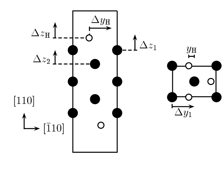
Figure 2: Side (left) and top view (right) of the fully relaxed 5-layer H/Mo (110) system. The solid and empty circles represent Mo- and H-atoms, respectively.

The calculated in-plane lattice constant of 5.91 bohr is used. The $\vec{k}$-integrations are evaluated on a mesh of 64 equally spaced points in the surface Brillouin zone. The MT radii are chosen to be 2.40 bohr and 0.90 bohr for Mo and H, respectively. The kinetic-energy cutoff for the plane wave basis needed for the interstitial region is set to 12 Ry, and the $(l,m)$ representation (inside the MTs) is taken up to $l_{\rm max}=8$ for both Mo and H. Here, the hydrogen MT radius is relatively large compared to that used for the study of the H-dimer. Therefore, a plane-wave cutoff energy of 64 Ry for the representation of the potential is sufficient. The maximum angular momentum of the MT $(l,m)$ expansion of the potential is set to $l_{\rm max}=4$. All states are treated non-relativistically.

In the beginning adsorbate, surface, and subsurface atoms are distorted along the $[\overline{1}10]$ direction with respect to the clean (110) surface configuration in order to break the mirror symmetry of the clean surface. During the relaxation process visualized in Fig. 3

Figure 3: H-Adsorption on Mo(110): Minimization of the total energy for a slab with five Mo-layers. Shown are the distances (in bohr) of the adsorbate and surface atom positions from the optimized structure (left). The respective forces (right) are given in mRy/bohr. The structure parameters $y_{\rm H}$, $z_{\rm H}$, $y_{1}$, and $z_{1}$ are defined in Fig. 2.

all atoms are allowed to move freely perpendicular to the surface and parallel along the $[1\bar{1}0]$-direction. The system is considered to be in a stable or (metastable) geometry when all force components are smaller than $3$ mRy/bohr. The error in the structure parameters of the relaxed system is $\pm 0.02$ bohr.

During the optimization process the hydrogen relaxes into a quasi threefold position with a $[\overline{1}10]$-offset of $y_{\rm H}=1.19$ bohr from the long-bridge position and a height of $d_{\rm H-Mo}=2.04$ bohr above the surface layer. For the surface layer we find a relaxation of $3\pm 0.3\,\%$ of the bulk inter-layer spacing. Furthermore, the surface atoms are slightly distorted by $0.09$ bohr along the $[\overline{1}10]$-direction opposite to the hydrogen with respect to the subsurface. Thus, there is no evidence for a pronounced top-layer-shift reconstruction. The subsurface layer relaxes to its bcc lattice position.

5 Structure of the Program

5.1 Force Calculation

The force implementation fhi95force was developed for WIEN [13] as well as for WIEN93 [25] which is a considerably improved version of the original package. Furthermore, our program is now part of the latest update called WIEN95 [51]. Our intention was to keep the changes related to the original code and the input-files as small as possible. The program and running structure of the program were kept unchanged. In the following, we summarize the basic features of the force computation within WIEN:

• : lapw0
  The electrostatic potential is determined on a logarithmic radial mesh. For the calculation of $\vec{F}_{I}^{\rm HF}$ according to eq. (40) we use the first radial mesh point $r_{I,0}$. Our experience is that $\vec{F}_{I}^{\rm HF}$ behaves numerically stable close to the MT center, i.e., one could also choose $r_{I,1}$ or $r_{I,5}$. Also, the influence of the logarithmic radial mesh chosen is uncritical. The resulting Hellmann-Feynman force $\vec{F}_{I}^{\rm HF}$ is written to unit 70 (case.fhf).

• : lapw1 & lapw2
  The determination of the correction $\vec{F}_{I}^{\rm val}$ is almost completely done in the subroutine l2for (of lapw2) which resembles the original WIEN-subroutine l2main plus the FORTRAN translation of the YSR eqs. (A12), (A17), and (A20). For the evaluation of $\int d\vec{r}^{3}\rho(\vec{r})\nabla V(\vec{r})$ the subroutine fvdrho is called. The only additional input needed is related to the non-spherical matrix elements $\langle u_{l^{\prime}}|V_{\nu}|u_{l}\rangle$, $\langle u_{l^{\prime}}|V_{\nu}|\dot{u}_{l}\rangle$, $\langle\dot{u}_{l^{\prime}}|V_{\nu}|u_{l}\rangle$, and $\langle\dot{u}_{l^{\prime}}|V_{\nu}|\dot{u}_{l}\rangle$ in eq. (A20) of YSR. They are calculated in program lapw1 as a part of the hamiltonian setup and transferred to lapw2 using the input/output unit 71 (case.nsh(s)). The final result $\vec{F}_{I}^{\rm val}$ is written to unit 72 (case.fval or case.fsc). The force calculation which is only executed if the switch FOR instead of TOT is set in case.in2(s) roughly triples the running time of lapw2.

• : core
  The core correction in eq. (38) is calculated by the routine fcore using eq. (2.4). Before that the non-spherical potential has to be read from unit 19 case.vns. Note that $\rho_{\rm core}(\vec{r})$ is spherical. Therefore, only the effective potential parts $V_{lm}^{\rm eff}(r)$ with $l=1$ have to be taken into account. The subroutine fcore uses unit 73 (case.fcor) for the output of $\vec{F}_{I}^{\rm core}$.

• : mixer
  The final step which is the summation of all (available) partial forces according to eq. (36) is done by mixer. This executable writes the accumulated information to unit 70 (case.ftot) and unit 80 (case.finM). The latter can be used as input file for the minimization program mini.

Note that all forces written to the output are in Ry/bohr. Only the calculation of $\vec{F}_{I}^{\rm val}$ can be switched on and off the reason being that the computer time due to $\vec{F}_{I}^{\rm HF}$, $\vec{F}_{I}^{\rm core}$, and the output of the non-spherical matrix elements in lapw1 is negligible. The partial forces $\vec{F}_{I}^{\rm HF}$ and $\vec{F}_{I}^{\rm core}$ are also excellent indicators to monitor the convergence of $\vec{F}_{I}^{\rm val}$ as well as the total atomic force $\vec{F}_{I}$. Therefore, it is convenient to run a self-consistent calculation until $\vec{F}_{I}^{\rm HF}$ or $\vec{F}_{I}^{\rm core}$ are converged and then evaluate $\vec{F}_{I}^{\rm val}$ as a final step. In this way the additional computing time necessary for the atomic forces can be kept at a very low level.

5.2 Minimization

The program mini is executed by invoking the UNIX command ‘mini < mini.def’ in the case-directory. As a first step, the minimization option and the control parameters are read from unit 5 (see Table 1).

NEWT		minimization modus: BFGS/NEWT
0.7 2 2 0		eta, delta(1-3) of atom 1
0.7 1 1 1		eta, delta(1-3) of atom 2
...

Table 1: Input file unit 5 (case.inM)

Then the previous minimization history from unit 16 (case.tmpM) is used to internally generate the approximate inverse Hessian matrix (the velocity coordinate) if the BFGS formalism (damped Newton dynamics scheme) is employed. Now, the calculated total energy and forces are read from unit 15 (case.finM) and used to determine the next trial step. If the new geometry causes an overlap of MT spheres a smaller step along the same direction leading to touching MTs is chosen. Finally, the new trial geometry as well as the updated minimization history are written to unit 21 (case.struct1) and unit 16 (case.tmpM), respectively.

At this point, the FP-LAPW calculation using WIEN for the new geometry can take place. The procedure continues until no further energy minimization can be achieved or all atomic forces fall below a certain minimum.

6 Installation

The program package fhi95force is written in FORTRAN77 and should work on all machines where WIEN can be installed. Because changes of the original code have been kept at a minimum the adaptation of fhi95force to other versions of WIEN and to similar FP-LAPW codes should cause no problems. The extension and the data files are contained in a single tar archive called fhi95force.tar. The extraction on a UNIX machine should generate a directory entitled fhi95force with the following subdirectories:

• SRC_force
  This directory contains the source files of the subroutines which have to be added to the existing code, e.g. lapw0_f.f is the extension for lapw0. (Sub)routines marked with an asterisks in Table 2

  source		routine	relevance for the force calculation
  lapw0_f.f	*	lapw0	calculates and writes Hellmann-Feynman force to unit 70
  lapw1_f.f	*	atpar	writes non-spherical matrix elements to unit 71
  lapw2_f.f		charg2	modification of charge
  		dfrad	obtains radial derivative of a radial function
  	*	lapw2	calls l2for if switch FOR is set
  		l2for	evaluates and writes valence (semi-core) partial forces to unit 72
  		mag	obtains magnitude of a 3-dim vector
  		sevald	computes first derivative of a spline
  		spline	obtains coefficients for cubic interpolation spline
  		vdrho	calculates $\int d^{3}\vec{r}V(\vec{r})\nabla\rho(\vec{r})$
  core_f.f		charge	does Simpson integration inside a sphere
  		dfrad	see lapw2_f.f
  		fcore	calculates core correction of force and writes result to unit 73
  	*	hfsd	calls fcore
  		sevald	see lapw2_f.f
  		spline	see lapw2_f.f
  mixer_f.f	*	mixer	calls totfor
  		totfor	calculates and writes total force to unit 70
  mini.f		dfpmin	minimizes a multi-dimensional function using the BFGS variable metric method
  		finish	writes final output
  		func	reads total energy and atomic forces from unit 15
  		haupt	handles input and output; calls dfpmin or nwtmin
  		inv	evaluates inverse of a matrix
  		latgen	defines lattice (basis vectors)
  		lnsrch	searches for a lower value of a multi-dimensional function along the search direction
  		maxstp	determines maximum possible atomic displacement without overlap of MTs
  		nwtmin	minimizes total energy using damped Newton dynamics
  		pairdis	calculates pair distance of atoms
  		rotate	rotates a vector
  		rotdef	selects symmetry operations of equivalent atoms

  Table 2: Summary of the source files contained in the directory SRC_force. The routines marked with an asterisk already exist in WIEN and have to be updated or substituted by the new versions.

  already exist in the original WIEN code and have to be removed before compiling the program. If the local version of WIEN differs from the original one it should be very easy to update the existing WIEN-routines (lapw0, atpar, lapw2, hfsd, and mixer) by hand. The (few) changes necessary for the force calculations are framed by FORTRAN comment lines (cfb at the beginning and cfe at the end). The compilation with make can be done using existing makefiles which, nevertheless, have to be updated with the additional source files. Before starting a calculation with the new executables it will also be necessary to update the input/output channels according to Table 3.

  executable	unit	I/O	file-name	comment
  lapw0	70	O	case.fhf	Hellmann-Feynman force
  lapw1	71	O	case.nsh(s)	non-spherical matrix elements
  lapw2	2	I	case.in2(s)	input file (switch for force-calculation)
  	19	I	case.vns	non-spherical potential
  	71	I	case.nsh(s)	non-spherical matrix elements
  	72	O	case.f[val/sc]	partial forces due to valence (semi-core) electrons
  core	19	I	case.vns	non-spherical potential
  	73	0	case.fcor	partial force due to core electrons
  mixer	70	O	case.ftot	sum of all available partial forces
  	71	I	case.fhf	Hellmann-Feynman force
  	72	I	case.fval	partial force due to valence electrons
  	73	I	case.fsc	partial force due to semi-core electrons
  	74	I	case.fcor	partial force due to core electrons
  	80	O	case.finM	input file for mini
  mini	5	I	case.inM	input-file
  	6	O	case.outputM	general output-file
  	15	I	case.finM	total energy and atomic forces for current geometry
  	16	I/O	case.tmpM	history of minimization
  	20	I	case.struct	current struct-file
  	21	O	case.struct1	struct-file with new trial geometry

  Table 3: Input and output-files relevant for the force calculation and the minimization procedure.

• SRC_force93
  This is the WIEN93-version of SRC_force.

• SRC_mini
  Here the source for the minimization program can be found. Calling the UNIX command make within the directory creates the executable mini.

• Mo
  This case directory enables the study of the H-point phonon of bcc-Mo similar to the frozen-phonon calculations presented in [20]. It can also be used for testing the minimization program mini.

7 Test run

We recommend to run the Mo test case at the beginning with the already existing local version of WIEN, check the output for warnings and error messages, and than repeat the procedure with the updated WIEN-version setting the FOR switch in Mo.in2 and Mo.in2s.

Then, a step-by-step minimization running alternately WIEN and the new program mini can take place. If this one-dimensional relaxation leads successfully from the distorted to the equilibrium bcc configuration, one may go on to structure optimizations with higher dimensionality.

8 Acknowledgments

This work has benefited from collaborations within, and has been partially funded by, the Network on “Ab-initio (from electronic structure) calculation of complex processes in materials” (contract: ERBCHRXCT930369). We thank P. Blaha, P. Dufek, and K. Schwarz for fruitful discussions and for providing us with the updated version WIEN93 of the WIEN code. Furthermore, we like to acknowledge useful comments by M. Fähnle and contributions of G. Vielsack to the geometry optimization program.

Test run

Output file Mo.force— (starting configuration)

---------
  1.CYCLE
---------
 ja mu      F            |F|             Fx             Fy             Fz

  1  1    >>>   .0000000E+00   .0000000E+00   .0000000E+00   .0000000E+00
---------
  2.CYCLE
---------
 ja mu      F            |F|             Fx             Fy             Fz
  1  1    H-F   .3093266E+01   .0000000E+00   .0000000E+00  -.3093266E+01
  1  1    VAL   .3457794E-01   .8271806E-24   .3308722E-23   .3457794E-01
  1  1    VAL   .1951423E+00  -.3642919E-16  -.5637851E-17   .1951423E+00
  1  1    COR   .2423779E+01   .0000000E+00   .0000000E+00   .2423779E+01

  1  1    >>>   .4397668E+00  -.3642919E-16  -.5637848E-17  -.4397668E+00
...
---------
 11.CYCLE
---------
 ja mu      F            |F|             Fx             Fy             Fz
  1  1    H-F   .1621001E+01   .0000000E+00   .0000000E+00  -.1621001E+01
  1  1    VAL   .1334964E-01   .1654361E-23   .6203855E-24   .1334964E-01
  1  1    VAL   .6451487E-01  -.3089976E-17  -.4201283E-16   .6451487E-01
  1  1    COR   .1409447E+01   .0000000E+00   .0000000E+00   .1409447E+01

  1  1    >>>   .1336895E+00  -.3089974E-17  -.4201283E-16  -.1336895E+00
---------
 12.CYCLE
---------
 ja mu      F            |F|             Fx             Fy             Fz
  1  1    H-F   .1621459E+01   .0000000E+00   .0000000E+00  -.1621459E+01
  1  1    VAL   .1335570E-01  -.4135903E-24  -.1240771E-23   .1335570E-01
  1  1    VAL   .6455603E-01   .3474868E-16  -.9199455E-16   .6455603E-01
  1  1    COR   .1409757E+01   .0000000E+00   .0000000E+00   .1409757E+01

  1  1    >>>   .1337903E+00   .3474868E-16  -.9199455E-16  -.1337903E+00

Output file Mo.tmpM— (after three geometry steps)

  3
    3
           -93.75512         1
   .147750000000D+01   .000000000000D+00         1.4775     .0000     .2500
   .147750000000D+01   .000000000000D+00         1.4775     .0000     .2500
   .159570000000D+01   .668951500000D-01         1.5957     .0669     .2700
           -93.76944         2
   .147750000000D+01   .000000000000D+00         1.4775     .0000     .2500
   .147750000000D+01   .000000000000D+00         1.4775     .0000     .2500
   .152880471000D+01   .284468350000D-01         1.5288     .0284     .2587
           -93.77203         3
   .147750000000D+01   .000000000000D+00         1.4775     .0000     .2500
   .147750000000D+01   .000000000000D+00         1.4775     .0000     .2500
   .145353140400D+01  -.133528500000D-01         1.4535    -.0134     .2459
          .0000000         4
   .147750000000D+01   .000000000000D+00         1.4775     .0000     .2500
   .147750000000D+01   .000000000000D+00         1.4775     .0000     .2500
   .144430222800D+01   .000000000000D+00         1.4443     .0000     .2444

References

- [1] D. D. Koelling, J. Phys. Chem. Solids 33 (1972) 1335; D. D. Koelling and G. O. Arbman, J. Phys. F 5 (1975) 2041.
- [2] O. K. Andersen, Solid State Commun. 13 (1973) 133; Phys. Rev. B 12 (1975) 3060.
- [3] E. Wimmer, H. Krakauer, M. Weinert, and A. J. Freeman, Phys. Rev. B 24 (1981) 864.
- [4] H. J. F. Jansen and A. J. Freeman, Phys. Rev. B 30 (1984) 561.
- [5] L. F. Mattheiss and D. R. Hamann, Phys. Rev. B 33 (1986) 823.
- [6] P. Blaha, K. Schwarz, P. Sorantin, and S. B. Trickey, Comput. Phys. Commun. 59 (1990) 399 .
-
[7]
P. Blaha, K. Schwarz, and R. Augustyn,
WIEN93 (Technical University, Vienna, 1993);
improved and updated UNIX version of the original copyrighted
WIEN-code [6]. - [8] D. J. Singh, Planewaves, pseudopotentials and the LAPW method (Kluwer Academic, Boston, 1994).
- [9] R. Yu, D. Singh, and H. Krakauer, Phys. Rev. B 43 (1991) 6411.
- [10] R. Stumpf and M. Scheffler, Comp. Phys. Commun. 79 (1994) 447.
- [11] C. G. Broyden, J. E. Dennis, and J. J. Moré, J. Inst. Maths. Appl. 12, 223 (1973).
- [12] K. W. Brodlie, in The State of the Art in Numerical Analysis, ed. D. A. H. Jacobs (Academic Press, London, 1977).
- [13] J. E. Dennis and R. B. Schnabel, Numerical Methods for Unconstrained Optimization and Nonlinear Equations (Prentice-Hall, Englewoods Cliffs, 1983).
- [14] B. Kohler, P. Ruggerone, S. Wilke, and M. Scheffler, Phys. Rev. Lett. 74 (1995) 1387.
- [15] S. Wilke and M. Scheffler, SS329 (1995) L605.

References

- [1] J. C. Slater, Phys. Rev. 51 (1937) 846.
- [2] J. C. Slater, Advances in Quantum Chemistry 1 (1964) 35.
- [3] T. L. Loucks, Augmented Plane Wave Method (Benjamin, New York, 1967).
- [4] L. F. Mattheiss, J. H. Wood, and A. C. Switendick, Meth. Comp. Phys 8 (1968) 64.
- [5] J. O. Dimmock, Solid State Phys. 26 (1971) 103.
- [6] H. Bross, Phys. Kondens. Mater. 3 (1964) 119; Z. Phys. B 81 (1990) 233.
- [7] P. Marcus, Int. J. Quantum. Chem. Suppl. 1 (1967) 567.
- [8] D. D. Koelling, J. Phys. Chem. Solids 33 (1972) 1335; D. D. Koelling and G. O. Arbman, J. Phys. F 5 (1975) 2041.
- [9] O. K. Andersen, Solid State Commun. 13 (1973) 133; Phys. Rev. B 12 (1975) 3060.
- [10] E. Wimmer, H. Krakauer, M. Weinert, and A. J. Freeman, Phys. Rev. B 24 (1981) 864.
- [11] H. J. F. Jansen and A. J. Freeman, Phys. Rev. B 30 (1984) 561.
- [12] L. F. Mattheiss and D. R. Hamann, Phys. Rev. B 33 (1986) 823.
- [13] P. Blaha, K. Schwarz, P. Sorantin, and S. B. Trickey, Comput. Phys. Commun. 59 (1990) 399.
- [14] D. J. Singh, Planewaves, pseudopotentials and the LAPW method (Kluwer Academic, Boston, 1994).
- [15] P. Blaha, K. Schwarz, and P. Herzig, Phys. Rev. Lett. 54 (1985) 1192.
- [16] B. Kohler, M. Fuchs, K. Freihube, and M. Scheffler, Phys. Rev. A 49 (1994) 5152.
- [17] P. Blaha, K. Schwarz, P. Dufek, G. Vielsack, and W. Weber, Z. Naturforsch. 48a (1993) 129.
- [18] B. Kohler, P. Ruggerone, S. Wilke, and M. Scheffler, Phys. Rev. Lett. 74 (1995) 1387; in: Electronic Surface and Interface States on Metallic Systems, eds. E. Bertel and M. Donath (World Scientific, Singapore, 1995).
- [19] J. M. Soler and A. R. Williams, Phys. Rev. B 40 (1989) 1560; Phys. Rev. B 42 (1990) 9728.
- [20] R. Yu, D. Singh, and H. Krakauer, Phys. Rev. B 43 (1991) 6411.
- [21] R. Yu, H. Krakauer, and D. Singh, Phys. Rev. B 45 (1992) 8671.
- [22] S. Goedecker and K. Maschke, Phys. Rev. B 45 (1992) 1597.
- [23] H. G. Krimmel, J. Ehmann, C. Elsässer, M. Fähnle, and J. M. Soler, Phys. Rev. B 50 (1994) 8846.
- [24] M. Fähnle, C. Elsässer, and H. Krimmel, submitted to Physica Status Solidi B.
-
[25]
P. Blaha, K. Schwarz, and R. Augustyn,
WIEN93(Technical University, Vienna, 1993); improved and updated UNIX version of the original copyrightedWIEN-code [13]. - [26] P. Hohenberg and W. Kohn, Phys. Rev. 136 (1964) B864.
- [27] W. Kohn and L. J. Sham, Phys. Rev. 140 (1965) A1133.
- [28] M. J. Gillan, J. Phys. Condens. Matter 1 (1989) 689.
- [29] J. Neugebauer and M. Scheffler, Phys. Rev. B 46 (1992) 16067.
- [30] W. Weinert and J. W. Davenport, Phys. Rev. B 45 (1992) 13709.
- [31] H. Hellmann, Einführung in die Quantenchemie (Deuieke, Leipzig,1937) p. 285.
- [32] R. P. Feynman, Phys. Rev. 56 (1939) 340.
- [33] D. G. Pettifor, Commun. Phys. 1 (1976) 141; J. Phys. F 8 (1978) 219.
- [34] O. K. Andersen, O. Jepsen, and D .Glötzel, in: Highlights of Condensed-Matter Theory, ed. F. Bassani, F. Fumi, and M. P. Tosi (North Holland, Amsterdam, 1985) p. 59.
- [35] M. Methfessel and M. van Schilfgaarde, Phys. Rev. B 48 (1993) 4937.
- [36] P. Pulay, Mol. Phys. 17 (1969) 197.
- [37] C. Satoko, Chem. Phys. Lett. 83 (1981) 111; Phys. Rev. B 30 (1984) 1754.
- [38] P. Bendt and A. Zunger, Phys. Rev. Lett. 50 (1983) 1684.
- [39] M. Scheffler, J. P. Vigneron, G. B. Bachelet, Phys. Rev. B 31 (1985) 6541.
- [40] A. C. Hurley, Proc. Roy. Soc. London, Ser. A 260 (1954) 379.
- [41] J. M. Soler and A. R. Williams, Phys. Rev. B 47 (1993) 6784.
- [42] M. Weinert, J. Math. Phys. 22 (1981) 2433.
- [43] G. Arfken, Mathematical methods for physicists (Academic Press, San Diego, 1985) p. 699.
- [44] C. G. Broyden, J. E. Dennis, and J. J. Moré, J. Inst. Maths. Appl. 12 (1973) 223.
- [45] K. W. Brodlie, in The State of the Art in Numerical Analysis, ed. D. A. H. Jacobs (Academic Press, London, 1977).
- [46] J. E. Dennis and R. B. Schnabel, Numerical Methods for Unconstrained Optimization and Nonlinear Equations (Prentice-Hall, Englewoods Cliffs, 1983).
- [47] W. H. Press, S. A. Teukolsky, W. T. Vetterling, and B. P. Flannery, Numerical Recipes in FORTRAN: the art of scientific computing (Cambridge University Press, Cambridge, 1992).
- [48] R. Stumpf and M. Scheffler, Comp. Phys. Commun. 79 (1994) 447.
- [49] J. P. Perdew, J. A. Chevary, S. H. Vosko, K. A. Jackson, M. R. Pederson, D. J. Singh, and C. Fiolhais, Phys. Rev. B 46 (1992) 6671.
- [50] M. Altman, J. W. Chung, P. J. Estrup, J. M. Kosterlitz, J. Prybyla, D. Sahu, and S. C. Ying, J. Vac. Sci. Technol. A 5 (1987) 1045.
-
[51]
P. Blaha, K. Schwarz, P. Dufek, and R. Augustyn,
WIEN95(Technical University, Vienna, 1995); improved and updated UNIX version of the original copyrightedWIEN-code [13].