Persistence of Invariant Manifolds for Nonlinear PDEs

Abstract

We prove that under certain stability and smoothing properties of the semi-groups generated by the partial differential equations that we consider, manifolds left invariant by these flows persist under $C^{1}$ perturbation. In particular, we extend well known finite-dimensional results to the setting of an infinite-dimensional Hilbert manifold with a semi-group that leaves a submanifold invariant. We then study the persistence of global unstable manifolds of hyperbolic fixed-points, and as an application consider the two-dimensional Navier-Stokes equation under a fully discrete approximation. Finally, we apply our theory to the persistence of inertial manifolds for those PDEs which possess them.

1 Introduction

We consider a nonlinear partial differential equation which takes the form of an evolution equation having infinite-dimensional Riemannian manifold $X$ as its configuration space. We assume that this PDE generates a $C^{1}$ nonlinear semi-group $S(t)$ which leaves a $C^{r}$ differentiable compact submanifold with boundary $\overline{M}$ either overflowing or inflowing invariant, and examine the persistence of this submanifold under small $C^{1}$ perturbations of $S(t)$ in a neighborhood of $\overline{M}$. Specifically, we prove that if a semi-group ${S^{\nu}}(t)$ is within a ${\nu}$-diameter $C^{1}$ ball about $S(t)$, and if the submanifold $\overline{M}$ is normally hyperbolic, attracting trajectories at an exponential rate, with a rate of attraction in the normal direction greater than in the tangential direction, a continuously differentiable invariant submanifold with boundary of the same type $\overline{M_{\nu}}$ exists for ${S^{\nu}}(t)$ and converges to $\overline{M}$ as ${\nu}$ tends to zero. Our result generalizes the persistence theory for manifolds invariant to finite-dimensional vector fields that has been studied by Moser, Sacker, Hirsh, Pugh, & Shub, and Fenichel (see [44], [49], [30] and [19]). Unlike the flows generated by differentiable finite-dimensional vector fields, however, the semi-group $S(t)$ does not, in general, possess a bounded inverse and hence, for fixed $t$, the map $S(t)$ is not a diffeomorphism. In particular, its inverse is only defined on the invariant manifold. Furthermore, the configuration space is not locally compact, so that one must strongly rely on the $C^{1}$ regularity of the map together with the compactness of $\overline{M}$ to establish important local bounds.

Recently, Bates, Lu, & Zeng (see [4]) have generalized the finite-dimensional persistence theory of Hirsh, Pugh, & Shub to semiflows in Banach spaces; in our notation, their configuration space $X$ is a Banach vector space. They consider compact manifolds $M$ without boundary as having center-type flow, and are able to prove the persistence result for both stable-center and the more difficult unstable-center case, the latter being quite complicated due to the general lack of backwards-in-time flow. Herein, our main interest is in applying the general persistence theory to global unstable manifolds and inertial manifolds associated with nonlinear partial differential equations, so we will restrict our attention to the case of stable flow in the infinite-dimensional Riemannian manifold.

We remark that our choice of a Hilbert manifold for the configuration space may be attributed to the following reasons. First, we must require the existence of a second order vector field or spray on $X$ which generates the geodesic flow. In general, Banach spaces are not separable so that an infinite-dimensional manifold modeled on a Banach space may not be paracompact and hence may not have global partitions of unity. Since it is essential for us to be able to construct tubular neighborhoods about our embedded submanifold $\overline{M}$ (we describe these in the next section), we must require geodesics on $X$ to exist. In the Hilbert manifold setting, the existence of such geodesic flows is equivalent to the existence of a Lagrangian vector field associated with the kinetic energy Lagrangian. The Riemannian structure generates a natural symplectic form on $T^{*}X$ which is only weakly nondegenerate, meaning that the associated linear map taking vector fields to $1$-forms is generally not surjective. It is, nevertheless, possible to confirm that the Hilbert manifolds common to most applications do indeed possess geodesics, and herein we shall restrict our attention to such examples. A classical example of a configuration manifold which does not have linear structure arises in fluids applications. If one is interested in perfect incompressible fluid flow governed by the Euler equations, then the approriate configuration space is the closure of the volume preserving diffeomorphisms under a Hilbert space norm, a Hilbert manifold (see [17]). Our examination of the persistence problem for this PDE shall appear in a future work. Another interesting example is the Sine-Gordon equation whose fields take values in ${\mathbb{S}}^{1}$. One could argue that the analysis of this PDE could be trivially done by working in the universal covering space, however, if one is interested in the perturbation of invariant manifolds, and wishes to work in the linear space supplied by the cover, one would then have to prove that the perturbed structure remains an invariant manifold after projecting from the covering space back to the quotient.

Another reason for choosing a Hilbert space structure is that we may reduce the normal bundle of the invariant manifold $\overline{M}$ to a Hilbert or unitary bundle, wherein the transition maps are unitary. This is essential for the local analysis that we perform.

Recall that an overflowing (inflowing) invariant manifold with boundary $\overline{M}$ satisfies $S(t)u\in\overline{M}$ for any $u\in\overline{M}$ for all $t<0$ ($t>0$). This means that the infinite-dimensional vector field defined by the partial differential operator points outward (inward) on the boundary of the manifold. The existence of such an overflowing (inflowing) invariant manifold $\overline{M_{\nu}}$ for the perturbed semi-group ${S^{\nu}}(t)$ is established by standard contraction mapping arguments. Specifically, after diffeomorphically identifying the infinite-dimensional manifold $X$ with the normal bundle over $\overline{M}$ in a neighborhood $V$ of $\overline{M}$, we search for $\overline{M_{\nu}}$ in the space of sections of this normal bundle. The invariant manifold is the image of the particular section which is the fixed-point for each time-$t$ map ${S^{\nu}}(t)$. We remark that Fenichel’s proof in finite dimensions in its local form essentially works for the infinite-dimensional vector bundle setting with minor modifications, especially for showing that the persisting manifold is Lipschitz. We provide a different proof, however, that the persisting manifold is actually continuously differentiable.

As an application of our persistence theorem, we show that the unstable manifold of a hyperbolic fixed-point of a PDE satisfies the conditions sufficient for persistence so that the approximating semi-group possesses a continuously differentiable unstable manifold of its hyperbolic fixed-point which uniformly converges to the unstable manifold of the unperturbed system (see [43] for a proof using the deformation method for perturbation of the linearized system). We may then deduce, following the work of [29], that the global unstable manifold of the obtained stationary solution, defined by evolving the perturbed local unstable manifold forward in time, is lower semi-continuous. In case the global attractor is the closure of the unstable manifolds (of overflowing manifolds) such as with gradient systems, we find that the attractor is lower semi-continuous as well.

As the majority of nonlinear PDEs generate semi-groups which have no explicit representation, it is of great interest to consider numerical schemes as the $C^{1}$ close approximations of the semi-group. In fact, our motivation for perturbing the semi-group rather than the PDE may primarily be attributed to the inability of numerical schemes to approximate infinite-dimensional vector fields in a $C^{1}$ sense. As an application, we show that the unstable manifold of the hyperbolic stationary solution to the 2D Navier-Stokes equation persists under a fully discrete numerical approximation.

Next we apply our theory to the persistence of inertial manifolds for those PDEs that possess them. An inertial manifold for a PDE is a smooth finite-dimensional, exponentially attracting, positively invariant manifold containing the global attractor (see [21], [22]). Subsequent works extended the existence results to more general equations and provided alternative methods of proof (see for example [48] and the references therein). Most existence proofs require a gap condition to hold in the spectrum of the linear term. As shown in [48], this gap condition also insures that the inertial manifold is normally hyperbolic. Thus, our persistence theory applies to PDEs satisfying this gap condition; however, since our theory is local, we may only conclude that the perturbed system possesses an inflowing manifold that is close to the inertial manifold. In particular, the inflowing manifold for the perturbed system may not globally exponentially attract all trajectories, as often occurs when discretizing dissipative systems. We include cases where the inflowing manifold is an inertial manifold for the perturbed system.

Our applications complement existing results relating the long-time dynamics of PDEs to the long-time dynamics of their numerical approximations as the time and space mesh are refined. In [13], [55] sufficient conditions are found on a Galerkin scheme approximating the Navier-Stokes equations (NSE) to infer the existence of a nearby stable stationary solution for the NSE from the apparent stability of the time-dependent Galerkin approximate solutions. Stable periodic orbits are studied in [56], while hyperbolic periodic orbits can be found in [2]. Other aspects of the large-time behavior of the Galerkin approximation to the exact solutions of the NSE are considered in [28]; subsequent results examined the behavior of solutions near equilibria of PDEs under numerical perturbation (see [52], [1], [37]). For more general global attractors, see [26] for sufficient conditions on upper semi-continuity. For persistence of inertial manifolds under numerical approximation, see [22], [23], [14], [24], [33], and [34].

We structure the paper in the following way. In Section 2, we prove that if a nonlinear PDE has an overflowing invariant manifold that is normally hyperbolic and whose semi-group satisfies certain regularity conditions, then a continuously differentiable overflowing invariant manifold persists under $C^{1}$ perturbation of the semi-group. In Section 3, we state the general form of the nonlinear partial differential equation and define the domain of the semi-group which it generates. In Section 4, we prove that the global unstable manifold of a hyperbolic fixed-point (of the PDE described in Section 3) persists as a continuously differentiable overflowing invariant manifold. We apply this result to the examination of the two-dimensional Navier-Stokes equation in Section 5, and finally, in Section 6, we prove that inertial manifolds persist as well.

2 Construction of the perturbed manifold

In this section, we generalize Fenichel’s proof of the persistence of overflowing invariant manifolds to the setting of an infinite dimensional Riemannian manifold. Much of the proof goes through essentially unchanged, particularly the portion which shows that the persisting manifold is Lipschitz continuous; however, we provide a complete exposition in order to account for the changes required in infinite dimensions, as well as to clarify and generalize some of the details in the technical lemmas. As for the final result that the persisting manifold is actually $C^{1}$, we take a different approach than Fenichel, and show that the persisting manifold is a limit of a $C^{1}$ Cauchy sequence.

2.1 Infinite-dimensional geometry and sufficient conditions for persistence

Let $(X,g)$ be an infinite-dimensional $C^{r}$ Riemannian manifold modeled on a Hilbert space $({\mathbb{H}},\langle\cdot,\cdot\rangle)$, where $r\geq 3$. We consider a $C^{1}$ injective map $S:X{\rightarrow}X$ which leaves a submanifold with boundary $\overline{M}$ negatively invariant and has an inverse defined on $\overline{M}$. In particular, we assume the existence of a compact, connected, and embedded $C^{r}$ submanifold $\overline{M}=M\cup\partial M$ such that $S^{-1}(\overline{M})\subset\overline{M}$. We further assume that $\overline{M}\subset M^{\prime}$, where $M^{\prime}$ is also a $C^{r}$ connected and embedded submanifold of $X$ having compact closure, which is the same dimension as $M$ and satisfies ${S^{-1}}(M^{\prime})\subset\overline{M}$. This gives each $x\in\overline{M}$ an $M^{\prime}$-open neighborhood, and thus allows us to avoid the complications associated with charts defined on domains with boundary. We assume that the differential of $S^{-1}|_{M^{\prime}}$ is only defined in the tangent bundle of $M^{\prime}$ rather than in the entire tangent bundle of $X$ over $M^{\prime}$.

We consider the tangent bundle $(T(X),\pi)$ restricted to $\pi^{-1}(M^{\prime})$ and use its Riemannian structure to induce the splitting

$$T(X)|_{M^{\prime}}=T(M^{\prime})\oplus N,$$

where $N$ is the $C^{r-1}$ normal bundle (any transverse bundle). It is implicit in our compactness assumption that $\overline{M^{\prime}}$ is finite dimensional, and for concreteness, we fix the dimension to be $m$. Due to the local trivialization of the vector bundles, there exists an open covering consisting of $M^{\prime}$-open sets ${\mathcal{U}}=\{U_{i},i\in{\mathcal{I}}\}$ of $\overline{M}$, such that for each $U_{i}\in{\mathcal{U}}$, we have the vector bundle morphisms

$$\tau^{M^{\prime}}_{i}:T(M^{\prime})|_{U_{i}}{\rightarrow}U_{i}\times{\mathbb{P}},\ \ \ \tau^{N}_{i}:N|_{U_{i}}{\rightarrow}U_{i}\times{\mathbb{Q}},$$

where ${\mathbb{H}}={\mathbb{P}}\oplus{\mathbb{Q}}$. In fact, due to the compactness of $\overline{M}$, for any such trivializing open cover ${\mathcal{U}}$, we may choose finite refined subcovers on which we can define charts:

$$({\mathcal{U}}^{j}=\{U_{i}^{j},i=1,...,s\},\sigma_{i}),j=1,...,J,\ \ U^{1}_{i}\subset\overline{U_{i}^{1}}\subset\cdot\cdot\cdot\subset U^{J-1}_{i}\subset\overline{U^{J-1}_{i}}\subset U^{J}_{i}\subset\overline{U^{J}_{i}}$$

and $\sigma_{i}(U_{i}^{j})={\mathcal{B}}_{j}(0)$, the ball of radius $j$ centered about the origin in ${\mathbb{P}}$. We simply choose for each $x\in\overline{M}$ a chart $(W_{x},\sigma_{x})$ such that $W_{x}\subset U_{i}\in{\mathcal{U}}$ and ${\mathcal{B}}_{J}(0)\subset\sigma_{x}(W_{x})$ and then define $U_{x}^{j}\equiv\sigma_{x}^{-1}({\mathcal{B}}_{j}(0))$, and extract the finite cover. Thus, for each $i$ and any $p\in U^{j}_{i}$, $\sigma_{i}(p)$ is an $m$-vector spanned by the first $m$ elements of a fixed ordered basis of ${\mathbb{H}}$.

For the purpose of defining small local neighborhoods in the normal bundle, it will be convenient to consider the reduction of $(N,\pi|_{N})$ to the Hilbert group. Recall, that $Hilb({\mathbb{Q}})$ is the subgroup of $Laut({\mathbb{Q}})$ which preserves the inner product, so that a linear automorphism $I$ is in $Hilb({\mathbb{Q}})$ if and only if $I^{*}I=Id$ on ${\mathbb{Q}}$. Given our Riemannian metric $g$, we may construct the Hilbert trivializations from our vector bundle trivializations $(U_{i}^{j},\tau^{N}_{i})$. Namely, for each $x\in U_{i}^{j}$ and any $q_{1}$, $q_{2}$ in ${\mathbb{Q}}$, there exists a positive definite symmetric operator $T_{ix}$ satisfying $g_{ix}(q_{1},q_{2})=\langle T_{ix}q_{1},q_{2}\rangle$. Then, the Hilbert trivialization is defined for each $i$ by $(U_{i}^{j},\overline{\tau}_{i})$, where $\overline{\tau}_{i}=T_{ix}^{\frac{1}{2}}\tau^{N}_{ix}$. We have defined our Hilbert trivializations over the open covers $\cup_{i=1}^{s}U^{j}_{i}$ of $\overline{M}$; thus, any continuous map defined on some $\cup_{i=1}^{s}U^{j}_{i}$ can be uniformly bounded when restricted to $\cup_{i=1}^{s}\overline{U^{j-1}_{i}}$. Often, we will use such compact refinements as domains of sections and operators.

Henceforth, $N$ will represent the reduction of the normal vector bundle to the Hilbert group. We define the bounded subset of the normal Hilbert bundle:

$$N^{\varepsilon}=\{v\in N_{x}:g_{x}(v,v)<{\varepsilon}^{2},\ x\in M^{\prime}\}.$$

$N^{\varepsilon}$ defines an open neighborhood of the zero section of the normal Hilbert bundle; the set of locally Lipschitz sections of this neighborhood $N^{\varepsilon}$ will contain the negatively invariant manifold of the perturbed map ${S^{\nu}}$ upon identification of an open neighborhood of $\overline{M^{\prime}}$ with $N^{\varepsilon}$. This identification is given by the existence of a tubular neighborhood diffeomorphism $h$ taking $N^{\varepsilon}$, for ${\varepsilon}$ sufficiently small, onto $V$, where $V$ is some $X$-open neighborhood of $\overline{M^{\prime}}$.

Lemma 2.1

Let $X$ be a $C^{r}$ manifold, $r\geq 3$, that admits a partition of unity and let ${\mathcal{M}}$ be a closed submanifold. Then there exists a tubular neighborhood of ${\mathcal{M}}$ in $X$ of class $C^{r-2}$.

This result is well known and can be found in most texts on infinite-dimensional manifolds (see [36] for example). Of course our Hilbert manifold has partitions of unity since the norm is differentiable; furthermore, we have a canonical spray whose geodesic field on $T(X)$ defines the exponential map $exp$. In other words, we require the Lagrangian vector field associated with the kinetic energy of the metric to exist. In general, for infinite-dimensional Riemannian manifolds, the metric is only weakly nondegenerate, but we will restrict attention to model Hilbert spaces which are isomorphic to their dual space. The map $h$ is simply the restriction of the exponential to the normal bundle, $h=exp|_{N}$. Because $h$ is at least a diffeomorphism of class $C^{1}$, there exists a constant $C$ such that $\|Dh\|<C$ and $\|Dh^{-1}\|<C$ on $\overline{V}$. In case that $C>1$, we will use this constant in certain global estimates, so that it may disappear in the local versions of these estimates. We take our closed submanifold ${\mathcal{M}}$ in Lemma 2.1 to be $\overline{M^{\prime}}$, and let $\overline{S}\equiv h^{-1}\circ S\circ h$.

We note that in many of the applications that we have in mind, the manifold $X$ is itself a Hilbert space, in which case $X$ is identified with $T(X)$ and the geodesic field is trivial. In that instance, the tubular neighborhood is obtained from the smooth diffeomorphism $h:N^{\varepsilon}{\rightarrow}X$ defined by $(x,v)\mapsto x+v$ and we may relax our regularity to $r\geq 2$. In fact, if we are content with continuous vector bundles over $\overline{M}$, we may take $r\geq 1$.

Definition 2.2

Denote by $P$ and $Q$ the following projection operators:

$$P:T(X)|_{M^{\prime}}{\rightarrow}T(M^{\prime}),\text{ and }Q:T(X)|_{M^{\prime}}{\rightarrow}N.$$

We will need the following stability condition on our negatively invariant submanifold.

Condition 2.3 (Stability)

Let $B(p)\equiv Q\circ DS(S^{-1}(p))|_{N}:N_{S^{-1}(p)}{\rightarrow}N_{p}$, and let $\vartheta_{1}\in(0,1)$. Then $C^{2}\|B(p)\|<\vartheta_{1}$ for all $p\in\cup_{i=1}^{s}\overline{U_{i}^{J-1}}.$

This requirement simply states that to first order, the map $S$ decreases lengths of vectors along the normal bundle fibers by at least a factor of $C^{2}\vartheta_{1}^{-1}$. We show that this implies that the map $S$ sends elements of the tubular neighborhood about $S^{-1}(M)\subset M$ “closer” to $M$.

Lemma 2.4

For $0<{\varepsilon}<{\varepsilon}_{0}$ sufficiently small, $\overline{S}:N^{\varepsilon}|_{S^{-1}(\overline{U_{i}^{J-2}})}{\rightarrow}N^{C^{-2}\vartheta_{2}{\varepsilon}}|_{U_{i}^{J-1}}$ for some $\vartheta_{2}\in(\vartheta_{1},1)$.

Proof.

By definition of our tubular neighborhood, every $p\in M$ has a normal neighborhood $R_{p}$ diffeomorphic to ${\mathcal{B}}_{\varepsilon}(0)$ in $T_{p}X$. Let $p\in\overline{U_{i}^{J-2}}$, and let $v\in N^{\varepsilon}|_{S^{-1}(p)}$. By continuity, we may choose ${\varepsilon}$ small enough such that $h(v)\in R_{S^{-1}(p)}$ and $S(h(v))\in R_{p}$. Since $exp_{p}^{-1}\circ S\circ h$ is at least a $C^{1}$ map taking ${\mathcal{B}}_{\varepsilon}(0)\subset T_{S^{-1}(p)}X$ into $T_{p}X$, it differs from the linear map $DS_{S^{-1}(p)}v$ by ${\mathcal{O}}(\|v\|^{2})$ terms using Taylor’s theorem, and thus by ${\mathcal{O}}({\varepsilon}^{2})$.

By projecting $exp_{p}^{-1}\circ S\circ h$ onto $N$ and using Condition 2.3, we may choose ${\varepsilon}$ small enough so that $C^{-2}\vartheta_{1}{\varepsilon}+{\mathcal{O}}({\varepsilon}^{2})<C^{-2}\vartheta_{2}{\varepsilon}$, since $C>1$. Then, there exists some $p^{\prime}\in R_{p}\cap M$ such that $\|(exp|_{N})^{-1}|_{p^{\prime}}(S(h(v)))\|=\|Q\ exp_{p}^{-1}(S(h(v)))\|$. Using the compactness of $\overline{U_{i}^{J-2}}$, we may pick an ${\varepsilon}_{0}$ small enough which holds for any $p\in\overline{U_{i}^{J-2}}$.  $\blacksquare$

We will use the local Hilbert bundle trivializations that we have constructed to associate to each section restricted to some $U^{j}_{i}$ a $graph$ over ${\mathcal{B}}_{j}(0)$ in ${\mathbb{P}}\times{\mathbb{Q}}$. This will allow us to compare elements from distinct fibers without using parallel translation. For each $i\in\{1,...,s\}$ and $p\in U^{J}_{i}$ and $q\in N^{\varepsilon}_{x}$, define $\psi_{i}$ by letting

$$\overline{\tau}_{i}(p,q)=(\pi|_{N}(p,q),\psi_{i}(p,q))=(p,{\psi_{i}}_{p}(q)),$$ (2.1)

where ${\psi_{i}}_{p}(q)\in{\mathbb{Q}}$. We denote by ${\mathcal{S}}^{\varepsilon}$ the sections of $N^{\varepsilon}$ restricted to the cover ${\mathcal{U}}^{J-3}$, i.e. ${\mathcal{S}}^{\varepsilon}={\Gamma(N^{\varepsilon}|_{\cup_{i=1}^{s}U^{J-3}_{i}})}$. Then for all $u\in{\mathcal{S}}^{\varepsilon}$, we may correspond to $u|_{U^{J-3}_{i}}$ the map $u_{i}:B_{J-3}(0)\subset{\mathbb{P}}{\rightarrow}{\mathbb{Q}}$ defined by $u_{i}=\psi_{i}\circ u\circ\sigma_{i}^{-1}$. For any two elements $v,w\in{\mathcal{S}}^{\varepsilon}$, $v$ and $w$ are $\epsilon$-$C^{0}$ close if

$$\|v-w\|_{0}:=\max_{1\leq i\leq s}\sup_{x\in{\mathcal{B}}_{J-3}(0)}\|v_{i}(x)-w_{i}(x)\|\leq\epsilon.$$

We define

$$Lip(u)=\max_{1\leq i\leq s}\sup_{z,z^{\prime}\in{\mathcal{B}}_{J-3}(0)}\frac{\|u_{i}(z)-u_{i}(z^{\prime})\|}{\|z-z^{\prime}\|}$$

if it exists, and let ${\mathcal{S}}^{\varepsilon}_{\delta}=\{u\in{\mathcal{S}}^{\varepsilon}:Lip(u)\leq\delta\}$. Then, for any $u\in{\mathcal{S}}^{\varepsilon}_{\delta}$, $h\circ Im(u)$ is a Lipschitz continuous manifold of dimension $m$. It is important to note that in any chart overlap $U^{J-3}_{i}\cap U^{J-3}_{k}$, $i,k\in\{1,...,s\}$,

$$\sup_{z,z^{\prime}\in\sigma_{i}(U^{J-3}_{i})\cap\sigma_{k}(U^{J-3}_{k})}\frac{\|u_{i}(z)-u_{i}(z^{\prime})\|}{\|z-z^{\prime}\|}<\infty\Longrightarrow\sup_{z,z^{\prime}\in\sigma_{i}(U^{J-3}_{i})\cap\sigma_{k}(U^{J-3}_{k})}\frac{\|u_{k}(z)-u_{k}(z^{\prime})\|}{\|z-z^{\prime}\|}<\infty.$$

Indeed, because of our reduction to the Hilbert group, there exists a $C^{r-1}$ Hilbert automorphism $O_{ki}$ on any overlap region $U^{J-3}_{i}\cap U^{J-3}_{k}$ so that

$$\psi_{k}(Im(u|_{U^{J-3}_{i}\cap U^{J-3}_{k}}))=O_{ki}\ \psi_{i}(Im(u|_{U^{J-3}_{i}\cap U^{J-3}_{k}})),$$

and since we were careful to shrink our patches, these Hilbert maps are also Lipschitz in the operator norm topology. This is a slight generalization of the finite-dimensional setting wherein on requires each element of an orthonormal basis to be a $C^{r-1}$ function over each patch, and then relies on the equivalence of norms to conclude that the frame is $C^{r-1}$.

Finally, let $v,w\in{\mathcal{S}}^{\varepsilon}$ be continuously differentiable, and to each such section $v$ associate the $s$-vector of linear operators $(Dv_{1},...,Dv_{s})$ where

$$Dv_{i}\in C^{0}({\mathcal{B}}_{J-3}(0),{\mathcal{L}}({\mathbb{P}},{\mathbb{Q}}))\ \ \mbox{for}\ \ i=1,...s.$$

Then, $v$ and $w$ are $\epsilon$-$C^{1}$ close if they are $\epsilon$-$C^{0}$ close and

$$\|Dv-Dw\|\equiv\max_{i}\sup_{x\in{\mathcal{B}}_{J-3}(0)}\|Dv_{i}(x)-Dw_{i}(x)\|\leq\epsilon.$$

Definition 2.5

Let $S^{\nu}:X{\rightarrow}X$ be ${\nu}$-$C^{1}$ close to $S$ on $V$, and define $\overline{S^{\nu}}\equiv h^{-1}\circ S^{\nu}\circ h$.

Corollary 2.6

For $0<{\varepsilon}<{\varepsilon}_{0}$ and ${\nu}>0$ both sufficiently small,

$$\overline{S^{\nu}}:N^{\varepsilon}|_{S^{-1}(\overline{U_{i}^{J-2}})}{\rightarrow}N^{\varepsilon}|_{U_{i}^{J-1}}.$$

Proof.

This immediately follows from Definition 2.5 and Lemma 2.4.  $\blacksquare$

Following [19], we will use the implicit function theorem to show that the images of Lipschitz sections of $N^{\varepsilon}$ under $\overline{S^{\nu}}$ remain sections of the bundle.

Lemma 2.7

For $\delta$, ${\nu}$, and ${\varepsilon}$ taken sufficiently small, $\overline{S^{\nu}}:{\mathcal{S}}^{\varepsilon}_{\delta}{\rightarrow}{\mathcal{S}}^{\varepsilon}$.

Proof.

The fact that ${S^{-1}}(\cup_{i=1}^{s}U_{i}^{J-1})\subset M$ and ${S^{-1}}(M)\subset\overline{M^{\prime}}\subset\cup_{i=1}^{s}U_{i}^{J-3}$ together with Corollary 2.6 ensures that the maps $\chi(p;{\varepsilon},{\nu},\delta)\equiv\pi|_{N}\circ\overline{S^{\nu}}\circ u\circ S^{-1}(p)$ are well defined for all $u\in{\mathcal{S}}^{\varepsilon}_{\delta}$ and all $p\in\cup U^{J-2}_{i}$.

We must show that these maps are injective. In any patch $U^{J-1}_{i}$, we define the local representative of $\chi$ to be $\chi_{i}({\varepsilon},{\nu},\delta)=\sigma_{i}\circ\chi(\cdot;{\varepsilon},{\nu},\delta)|_{U^{J-1}_{i}}\circ\sigma_{i}^{-1}$, and note that $\chi_{i}(0,0,\delta)$ is the inclusion map of ${\mathcal{B}}_{J-2}(0)$ into ${\mathbb{P}}$. By the implicit function theorem for Lipschitz continuous maps (see [16]), there exists a neighborhood ${\mathcal{X}}$ of $\chi_{i}(0,0,\delta)$ in the Lipschitz topology such that each $f\in{\mathcal{X}}$ maps ${\mathcal{B}}_{J-2}(0)$ into ${\mathbb{P}}$ injectively and satisfies

$$\overline{{\mathcal{B}}_{J-3}(0)}\subset f({\mathcal{B}}_{J-2}(0))\subset\overline{f({\mathcal{B}}_{J-2}(0))}\subset{\mathcal{B}}_{J-1}(0).$$

To each $f\in{\mathcal{X}}$ we identify the injective map $\bar{f}$ on $U_{i}^{J-1}$ and have

$$\overline{U_{i}^{J-3}}\subset\bar{f}(U_{i}^{J-2})\subset\overline{\bar{f}(U_{i}^{J-2})}\subset U_{i}^{J-1}.$$ (2.2)

By taking ${\varepsilon}$, $\delta$, and ${\nu}$ small enough, $\chi_{i}({\varepsilon},{\nu},\delta)$ can be made arbitrarily close to the inclusion map and thus is an element of ${\mathcal{X}}$. Since this is true for each $i$, we see that each $\chi(\cdot;{\varepsilon},{\nu},\delta)$ is injective and that $\overline{\cup U_{i}^{J-3}}\subset\chi(\cup U^{J-2}_{i})$. It is for this reason that we have defined our sections on $\cup U^{J-3}_{i}$.  $\blacksquare$

In order to show that ${S^{\nu}}$ has an overflowing invariant manifold, we will prove that the map $\overline{S^{\nu}}$ takes ${\mathcal{S}}^{\varepsilon}_{\delta}$ into itself (more precisely, $\overline{S^{\nu}}$ maps the images of elements of ${\mathcal{S}}^{\varepsilon}_{\delta}$) and is in fact a contraction. To do so, we will need to consider the partial derivatives of its local representation. For each point $(p,v)\in N^{\varepsilon}|_{U_{i}^{J}}$, let $L_{i}:N^{\varepsilon}|_{U_{i}^{J}}{\rightarrow}{\mathbb{P}}\times{\mathbb{Q}}$ be defined by

$$L_{i}(p,v)=(\sigma_{i}(p),\psi_{i}(p,v))\equiv(x,y).$$

Then $L_{i}^{-1}((x,0))$ is an element of the zero section of $N^{\varepsilon}$. By compactness, for any $i\in\{1,...,s\}$, we may choose the constant $C$ in Condition 2.3 large enough so that we have the uniform bounds $\|D\sigma_{i}\|<C$ and $\|D\sigma_{i}^{-1}\|<C$ on $\cup\overline{U_{i}^{J-1}}$, and by definition of the Hilbert group, $\|D\psi_{i}(p,v)\|=\|D\psi^{-1}_{i}(\psi_{i}(p,v))\|=1$ for all $(p,v)\in N^{\varepsilon}|_{\cup U_{i}^{J}}$.

Condition 2.8 (Smoothing)

Let $A(p)=DS^{-1}|_{M^{\prime}}(p):T_{p}M^{\prime}{\rightarrow}T_{S^{-1}(p)}M^{\prime}$, and let $\vartheta_{1}\in(0,1)$. Then $C^{4}\|A(p)\|\|B(p)\|<\vartheta_{1}$ for all $p\in\cup\overline{U_{i}^{J-1}}$.

In the case that $X$ is locally compact, $DS$ is uniformly bounded and $D(S|_{M}^{\prime})$ has uniformly bounded inverse on bounded neighborhoods of $M^{\prime}$. In the more general case, we may choose a sufficiently small neighborhood of $M^{\prime}$ contained in the tubular neighborhood on which the same conclusion holds.

Lemma 2.9 (Invertability)

There exists a sufficiently small $X$-open neighborhood $V$ of $\overline{M^{\prime}}$ on which $DS$ is uniformly bounded and $D(S|_{M})$ has uniformly bounded inverse.

Proof.

Since $S$ is $C^{1}$ and $\overline{M^{\prime}}$ is compact, there exists $C>0$ such that $\|DS\|<C$ on $\overline{M^{\prime}}$. For any $\delta>0$ and each $p\in\overline{M^{\prime}}$, we may choose ${\varepsilon}(p)$ such that $\|DS\|<C+\delta$ on ${\mathcal{B}}_{{\varepsilon}(p)}(p)$. Set $V=\cup_{p\in{\mathcal{P}}}{\mathcal{B}}_{\varepsilon}(p)$, where ${\mathcal{P}}$ is a finite subset of points on $\overline{M^{\prime}}$ provided by compactness, and ${\varepsilon}=\min_{p\in{\cap P}}{\varepsilon}(p)$.

Our conditions ensure that $S|_{\overline{M^{\prime}}}$ is a diffeomorphism, and since $D(S|_{\overline{M^{\prime}}}^{-1})$ is uniformly bounded on $\overline{M^{\prime}}$, $[D(S|_{\overline{M^{\prime}}})]^{-1}$ exists and is uniformly bounded by the inverse function theorem. Thus, by the uniform continuity of the spectrum of $DS$ and the compactness of $\overline{M^{\prime}}$, we may shrink $V$ if necessary so that $[D(S|_{\overline{M^{\prime}}})]^{-1}$ is uniformly bounded on $V$.  $\blacksquare$

For each $(x,y)\in{\mathbb{P}}\times{\mathbb{Q}}$ satisfying $L_{i}^{-1}(x,y)\in N^{\varepsilon}|_{\overline{U_{i}^{J-2}}\cap S^{-1}(\overline{U_{k}^{J-2}})}$, we can define the local graph transform of a section of $N^{\varepsilon}$, represented locally as a graph over $\overline{U_{i}^{J-2}}$, into a graph over $\overline{U_{k}^{J-2}}$ by $(x,y)\mapsto G_{ik}^{\nu}(x,y)$ where $G_{ik}^{\nu}:{\mathbb{P}}\times{\mathbb{Q}}{\rightarrow}{\mathbb{P}}\times{\mathbb{Q}}$ and is defined by

$$G_{ik}^{\nu}=({G_{ik}^{\nu}}^{1},{G_{ik}^{\nu}}^{2})\equiv(\sigma_{k}\circ\pi|_{N}\circ\overline{S^{\nu}}\circ L_{i}^{-1},\psi_{k}\circ\overline{S^{\nu}}\circ L_{i}^{-1}).$$ (2.3)

Using this notation, we may translate the result of Corollary 2.6 into the local form

$$\|{G_{ik}^{\nu}}^{2}(x,y)\|<{\varepsilon},$$ (2.4)

and we may use Definition 2.5 together with Conditions 2.3 and 2.8 to get for ${\nu}$ sufficiently small

$$\|D_{2}{G_{ik}^{\nu}}^{2}(x,y)\|<\vartheta_{2},\ \ \ \ \ \|(D_{1}{G_{ik}^{\nu}}^{1}(x,y))^{-1}\|\|D_{2}{G_{ik}^{\nu}}^{2}(x,y)\|<\vartheta_{2},\ \ \ \vartheta_{2}\in(\vartheta_{1},1).$$ (2.5)

Since $M^{\prime}$ is negatively invariant, ${D_{1}G_{ik}^{0}}^{2}(x,0)=0$, so for $\eta>0$, we may choose ${\varepsilon}$ and ${\nu}$ small enough such that

$$\|D_{1}{G_{ik}^{\nu}}^{2}(x,y)\|<\eta.$$ (2.6)

Finally, Lemma 2.9 gives us

$$\|DG_{ik}^{\nu}(x,y)\|<\tilde{C},\ \mbox{and}\ \|[D_{1}{G_{ik}^{\nu}}^{1}(x,y)]^{-1}\|<\tilde{C}\ \ \forall(x,y)\in L_{i}(N^{\varepsilon}|_{\overline{U_{i}^{J-2}}\cap S^{-1}(\overline{U_{k}^{J-2}})}).$$ (2.7)

for some bounded constant $\tilde{C}$. The first inequality is valid for a sufficiently small ${\nu}$ because of the $C^{1}$ closeness of ${S^{\nu}}$ with $S$ assumed in Definition 2.5. For the second inequality, we use the uniform continuity of the spectrum; namely, if the spectrum of $D_{1}{G_{ik}^{0}}^{1}(x,y)$ does not intersect a neighborhood of zero as given by Lemma 2.9, then we may choose ${\nu}$ small enough so that the same is true for $D_{1}{G_{ik}^{\nu}}^{1}(x,y)$.

In the case that a section $u\in{\mathcal{S}}^{\varepsilon}_{\delta}$ is continuously differentiable, we have that

$$\|[D{G_{ik}^{\nu}}^{1}(x,u_{i}(x))]^{-1}\|<\tilde{C}.$$ (2.8)

We make a remark on the constant $C$. Our canonical spray defines a unique bilinear form which in turn gives rise to a unique Riemannian connection. For simplicity of analysis, we have pulled back this connection in each local trivialization by isomorphisms which we have bounded by $C$.

2.2 Lipschitz negatively invariant manifolds for the perturbed mapping

The proof of the following lemma relies heavily on the smoothing condition 2.8 in its local form (2.5) which is essential for overcoming the possibly large bound $\tilde{C}$ on the norm of the local derivatives of $G_{ik}^{\nu}$ in (2.7).

Lemma 2.10

For ${\varepsilon}$, $\delta$, and ${\nu}$ sufficiently small, $\overline{S^{\nu}}:{\mathcal{S}}^{\varepsilon}_{\delta}{\rightarrow}{\mathcal{S}}^{\varepsilon}_{\delta}$.

Proof.

To prove that $\overline{S^{\nu}}({\mathcal{S}}^{\varepsilon}_{\delta})\subset{\mathcal{S}}^{\varepsilon}_{\delta}$, it is equivalent to use the local representation (2.3), and show that for all $u\in{\mathcal{S}}^{\varepsilon}_{\delta}$

$$\|{G_{ik}^{\nu}}^{2}(x,u_{i}(x))-{G_{ik}^{\nu}}^{2}(x^{\prime},u_{i}(x^{\prime}))\|\leq\delta\|{G_{ik}^{\nu}}^{1}(x,u_{i}(x))-{G_{ik}^{\nu}}^{1}(x^{\prime},u_{i}(x^{\prime}))\|$$ (2.9)

for $x,x^{\prime}\in L(N^{\varepsilon}_{U_{i}^{J-3}\cap S^{-1}(U_{k}^{J-3})})$. As usual, we will get a lower bound on the right hand side of equation (2.9) in terms of the difference of $x$ and $x^{\prime}$. We have that

$$\|{G_{ik}^{\nu}}^{1}(x,u_{i}(x))-{G_{ik}^{\nu}}^{1}(x^{\prime},u_{i}(x^{\prime}))\| \geq \|{G_{ik}^{\nu}}^{1}(x,u_{i}(x))-{G_{ik}^{\nu}}^{1}(x^{\prime},u_{i}(x))\|$$

$$-\,\,\|{G_{ik}^{\nu}}^{1}(x^{\prime},u_{i}(x))-{G_{ik}^{\nu}}^{1}(x^{\prime},u_{i}(x^{\prime}))\|$$

$$\equiv \|{\mathcal{T}}_{1}\|-\|{\mathcal{T}}_{2}\|.$$

With Lemma 2.9 in its local form (2.7), $D_{1}{G_{ik}^{\nu}}^{1}$ is invertible, and so we may use the implicit function theorem together with a Taylor expansion to get a lower bound on ${\mathcal{T}}_{1}$; namely, since

$$x-x^{\prime}=[D_{1}{G_{ik}^{\nu}}^{1}]^{-1}({G_{ik}^{\nu}}^{1}(x,u_{i}(x))-{G_{ik}^{\nu}}^{1}(x^{\prime},u_{i}(x))+{\mathcal{O}}(\|x-x^{\prime}\|^{2}),$$

we have that

$$\|{\mathcal{T}}_{1}\|\geq\|[D_{1}{G_{ik}^{\nu}}^{1}]^{-1}\|^{-1}\|x-x^{\prime}\|+{\mathcal{O}}(\|x-x^{\prime}\|^{2}).$$ (2.10)

The upper bound on $\|{\mathcal{T}}_{2}\|$ is simply

$$\|{\mathcal{T}}_{2}\|\leq\delta\|D_{2}{G_{ik}^{\nu}}^{1}\|\|x-x^{\prime}\|+{\mathcal{O}}(\|x-x^{\prime}\|^{2}).$$

We subtract $\|{\mathcal{T}}_{2}\|$ from $\|{\mathcal{T}}_{1}\|$, factor the term $\|[D_{1}{G_{ik}^{\nu}}^{1}]^{-1}\|^{-1}$, use the bounds in (2.7), and take $x^{\prime}$ close enough to $x$ so that ${\mathcal{O}}(\|x-x^{\prime}\|)<\delta\tilde{C}\|x-x^{\prime}\|$. Then

$$\|{\mathcal{T}}_{1}\|-\|{\mathcal{T}}_{2}\|\geq\|[D_{1}{G_{ik}^{\nu}}^{1}]^{-1}\|^{-1}(1-2\delta\tilde{C}^{2})\|x-x^{\prime}\|.$$ (2.11)

Let $\vartheta_{2}<\varrho<1$, and choose $\delta<\frac{1-\varrho}{2\tilde{C}^{2}}$. This ensures that the constant multiplying $\|x-x^{\prime}\|$ is strictly positive.

Next, we estimate

$$\|{G_{ik}^{\nu}}^{2}(x,u_{i}(x))-{G_{ik}^{\nu}}^{2}(x^{\prime},u_{i}(x^{\prime}))\| \leq (\|D_{1}{G_{ik}^{\nu}}^{2}\|+\delta\|D_{2}{G_{ik}^{\nu}}^{2}\|)\|x-x^{\prime}\|+{\mathcal{O}}(\|x-x^{\prime}\|^{2}).$$

Then, we take ${\nu}$ small enough so that (2.6) holds with $\eta<\frac{\varrho-\vartheta_{2}}{2\tilde{C}}$ and choose $\|x-x^{\prime}\|$ even smaller if necessary so that ${\mathcal{O}}(\|x-x^{\prime}\|^{2})\leq\eta\|x-x^{\prime}\|$. We get

$$\|{G_{ik}^{\nu}}^{2}(x,u_{i}(x))-{G_{ik}^{\nu}}^{2}(x^{\prime},u_{i}(x^{\prime}))\| \leq \frac{1}{\varrho}(2\eta\|[D_{1}{G_{ik}^{\nu}}^{1}]^{-1}\|^{-1}+\delta\|D_{2}{G_{ik}^{\nu}}^{2}\|\ \|[D_{1}{G_{ik}^{\nu}}^{1}]^{-1}\|^{-1})$$

$$\cdot\|{G_{ik}^{\nu}}^{1}(x,u_{i}(x))-{G_{ik}^{\nu}}^{1}(x^{\prime},u_{i}(x^{\prime}))\|,$$

and using (2.5) and (2.7) completes the estimate. Finally, we note, as in [19], that since $\overline{{\mathcal{B}}_{J-3}(0)}$ is compact and convex, the estimate we have just derived holds in the entire ball. Thus, from our definition of ${\mathcal{S}}^{\varepsilon}_{\delta}$, we have shown that $\overline{S^{\nu}}(u)$ is Lipschitz.  $\blacksquare$

Theorem 2.11

Assume Conditions 2.3 and 2.8 hold, and let ${\varepsilon}$, $\delta$, and ${\nu}$ be sufficiently small. Then there exist Lipschitz submanifolds $\overline{M_{\nu}}$ of $X$ which are negatively invariant with respect to the perturbed mappings $S^{\nu}$. Furthermore, $\overline{M_{\nu}}{\rightarrow}\overline{M}$ as ${\nu}{\rightarrow}0$ in $C^{0}$.

Proof.

The proof proceeds in the usual way. We first show that $\overline{S^{\nu}}$ is a contraction on ${\mathcal{S}}^{\varepsilon}_{\delta}$ in the $C^{0}$ topology. Then, since ${\mathcal{S}}^{\varepsilon}_{\delta}$ is a metric space, closed under $C^{0}$ convergence, we appeal to the contraction mapping theorem to show that $\overline{S^{\nu}}$ has a fixed point $u^{\nu}\in{\mathcal{S}}^{\varepsilon}_{\delta}$, and define $\overline{M_{\nu}}=h(Im(u^{\nu}|_{\overline{M}}))$.

Thus, we will obtain a uniform bound on the distance between the image of two sections along any fiber over $\cup U_{i}^{J-3}$. Let $u,u^{\prime}\in{\mathcal{S}}^{\varepsilon}_{\delta}$; then, for any $\bar{p}$ in some $U_{k}^{J-3}$, the proof of Lemma 2.7 allows us to choose some $i$ and $x,x^{\prime}$ in $\sigma_{i}(U_{i}^{J-3})$ such that

$$\sigma_{i}(\bar{p})={G_{ik}^{\nu}}^{1}(x,u_{i}(x))={G_{ik}^{\nu}}^{1}(x^{\prime},u^{\prime}_{i}(x^{\prime})).$$ (2.12)

A simple estimate shows that

$$\|{G_{ik}^{\nu}}^{2}(x,u_{i}(x))-{G_{ik}^{\nu}}^{2}(x^{\prime},u^{\prime}_{i}(x^{\prime}))\| \leq \|D_{1}{G_{ik}^{\nu}}^{2}\|\cdot\|x-x^{\prime}\|+{\mathcal{O}}(\|x-x^{\prime}\|^{2})$$ (2.13)

$$\,\,+\|D_{2}{G_{ik}^{\nu}}^{2}\|\cdot\|u_{i}(x)-u^{\prime}_{i}(x)\|+{\mathcal{O}}(\|u_{i}(x)-u^{\prime}_{i}(x)\|^{2})$$

$$\,\,+\|D_{2}{G_{ik}^{\nu}}^{2}\|\cdot\|u^{\prime}_{i}(x)-u^{\prime}_{i}(x^{\prime})\|+{\mathcal{O}}(\|u^{\prime}_{i}(x)-u^{\prime}_{i}(x^{\prime})\|^{2})$$

$$\leq (2\eta+\vartheta_{2}\delta)\|x-x^{\prime}\|+\vartheta_{2}\|u_{i}-u^{\prime}_{i}\|_{0}+{\mathcal{O}}(\|u_{i}-u^{\prime}_{i}\|_{0}^{2}).$$

Taking $x^{\prime}$ close enough to $x$ so that ${\mathcal{O}}(\|x-x^{\prime}\|^{2})<\frac{1}{2}\|[D_{1}{G_{ik}^{\nu}}^{1}]^{-1}\|^{-1}\|x-x^{\prime}\|$ and using (2.10), we have

$$\|{\mathcal{T}}_{1}\|\geq\frac{1}{2}\|[D_{1}{G_{ik}^{\nu}}^{1}]^{-1}\|^{-1}\|x-x^{\prime}\|.$$ (2.14)

By (2.12), $\|{\mathcal{T}}_{1}\|=\|{G_{ik}^{\nu}}^{1}(x^{\prime},u^{\prime}_{i}(x^{\prime}))-{G_{ik}^{\nu}}^{1}(x^{\prime},u_{i}(x))\|$ so we get

$$\frac{1}{2}\|[D_{1}{G_{ik}^{\nu}}^{1}]^{-1}\|^{-1}\|x-x^{\prime}\| \leq \|D_{2}{G_{ik}^{\nu}}^{1}\|\|u^{\prime}_{i}(x^{\prime})-u^{\prime}_{i}(x)\|+{\mathcal{O}}(\|u^{\prime}_{i}(x^{\prime})-u^{\prime}_{i}(x)\|^{2})$$

$$\,\,+\|D_{2}{G_{ik}^{\nu}}^{1}\|\|u^{\prime}_{i}(x)-u_{i}(x)\|+{\mathcal{O}}(\|u^{\prime}_{i}(x)-u_{i}(x)\|^{2})$$

$$\leq \tilde{C}(\delta\|x-x^{\prime}\|+\|u^{\prime}-u\|_{0})+{\mathcal{O}}(\|x-x^{\prime}\|^{2})+{\mathcal{O}}(\|u^{\prime}_{i}-u_{i}\|_{0}^{2}).$$

Then, since $u,u^{\prime}\in{\mathcal{S}}^{\varepsilon}_{\delta}$, (2.13) permits us to choose $\delta$ and ${\nu}$ small enough and ${\mathcal{O}}(\|u-u^{\prime}\|_{0}^{2})<(1-\vartheta_{2})\|u_{i}-u^{\prime}_{i}\|_{0}$ to get the desired contraction.

Finally, since locally, $u^{0}_{i}$ and $u^{\nu}_{i}$ are the fixed points of $G^{0}_{ik}$ and $G^{\nu}_{ik}$, respectively, we may use the contraction property of these maps (which we have just proven) to show that $u^{\nu}{\rightarrow}u^{0}$ in $C^{0}$ and hence that $\overline{M_{\nu}}{\rightarrow}\overline{M}$ in $C^{0}$.  $\blacksquare$

2.3 $C^{1}$ negatively invariant manifold for the perturbed mapping

If $u\in{\mathcal{S}}^{\varepsilon}_{\delta}$ is continuously differentiable and $p\in\cup_{i=1}^{s}U_{i}^{J-3}$, then $Du(p)\in{\mathcal{L}}(T_{p}M^{\prime},T_{u(p)}N)$ can locally be represented in each $U_{i}^{J-3}$ by

$$Du_{i}\in C^{0}({\mathcal{B}}_{J-3}(0),{\mathcal{L}}({\mathbb{P}},{\mathbb{Q}}))\ \ \ \mbox{for}\ \ \ i=1,...s.$$

Hence, we associate to $Du$ the $s$-vector $(Du_{1},...,Du_{s})\in[C^{0}({\mathcal{B}}_{J-3}(0),{\mathcal{L}}({\mathbb{P}},{\mathbb{Q}}))]^{s}$ which is a complete metric space when normed by

$$\|Du\|\equiv\max_{i}\sup_{x\in{\mathcal{B}}_{J-3}(0)}\|Du_{i}(x)\|,$$ (2.15)

having the topology of uniform convergence. We then define the subset

$${\Gamma^{\delta}}=\{T\in[C^{0}({\mathcal{B}}_{J-3}(0),{\mathcal{L}}({\mathbb{P}},{\mathbb{Q}}))]^{s}:\|T\|\leq\delta\}.$$

We let $u^{\nu}$ be the Lipschitz section in ${\mathcal{S}}^{\varepsilon}_{\delta}$ which defines the negatively invariant manifold of the perturbed mapping ${S^{\nu}}$. The invariance can locally be represented as

$$u^{\nu}_{k}({G_{ik}^{\nu}}^{1}(x,u^{\nu}_{i}(x)))={G_{ik}^{\nu}}^{2}(x,u^{\nu}_{i}(x)).$$ (2.16)

In order to show that $u^{\nu}$ is actually of class $C^{1}$, we will construct a Cauchy sequence in ${\mathcal{S}}^{\varepsilon}_{\delta}$ which converges to a fixed point $u^{\nu}\in{\mathcal{S}}^{\varepsilon}_{\delta}$, and then prove that the sequence is in fact Cauchy in $C^{1}$. In the case that $u^{\nu}$ is Fréchet differentiable, we may differentiate (2.16), and find that its $s$ components satisfy

$$Du^{\nu}_{k}({G_{ik}^{\nu}}^{1}(x,u^{\nu}_{i}(x))) = \left[D_{1}{G_{ik}^{\nu}}^{2}(x,u^{\nu}_{i}))+D_{2}{G_{ik}^{\nu}}^{2}(x,u^{\nu}_{i}(x))Du^{\nu}_{i}(x)\right]$$

$$\,\,\cdot\ \left[D_{1}{G_{ik}^{\nu}}^{1}(x,u^{\nu}_{i}))+D_{2}{G_{ik}^{\nu}}^{1}(x,u^{\nu}_{i}(x))Du^{\nu}_{i}(x)\right]^{-1}$$

$$\equiv \left[\Lambda_{ki}^{u^{\nu}}(Du^{\nu}_{i})\right]\left\{({G_{ik}^{\nu}}^{1}(x,u^{\nu}_{i}(x))\right\},$$

where the superscript $u^{\nu}$ on $\Lambda_{ki}$ refers to the section on which the partial derivatives of ${G_{ik}^{\nu}}^{1}$ and ${G_{ik}^{\nu}}^{2}$ are evaluated. We note that (2.3) is well defined because of Lemma 2.9 in its local form (2.8). Thus, in the case that $u^{\nu}$ is $C^{1}$, we have computed the derivative of the local graph transform, which maps elements $(x,y)\in L_{i}(N^{\varepsilon}|_{\overline{U_{i}^{J-2}}\cap S^{-1}(\overline{U_{k}^{J-2}})})$ into ${\mathcal{B}}_{J-1}(0)$. In order to obtain a global representation for the derivative of $u^{\nu}$ we must “piece” together our local representations using a partition of unity argument. This, in effect, allows us to use our local vector space structure to define a global derivative, without having to analyze the spray associated to the true covariant derivative. We will need the following:

Definition 2.12

A partition of unity of class $C^{r}$ on a manifold ${\mathcal{M}}$ consists of an open covering $\{U_{i}\}$ of ${\mathcal{M}}$ and a family of functions $\phi_{i}\in C^{r}({\mathcal{M}},{\mathbb{R}})$ satisfying the following conditions:

• for all $m\in{\mathcal{M}}$, $\phi_{i}(m)\geq 0$,

• the support of $\phi_{i}$ is contained in $U_{i}$,

• the covering is locally finite, and

• for each point $m\in{\mathcal{M}}$, $\sum\phi_{i}(m)=1$.

This will be used to unite the $s$ local representations of the derivative into a single operator equation. By Urysohn’s lemma, for each $p$ in a $C^{r}$ manifold ${\mathcal{M}}$ and $W\subset{\mathcal{M}}$ a neighborhood of $p$ contained in a coordinate neighborhood of $p$ which is diffeomorphic to an open ball, there exists a neighborhood $U$ of $p$ with $\overline{U}\subset W$ and a $C^{r}$ function $\phi:{\mathcal{M}}{\rightarrow}{\mathbb{R}}$ with $0\leq\phi(m)\leq 1$ if $m\in{\mathcal{M}}$, $\phi(m)=1$ if $m\in\overline{U}$, and $\phi(m)=0$ if $m\in W^{c}$. Thus, choose $\gamma_{i}=1$ on $U_{i}^{J-5}$ with $supp(\gamma_{i})\subset U_{i}^{J-2}$ and since the covering $\{U_{i}^{J-4}\}$ is locally finite, so is $\{\gamma_{i}\}$; then, simply let $\phi_{i}(p)=\gamma_{i}(p)/\sum_{k=1}^{s}\gamma_{k}(p)$ to satisfy Definition 2.12 with ${\mathcal{M}}=\cup U_{i}^{J-3}$. From (2.3) it is clear that

$$Du^{\nu}_{k}(x)=\sum_{i=1}^{s}\phi_{i}(p)\Lambda_{ki}^{u^{\nu}}(Du^{\nu}_{i})(x),\ \ k=1,...s,$$ (2.18)

where $p\in M$ satisfies $\overline{S^{\nu}}(u^{\nu}(p))=u^{\nu}(\sigma_{k}^{-1}(x))$. The patched-together derivative displayed in (2.18) serves as motivation for our next two lemmas.

To simplify our notation for a fixed section $u$, we shall define $d_{r}g^{s}(\xi)=D_{r}{G_{ik}^{\nu}}^{s}(\xi,u_{i}(\xi))$ for $r,s=1,2$.

Lemma 2.13

Let $T^{1}=(T^{1}_{1},...,T^{1}_{s})\in{\Gamma^{\delta}}$, choose $u\in{\mathcal{S}}^{\varepsilon}_{\delta}$, and let $T^{2}$ be defined by

$$T^{2}_{k}(x)=\sum_{i=1}^{s}\phi_{i}(p)\Lambda_{ki}^{u}(T^{1}_{i})(x),$$ (2.19)

where for each $p\in U^{J-3}_{i}$, $x={G_{ik}^{\nu}}^{1}(\sigma_{i}(p),u(\sigma_{i}(p)))$. Then for all ${\varepsilon}$, $\delta$, and ${\nu}$ sufficiently small, $T^{2}\in{\Gamma^{\delta}}$.

(We note that since $\|T^{1}\|<\delta$, (2.19) is well defined because of Lemma 2.9 in its local form (2.8).)

Proof.

We first show that $\|T^{2}\|\leq\delta$, and to do so, we use the estimates (2.5)-(2.7). Since the norm on ${\Gamma^{\delta}}$ in (2.15) is defined by computing the maximum over $i\in\{1,...,s\}$, it is sufficient to show that for all $i,k\in\{1,...,s\}$, $\|\Lambda_{ki}^{u}(T^{1}_{i})(x)\|\leq\delta$ for all $x\in U_{i}^{J-3}$. We have

$$T^{2}_{k} = \Lambda_{ki}^{u}(T^{1}_{i})$$

$$= \left[d_{1}g^{2}+d_{2}g^{2}T^{1}_{i}\right]\left[d_{1}g^{1}+d_{2}g^{1}T^{1}_{i}\right]^{-1}$$

$$= \left[d_{1}g^{2}+d_{2}g^{2}T^{1}_{i}\right]\left[Id+d_{2}g^{1}T_{i}^{1}(d_{1}g^{1})^{-1}\right]^{-1}(d_{1}g^{1})^{-1},$$

so $\|T^{2}_{k}\|\leq\|d_{1}g^{2}+d_{2}g^{2}T^{1}_{i}\|\cdot\|(d_{1}g^{1})^{-1}\|\cdot\|id+d_{2}g^{1}T^{1}_{i}(d_{1}g^{1})^{-1}\|$. Also,

$$\|d_{1}g^{2}+d_{2}g^{2}T^{1}_{i}\|\cdot\|(d_{1}g^{1})^{-1}\| \leq \left\{\|d_{1}g^{2}\|+\|d_{2}g^{2}\|\cdot\|T_{i}^{1}\|\right\}\cdot\|(d_{1}g^{1})\|^{-1}$$

$$\leq \tilde{C}\eta+\vartheta_{2}\delta,$$

and

$$\|Id+d_{2}g^{1}\ T^{1}_{i}(d_{1}g^{1})^{-1}\|<1+\tilde{C}^{2}\delta+{\mathcal{O}}(\delta^{2})$$

since $\|d_{2}g^{1}\cdot T^{1}_{i}\cdot(d_{1}g^{1})^{-1}\|<1$ for $\delta$ small enough. Therefore,

$$\|T^{2}_{k}\|\leq\eta(\tilde{C}+\tilde{C}^{3}\delta)+\vartheta_{2}\delta+{\mathcal{O}}(\delta^{2})+{\mathcal{O}}(\eta\delta)\leq\delta$$

for ${\nu}$ and hence $\eta$ sufficiently small.

Next, we must show that $T^{2}_{k}$ is continuous. The domain of ${G_{ik}^{\nu}}^{1}$ is $N^{\varepsilon}|_{\overline{U}_{i}^{J-2}\cap S^{-1}(\overline{U}_{k}^{J-2})}$. Choose $k\in\{1,...,s\}$ such that for $\xi\in{\mathcal{B}}_{J-3}(0)$ and $\sigma_{k}^{-1}(\xi)\in U_{k}^{J-3}$, $\xi={G_{ik}^{\nu}}^{1}(x,u_{i}(x))$ for some $i\in\{1,...,s\}$, and $x\in{\mathcal{B}}_{J-3}(0)$ and $\sigma_{k}^{-1}(\xi)\in\overline{U}_{k}^{J-1}$. We may choose such a $k$, because of the nesting property of the $U^{j}_{k}$’s and (2.2). Choose the largest $c>0$ so that ${\mathcal{B}}_{c}(\xi)\subset{\mathcal{B}}_{J-3}(0)$. By compactness, we may choose $c$ independent of $i,k$ or $\xi$.

Then for any $d>0$, we must show that for

$$\|\xi-\xi^{\prime}\|<c\ \ \mbox{taken sufficiently small},$$ (2.20)

$\|T^{2}_{k}(\xi)-T^{2}_{k}(\xi^{\prime})\|<d$, where $\xi^{\prime}={G_{ik}^{\nu}}^{1}(x^{\prime},u_{i}(x^{\prime}))$.

This result relies on the continuity of $T^{1}_{i}$. Let

$$A^{s}(x)=d_{1}g^{s}(x)+d_{s}g^{s}(x)T^{1}_{i}(x),\ \ \ s=1,2.$$

Then

$$\|T^{2}_{k}(\xi)-T^{2}_{k}(\xi^{\prime})\| \leq \|A^{2}(x)\|\cdot\|A^{1}(x)^{-1}-A^{1}(x^{\prime})^{-1}\|+\|A^{2}(x)-A^{2}(x^{\prime})\|\cdot\|A^{1}(x^{\prime})^{-1}\|$$

$$\leq \|A^{2}(x)\|\cdot\|A^{1}(x^{\prime})^{-1}\|\cdot\|A^{1}(x)-A^{1}(x^{\prime})\|\cdot\|A^{1}(x^{\prime})^{-1}\|$$

$$\,\,+\|A^{1}(x^{\prime})^{-1}\|\cdot\|A^{2}(x)-A^{2}(x^{\prime})\|,$$

where ${A^{1}}^{-1}$ exists due to Lemma 2.9.

Using (2.11), we see that (2.20) implies that $\|x-x^{\prime}\|$ can be made arbitrarily small. Since $\|A^{2}\|$ and $\|{A^{1}}^{-1}\|$ are bounded due to (2.7), the continuity of $d_{r}g^{s}$ for $r,s=1,2$, and $T^{1}_{i}$ give us the result.  $\blacksquare$

Lemma 2.14

(a) The mapping $\sum\phi_{i}\Lambda_{ki}^{u}$ is a contraction on ${\Gamma^{\delta}}$ for each $u\in{\mathcal{S}}^{\varepsilon}_{\delta}$ with a unique fixed point $T^{u}$, and (b) the map $u\mapsto T^{u}$ is continuous.

Proof.

(a) Fix $u\in{\mathcal{S}}^{\varepsilon}_{\delta}$ and let $T^{u}$ and $S^{u}$ be in ${\Gamma^{\delta}}$. Then

$$\left\|\Lambda_{ki}^{u}(T^{u}_{k})-\Lambda_{ki}^{u}(S^{u}_{k})\right\|$$

$$=\left\|[d_{1}g^{2}+d_{2}g^{2}T_{i}^{u}][d_{1}g^{1}+d_{2}g^{1}T^{u}_{i}]^{-1}-[d_{1}g^{2}+d_{2}g^{2}S_{i}^{u}][d_{1}g^{1}+d_{2}g^{1}S^{u}_{i}]^{-1}\right\|$$

$$=\left\|[d_{1}g^{2}+d_{2}g^{2}T^{u}_{i}][d_{1}g^{1}+d_{2}g^{2}T_{i}^{u}]^{-1}\left\{[d_{1}g^{1}+d_{2}g^{1}S^{u}_{i}]-[d_{1}g^{1}+d_{2}g^{1}T_{i}^{u}]\right\}[d_{1}g^{1}+d_{2}g^{1}S^{u}_{i}]^{-1}\right.$$

$$\,\,+\left.\left\{[d_{1}g^{2}T_{i}^{u}]-[d_{1}g^{2}+d_{2}g^{2}S_{i}^{u}]\right\}[d_{1}g^{1}+d_{2}g^{1}S^{u}_{i}]^{-1}\right\|.$$

Using the same type of estimate as in Lemma 2.13, we take ${\nu}$ small enough for a sufficiently small $\eta$ to get

$$\left\|\Lambda_{ki}^{u}(T^{u}_{k})-\Lambda_{ki}^{u}(S^{u}_{k})\right\| \leq \left(\|d_{2}g^{2}\|\ \|(d_{1}g^{1})^{-1}\|+\delta\|d_{2}g^{1}\|\ \|(d_{1}g^{1})^{-1}\|\right)\{1+{\mathcal{O}}(\delta)\}\|T_{i}^{u}-S_{i}^{u}\|$$

$$\leq (\vartheta_{2}+{\mathcal{O}}(\delta))\|T^{u}_{i}-S^{u}_{i}\|\leq\mu\|T^{u}_{i}-S_{i}^{u}\|,\ \ \ \mu<1,$$

when we take $\delta$ small enough for ${\mathcal{O}}(\delta)\leq 1-\vartheta_{2}$, and $\mu$ is the maximum of all the contraction coefficients obtained in each chart.

(b) For $r=1,2$, let $T^{u^{r}}$ be the fixed point of $\sum\phi_{i}\Lambda_{ki}^{u^{r}}$. Choose $u^{1}$ and $u^{2}$ in ${\mathcal{S}}^{\varepsilon}_{\delta}$ and for all $n\in{\mathbb{N}}$, let the sequences $\{\overline{T}^{n}\}$ and $\{\overline{\overline{T}}^{n}\}$ be defined by

$$\overline{T}^{n+1}_{k}=\sum\phi_{i}\Lambda_{ki}^{u^{1}}(\overline{T}^{n}_{i}),\ \ \ \overline{\overline{T}}^{n+1}_{k}=\sum\phi_{i}\Lambda_{ki}^{u^{2}}(\overline{\overline{T}}^{n}_{i}),$$

where $\overline{T}_{k}^{0}$ and $\overline{\overline{T}}^{0}_{k}$ are chosen such that $\|\overline{T}^{0}-\overline{\overline{T}}^{0}\|={\mathcal{O}}(\|u^{1}-u^{2}\|_{0})$. Using part (a), we see that the sequences are Cauchy and must have limits $T^{u^{1}}$ and $T^{u^{2}}$, respectively. Thus, in order to prove that $\|T^{u^{1}}-T^{u^{2}}\|={\mathcal{O}}(\|u^{1}-u^{2}\|_{o})$, we may use induction, and show that if $\|\overline{T}_{k}^{n-1}-\overline{\overline{T}}_{k}^{n-1}\|={\mathcal{O}}(\|u^{1}-u^{2}\|_{o})$, then $\|\overline{T}^{n}_{k}-\overline{\overline{T}}^{n}_{k}\|$ remains ${\mathcal{O}}(\|u^{1}-u^{2}\|_{o})$. The proof of this estimate is similar to those already shown above.  $\blacksquare$

Theorem 2.15

Assume Conditions 2.3 and 2.8 hold, and let ${\varepsilon}$, $\delta$, and ${\nu}$ be sufficiently small. Then the Lipschitz negatively invariant manifolds $\overline{M_{\nu}}$ of the perturbed mappings ${S^{\nu}}$ are $C^{1}$, and $\overline{M_{\nu}}{\rightarrow}\overline{M}$ as ${\nu}{\rightarrow}0$ in $C^{1}$.

Proof.

Let $u^{\nu}$ be the Lipschitz section supplied by Theorem 2.11 such that $h\circ u^{\nu}|_{\overline{M}}=\overline{M_{\nu}}$, and let the components of $T^{u^{\nu}}$ satisfy the functional equation $T^{u^{\nu}}_{k}=\sum\phi_{i}\Lambda_{ki}^{u^{\nu}}(T^{u^{\nu}})$. We will show that $u^{\nu}$ is continuously differentiable and that $T^{u^{\nu}}=Du^{\nu}$.

We define the sequence $\{u^{n}\}\subset{\mathcal{S}}^{\varepsilon}_{\delta}$ iteratively by $u^{n+1}=\overline{S^{\nu}}(u^{n})$ so that locally

$$u^{n+1}_{k}({G_{ik}^{\nu}}^{1}(x,u^{n}_{i}(x))={G_{ik}^{\nu}}^{2}(x,u^{n}_{i}(x)).$$ (2.21)

If $u^{n}\in{\mathcal{S}}^{\varepsilon}_{\delta}$ and is of class $C^{1}$, then $u^{n+1}\in{\mathcal{S}}^{\varepsilon}_{\delta}$ is also $C^{1}$ using (2.8) together with an implicit function theorem argument. Thus, if we choose $u^{0}\in{\mathcal{S}}^{\varepsilon}_{\delta}$ such that $Du^{0}\in{\Gamma^{\delta}}$, ($u^{0}=0$, for example), then for all $n\in{\mathbb{N}}$, $Du^{n}\in[C^{0}({\mathcal{B}}_{J-3}(0),{\mathcal{L}}({\mathbb{P}},{\mathbb{Q}}))]^{s}$. By computing the derivative of (2.21), we see that

$$Du_{k}^{n+1}=\sum_{i=1}^{s}\phi_{i}\Lambda_{ki}^{u^{n}}(Du^{n}_{i}).$$

From the proof of Lemma 2.13, it is clear that $Du^{n}\in{\Gamma^{\delta}}$ for all $n\in{\mathbb{N}}$. Theorem 2.11 shows that $\overline{S^{\nu}}$ is a contraction on ${\mathcal{S}}^{\varepsilon}_{\delta}$ so $\{u^{n}\}$ is Cauchy in ${\mathcal{S}}^{\varepsilon}_{\delta}$ and has as its unique limit $u^{\nu}$; therefore, to prove that $\{u^{n}\}$ is Cauchy in $C^{1}$, it suffices to show that $\{Du^{n}\}$ is Cauchy in ${\Gamma^{\delta}}$.

We argue as in [[9], Lemma 4.1]. From part (a) of Lemma 2.14, we may choose, for each $n$, $T^{u^{n}}\in{\Gamma^{\delta}}$ satisfying

$$T^{u^{n}}_{k}=\sum_{i=1}^{s}\phi_{i}\Lambda_{ki}^{u^{n}}(T_{i}^{u^{n}}),$$

and define $E_{N}=sup_{n,m>N}\|T^{u^{n}}-T^{u^{m}}\|$. Since $\sup_{n,m>N}\|u^{n}-u^{m}\|_{0}{\rightarrow}0$ as $N{\rightarrow}\infty$, Lemma 2.14(b) states that $E_{N}{\rightarrow}0$ as $N{\rightarrow}\infty$. Now, for each $k\in\{1,...,s\}$,

$$\|Du^{n}_{k}-Du^{m}_{k}\|\leq\|Du^{n}_{k}-T^{u^{n}}_{k}\|+\|T^{u^{n}}_{k}-T^{u^{m}}_{k}\|+\|T^{u^{m}}_{k}-Du^{m}_{k}\|,$$ (2.22)

and

$$\|Du^{n+1}_{k}-T^{u^{n+1}}_{k}\| \leq \|Du^{n+1}_{k}-T^{u^{n}}_{k}\|+E_{N}$$

$$\leq \|\sum\phi_{i}\Lambda_{ki}^{u^{n}}(Du^{n}_{i})-\sum\phi_{i}\Lambda_{ki}^{u^{n}}(T^{u^{n}})\|+E_{N}$$

$$\leq \mu\|Du^{n}_{i}-T^{u^{n}}_{i}\|+E_{N},$$

where $\mu$ is the contraction coefficient supplied by Lemma 2.14(a).

Proceeding by induction, we find that for $n\geq m\geq N$,

$$\|Du^{n}-T^{u^{n}}\|\leq\mu^{m-N}\|Du^{N}-T^{u^{N}}\|+\frac{E_{N}}{1-\mu},$$ (2.23)

so using (2.22), for $n\geq m\geq N$,

$$\|Du^{n}-Du^{m}\|\leq 2\mu^{m-N}\|Du^{N}-T^{u^{N}}\|+2\frac{E_{N}}{1-\mu}+E_{N}.$$ (2.24)

Then, for any ${\varepsilon}>0$, we may choose $N$ large enough so that each of the last two term on the right hand side of (2.24) are less than ${\varepsilon}/3$. We then choose $m>N$ large enough so that the first term on the right hand side of (2.24) is less than ${\varepsilon}/3$. This shows that the sequence $\{u^{n}\}$ is $C^{1}$-Cauchy. We conclude, using the completeness of $C^{1}$, that $u^{n}{\rightarrow}u^{\nu}$ in ${\mathcal{S}}^{\varepsilon}_{\delta}$ and $Du^{n}{\rightarrow}Du^{\nu}$ in ${\Gamma^{\delta}}$ as $n{\rightarrow}\infty$, and by passing to the limit in (2.23) we obtain $Du^{\nu}=T^{u^{\nu}}$.

Finally, the contraction property of part (a) of Lemma 2.14 assures us that $\|Du^{\nu}-Du^{0}\|{\rightarrow}0$ as ${\nu}{\rightarrow}0$, and together with Theorem 2.11, we obtain $\overline{M_{\nu}}{\rightarrow}\overline{M}$ in $C^{1}$.  $\blacksquare$

Next, assume our mapping $S$ arises as the time-$T$ map of a nonlinear $C^{1}$ semi-group $S_{t}$. As in [19], we define the following generalized Lyapunov-type numbers

$$\begin{array}[]{c}{{\nu}}(x)=\limsup_{t{\rightarrow}\infty}\|B_{t}(x)\|^{1/t}\\ \theta(x)=\limsup_{t{\rightarrow}\infty}\frac{\log\|A_{t}(x)\|}{-\log\|B_{t}(x)\|},\ \ if\ \ {{\nu}}(x)<1,\end{array}$$

where $A_{t}(x)\equiv DS_{-t}|_{M^{\prime}}(x):T_{x}M^{\prime}{\rightarrow}T_{S_{-t}(x)}M^{\prime}$ and $B_{t}(x)\equiv QDS_{t}(S_{-t}(x))|_{N}:N_{S_{-t}}(x){\rightarrow}N_{x}$. We have that ${{\nu}}$ and $\theta$ are bounded on $\overline{M}$. Furthermore, it is proven in [19] that the generalized Lyapunov-type numbers are constant on orbits and hence depend only on the backward limit sets on $M$. In addition, they give us uniform estimates on the norms of $A_{t}(\cdot)$ and $B_{t}(\cdot)$ as was shown by Sacker and later Fenichel (see [49], [19]) in the following uniformity lemma.

Lemma 2.16

a) If $\lim_{t{\rightarrow}\infty}\|B_{t}(x)\|/a^{t}=0\ \forall\ x\in\overline{M}$, then $\exists\ \hat{a}<a$ and $C$ such that $\|B_{t}(x)\|<C\hat{a}^{t}\ \forall\ x\in\ \overline{M},\ t\geq 0$.
(b) Further, suppose that $a\leq 1$ and $\lim_{t{\rightarrow}\infty}\|A_{t}(x)\|\|B_{t}(x)\|^{b}=0\ \forall\ x\in\ \overline{M}$. Then $\exists\ \hat{b}<b$ and $C$ such that $\|A_{t}(x)\|\|B_{t}(x)\|^{\hat{b}}<C\ \forall\ x\in\ \overline{M},\ t\geq 0$.
(c) If ${{\nu}}(x)<a\leq 1$ and $\theta(x)<b\ \forall\ x\in\ \overline{M}$, then $\lim_{t{\rightarrow}\infty}\|B_{t}(x)\|=0$ and $\lim_{t{\rightarrow}\infty}\|A_{t}(x)\|\|B_{t}(x)\|^{b}=0$ uniformly on $\overline{M}$
(d) ${{\nu}}$ and $\theta$ attain their suprema on $M$.

We can now state a corollary to Theorem 2.15.

Corollary 2.17

Assume the generalized Lyapunov numbers of the semi-group $S_{t}$ satisfy ${{\nu}}(p)<1$ and $\theta(p)<1$ for all $p\in\overline{M^{\prime}}$, and that $S_{t}$ leaves the submanifold $\overline{M}$ negatively invariant. Further, suppose that there is a $C^{1}$ semi-group $S^{\nu}_{t}$ which is ${\nu}$-$C^{1}$ close to $S_{t}$ on $V$ in some bounded time interval. Then for ${\nu}$ sufficiently small, there is a submanifold $\overline{M^{\nu}}$ which is left negatively invariant to $S^{\nu}_{t}$, and converges to $\overline{M}$ as ${\nu}{\rightarrow}0$ in $C^{0}$.

Proof.

By Lemma 2.16, we may choose $T$ sufficiently large so that with $S=S_{T}$, Conditions 2.3 and 2.8 are satisfied. Thus it follows from Theorem 2.11 that the graph transform associated with $S_{T}$ has a fixed point in ${\mathcal{S}}^{\varepsilon}_{\delta}$ which we call $u^{\nu}$.

Using the same argument as in Lemma 2.7, we see that for small $t>0$, $h^{-1}(S^{\nu}_{t}(h(Im(u^{\nu}))))\cap N^{\varepsilon}|_{\cup U^{J-3}_{i}}$ is the graph of a section $u^{\nu}_{t}\in{\mathcal{S}}^{\varepsilon}_{\delta}$. Since $h(Im(u^{\nu}))$ is negatively invariant to $S^{\nu}_{t}$, and $S^{\nu}_{t}$ commutes with $S^{\nu}_{T}$, we see that $u^{\nu}_{t}=u^{\nu}$. We can then repeat the argument for all $t$.  $\blacksquare$

3 The PDE

We consider a PDE that may be expressed as an evolution equation on a separable Hilbert space ${\mathbb{H}}$ in the form

$$\begin{array}[]{c}\frac{du}{dt}+Au+R(u)=0\;,\\ u(0)=u_{0}\;.\end{array}$$ (3.1)

We denote the inner product in ${\mathbb{H}}$ by $(\cdot,\cdot)$ and norm $|\cdot|^{2}=(\cdot,\cdot)$. We assume that $A$ is a densely defined sectorial linear operator with compact inverse. Thus it is possible to choose $\zeta\geq 0$ such that all eigenvalues of ${\tilde{A}}:=A+\zeta Id$ have strictly positive real part. For $\alpha>0$ we define ${\tilde{A}}^{\alpha}=({\tilde{A}}^{-\alpha})^{-1}$, where

$${\tilde{A}}^{-\alpha}=\frac{1}{\Gamma(\alpha)}\int_{0}^{\infty}t^{\alpha-1}e^{-{\tilde{A}}t}dt\;.$$ (3.2)

We denote by ${\mathcal{D}}({\tilde{A}}^{\alpha})$ the domain of ${\tilde{A}}^{\alpha}$ (see [27], [46]). For $\alpha=0$, we define ${\tilde{A}}^{0}=Id$. Then ${\mathcal{D}}({\tilde{A}}^{\alpha})$ is a Hilbert space with the inner product $({\tilde{A}}^{\alpha}u,{\tilde{A}}^{\alpha}v)$ and norm $|u|_{\alpha}=|{\tilde{A}}^{\alpha}u|$ for all $u,v\in{\mathcal{D}}({\tilde{A}}^{\alpha})$.

The operator $A$ generates an analytic semi-group $L(t)$. We assume that the nonlinear term $R\in C^{1}({\mathcal{D}}({\tilde{A}}^{\gamma}),{\mathcal{D}}({\tilde{A}}^{\gamma-\beta}))$ and satisfies

$$\begin{array}[]{c}|R(u)|_{\gamma-\beta}\leq C+M(\rho)\hskip 18.06749pt\forall u\in{\mathcal{D}}(A^{\gamma}):|u|_{\gamma}\leq\rho\\ \|DR(u)\|_{op}\equiv\sup_{|v|_{\gamma}=1}|DR(u)v|_{\gamma-\beta}\leq M(\rho)\hskip 18.06749pt\forall u\in{\mathcal{D}}({\tilde{A}}^{\gamma}):|u|_{\gamma}\leq\rho\;,\end{array}$$ (3.3)

with $\gamma\geq 0$ and $\beta\in[0,1)$ and where $C>0$ and $M(\cdot):I\!\!R^{+}\rightarrow I\!\!R^{+}$ is a given monotonically-increasing continuous function with $M(0)=0$. Furthermore, for all $u\in{\mathcal{D}}(\tilde{A}^{\gamma})$ about which we linearize $R$, we require that $A+DR(u)$ be a closed sectorial operator on ${\mathbb{H}}$ (see [27] for the definitions and properties of sectorial operators) with domain ${\mathcal{D}}(\tilde{A})$ which equals ${\mathcal{D}}(A)$ since $\tilde{A}$ remains a closed densely defined operator on ${\mathbb{H}}$. In fact, for $\gamma\in[0,1]$ we have

Lemma 3.1

Let $A$ be a sectorial operator on ${\mathbb{H}}$ with $\sigma(A)>0$ with $A^{-1}$ bounded, and let $B$ be a linear operator on ${\mathbb{H}}$ with ${\mathcal{D}}(A)\subset{\mathcal{D}}(B)$ and which is $A$-bounded in the sense that for some $K>0$, $|A^{\gamma-\beta}Bu|<K|A^{\gamma}u|$ for all $u\in{\mathcal{D}}(A)$ and all $\beta\in[0,\gamma)$. Then $A+B$ is closed in ${\mathbb{H}}$ with domain ${\mathcal{D}}(A)={\mathcal{D}}(A+B)$.

Proof.

Let $x_{n}{\rightarrow}x$ and $(A+B)x_{n}{\rightarrow}y$ in ${\mathbb{H}}$. Then $x_{n}+A^{-1}Bx_{n}{\rightarrow}A^{-1}y$ so that $\lim_{n{\rightarrow}\infty}Bx_{n}=y-Ax$. Hence, $y-Ax\in{\mathbb{H}}$ and $y\in{\mathbb{H}}$ so that $Ax\in{\mathbb{H}}$ and thus $x\in{\mathcal{D}}(A)$. Furthermore, $x_{n}{\rightarrow}x$ in ${\mathcal{D}}(A)$ since $-Ax_{n}=Bx_{n}-y$ and $A^{-1}(\lim_{n{\rightarrow}\infty}Bx_{n}-y)=x$ in ${\mathbb{H}}$.

It now suffices to show that $Bx_{n}{\rightarrow}Bx$ in ${\mathbb{H}}$ in order to ensure that the graph of $A+B$ is closed with domain ${\mathcal{D}}(A)$. We simply estimate

$$|Bx_{n}-Bx| \leq \|A^{\beta-\gamma}\|_{op}|A^{\gamma-\beta}B(x_{n}-x)|$$

$$\leq K\cdot|A^{\gamma}(x_{n}-x)|$$

$$\leq$$ using a Poincare-type inequality

$$\leq \tilde{K}\cdot|Ax_{n}-Ax|,$$

and this completes the proof.  $\blacksquare$

We remark that although it is shown in Henry [[27], proof of Theorem 1.3.2] that $A+B$ has a bounded resolvent on the resolvent set, it is not shown that $A+B$ is closed. Therefore, in conjunction with Lemma 3.1, we have that $A+B$ is sectorial. In the case that the spectrum of $A$ does not have strictly positive real part, we analyze $\tilde{A}$ defined as above.

Finally, we assume that the solution operator of $(\ref{pde})$, denoted by $S(t):{\mathcal{D}}(\tilde{A}^{\gamma}){\rightarrow}{\mathcal{D}}(\tilde{A}^{\gamma})$, for $t\geq 0$. In particular, $S(t)$ is a strongly continuous semi-group, such that for each $t>0$, $S(t)$ is continuously differentiable on ${\mathcal{D}}(\tilde{A}^{\gamma})$, and its Fréchet derivative is bounded on any bounded set.

Partial differential equations that satisfy the assumptions of this section include the two-dimensional Navier-Stokes equations, the Kuramoto-Sivashinsky equation, the complex Ginzburg-Landau equations, certain reaction-diffusion equations, as well as many other PDEs.

Perturbation of the PDE.

We consider $C^{1}$ perturbations of the mapping $G:{\mathcal{D}}(\tilde{A}^{\gamma}){\rightarrow}{\mathcal{D}}(\tilde{A}^{\gamma})$ obtained as the time-$\tau$ map of the semi-group of $(\ref{pde})$, $G(u):=S(\tau)u$ for some fixed $\tau>0$. We denote the perturbed mapping by $G_{h}$ and require that for any $R>0$, there exist a $K=K(R)\geq 0$ such that

Assumptions ${\bf G_{h}}$

• $|G(v)-G_{h}(v)|_{\gamma}=|E(v)|_{\gamma}\leq K(R)h\hskip 18.06749pt\forall v\in{\mathcal{B}}_{R}(0)$,

• $\|DG(v)-DG_{h}(v)\|_{op}=\|DE(v)\|_{op}\leq K(R)h\,\,\,\forall v\in{\mathcal{B}}_{R}(0)$, where $DE$ is the Fréchet differential of $E$.

We remark that $G_{h}$ may arise from a fully discrete numerical approximation of the PDE. For example, let $X^{h,\gamma}$ be a subspace of ${\mathcal{D}}(\tilde{A}^{\gamma})$. In the case of a finite element-type approximation, $X^{h,\gamma}$ is a finite-dimensional subspace spanned by a family of polynomials. Let $P_{h}$ be the projection taking ${\mathcal{D}}(\tilde{A}^{\gamma})$ onto $X^{h,\gamma}$, and let $\tilde{G}_{h}$ be the finite element approximation to the map $G$. In order to define our approximation on the same space, we define $G_{h}=\tilde{G}_{h}\circ P_{h}$. Thus, $G_{h}:{\mathcal{D}}(\tilde{A}^{\gamma}){\rightarrow}{\mathcal{D}}(\tilde{A}^{\gamma})$, and for the largest element diameter $h$ taken sufficiently small, satisfies Assumptions $G_{h}$ by standard approximation arguments.

4 Unstable Manifolds of hyperbolic fixed points

4.1 Preliminaries

Assume that $\bar{u}$ is a hyperbolic fixed point of the PDE $(\ref{pde})$. We first prove the existence of a local $C^{1}$ unstable manifold of $\bar{u}$ which by definition, is an overflowing invariant manifold of $(\ref{pde})$. Then, we show that the global unstable manifold of the hyperbolic fixed point, formed by evolving the local unstable manifold forward in time, persists under $C^{1}$ perturbations of the semi-group generated by $(\ref{pde})$.

We define the new variable

$$v(t)=u(t)-\bar{u}\;.$$

For some fixed $\tau>0$ we define the map $G(v)=S(\tau)(v+{\bar{u}})-{\bar{u}}$. Thus, we have translated the hyperbolic fixed point to zero. Hence, $v(t)$ satisfies

$$\begin{array}[]{c}\frac{dv}{dt}+Cv+F(v)=0\\ v(0)=v_{0}=u_{0}-\bar{u},\end{array}$$

where

$$C=A+D\!R(\bar{u}),\hskip 14.45377ptF(v)=R(v+\bar{u})-R(\bar{u})-D\!R(\bar{u})v\;,$$

and where $D\!R(\bar{u})v$ is the Fréchet derivative of $R$ at $\bar{u}$ in the direction $v$.

Since ${\bar{u}}$ is a hyperbolic stationary solution, our assumptions ensure that the operator $C$ is a densely defined sectorial operator with a spectral gap about the imaginary axis. We let $\sigma_{1}(C)$ and $\sigma_{2}(C)$ be the spectral sets of $C$ associated with the spectrum of $C$ in the left- and right-half planes, respectively. Furthermore, we require the cardinality of $\sigma_{1}$ to be finite. We associate the spectral projector $P:{\mathbb{H}}{\rightarrow}{\mathbb{H}}$ with $\sigma_{1}(C)$ and $Q:{\mathbb{H}}{\rightarrow}{\mathbb{H}}$ with $\sigma_{2}$ and so we have that ${\mathbb{H}}=P{\mathbb{H}}\oplus Q{\mathbb{H}}.$ Using the result of Lemma 3.1, we may use standard techniques to verify for the Navier-Stokes equation below, that for any $a\in(0,1)$, there exists $\tau>0$ such that

$$\begin{array}[]{c}\|e^{Ct}v\|\leq a\|v\|\quad\forall t\geq\tau,\;\forall v\in P{\mathbb{H}}\cap{\mathcal{D}}({\tilde{A}}^{\gamma})\\ \|e^{-Ct}v\|\leq a\|v\|\quad\forall t\geq\tau,\;\forall v\in Q{\mathbb{H}}\cap{\mathcal{D}}({\tilde{A}}^{\gamma})\;,\end{array}$$ (4.3)

where $\|\cdot\|=|\cdot|_{\gamma}$ for some $\gamma\in(0,1]$. We remark that the estimates (3.3) of the nonlinear term dictate which $\gamma$ to choose for the space ${\mathcal{D}}({\tilde{A}}^{\gamma})$.

Let

$$G(v)=Lv+N(v),$$ (4.4)

where

$$Lv=e^{-C\tau}v,\hskip 14.45377ptN(v)=\int_{0}^{\tau}e^{-C(\tau-s)}F(S(s)v)ds\;,$$

with $S(s)$ the semi-group of $(\ref{pde})$. It is clear that $D\!N(0)=0$ and that $L$ has no eigenvalues on the unit circle. Because of the smoothing properties of the operator $\exp(-C\tau)$, the map $G:{\mathcal{D}}({\tilde{A}}^{\gamma})\rightarrow{\mathcal{D}}({\tilde{A}}^{\gamma})$.

We denote the ball of radius $\rho$ centered about the origin in ${\mathcal{D}}({\tilde{A}}^{\gamma})$ by

$${\mathcal{B}}_{\rho}(0):=\{v\in{\mathcal{D}}({\tilde{A}}^{\gamma}):\,\,\|v\|\leq\rho\}\;.$$

In general, our requirements on the nonlinear term and on its linearization are sufficient to ensure that $N$ $\in$ $C^{1}({\mathcal{D}}({\tilde{A}}^{\gamma})$,${\mathcal{D}}({\tilde{A}}^{\gamma}))$ (see Lemma 5.2 for details) and that positive constants $K_{1}$, $K_{2}$ exist such that

$$\begin{array}[]{c}\|\mbox{$\mathcal{R}$}N(v)\|\leq K_{1}M(\rho)\rho\hskip 14.45377pt\forall v\in{\mathcal{B}}_{\rho}(0)\\ \|\mbox{$\mathcal{R}$}D\!N(v)\|_{op}:=\sup_{\|\eta\|=1}\|\mbox{$\mathcal{R}$}D\!N(v)\eta\|\leq K_{2}M(\rho)\hskip 14.45377pt\forall v\in{\mathcal{B}}_{\rho}(0)\;,\end{array}$$ (4.5)

where $D\!N$ is the Fréchet differential of $N$, $M(\rho)\rightarrow 0$ as $\rho\rightarrow 0$ and $\mathcal{R}$ is either $Id$, $P$, $Q$.

Just as in the proof of Corollary 2.17, we may show that the existence of a $C^{1}$ local unstable manifold for the map implies that the manifold is an unstable manifold for the continuous equations. This is quite advantageous when studying the behavior of overflowing sets of $(\ref{pde})$ under numerical approximation.

4.2 Local Overflowing Manifolds for ${\bf G}$

To show that there exists a $C^{1}$ local unstable manifold of $\bar{u}$ we consider the linear system $Lv=e^{-C\tau}v$ for some fixed $\tau>0$ so that $(\ref{Cbounds})$ holds. By assumption, the space $P{\mathbb{H}}\cap{\mathcal{D}}({\tilde{A}}^{\gamma})$ is invariant under $L$ and $P{\mathbb{H}}\cap{\mathcal{D}}({\tilde{A}}^{\gamma})\bigcap{\mathcal{B}}_{\rho}(0)$ is a $C^{\infty}$ overflowing manifold for $L$ for any $\rho>0$.

Lemma 4.1

Equation $(\ref{pde})$ has a $C^{1}$ overflowing invariant manifold $W^{{\bar{u}},\rho}$ in neighborhood of $\bar{u}$.

Proof.

Matching our notation from Section 2.1, we set our infinite-dimensional phase space $X={\mathbb{H}}$. We set our unperturbed mapping $S=L$, the linear map, and our perturbed mapping ${S^{\nu}}=G$. By construction, the subspace $P{\mathbb{H}}\cap{\mathcal{D}}(\tilde{A}^{\gamma})$ is invariant to $L$, so we set $M=P{\mathbb{H}}\cap{\mathcal{D}}(\tilde{A}^{\gamma})\cap{\mathcal{B}}_{\rho}(0)$ for $\rho>0$. Then $\overline{M}$ is a negatively invariant (to $L$) flat manifold of class $C^{\infty}$, and we have the splitting $T_{x}{\mathbb{H}}\cong{\mathbb{H}}=T_{x}M\oplus N_{x}$ for all $x\in M$, where we may identify $T_{x}M$ with $P{\mathbb{H}}\cap{\mathcal{D}}(\tilde{A}^{\gamma})$, and $N$ with $Q{\mathbb{H}}\cap{\mathcal{D}}(\tilde{A}^{\gamma})$. Our tubular neighborhood map is simply $h(p,v)=p+v$.

We must verify Conditions 2.3 and 2.8 with the constant $C$ in those conditions set to $1$. Since $L$ is linear operator independent of $p\in P{\mathbb{H}}\cap{\mathcal{D}}(\tilde{A}^{\gamma})$, for Condition 2.3, we must show that

$$\|QLv\|\leq\vartheta_{1}\|v\|\ \ \forall\ v\in Q{\mathbb{H}}\cap{\mathcal{D}}(\tilde{A}^{\gamma}).$$

This is precisely (4.3) with $\vartheta_{1}=a$. For Condition 2.8, we need $\|PL^{-1}|_{P{\mathbb{H}}\cap{\mathcal{D}}{\tilde{A}^{\gamma}}}\|\cdot\|QL\|\leq\vartheta_{1}$, which is trivially satisfied by (4.3) since $a^{2}<a$.

Thus, we have shown that (4.4) has an overflowing invariant manifold, and appeal to Corollary 2.17 to yield the result.  $\blacksquare$

4.3 Persistence of global unstable manifolds

Herein, we study the behavior of the set

$$W^{{\bar{u}}}:=\cup_{m\in{\mathbb{N}}}G^{m}(W^{{\bar{u}},\rho})$$ (4.6)

under $C^{1}$ perturbations of the mapping $G$. We assume that $W^{{\bar{u}}}$ is relatively compact and contained in ${\mathcal{B}}_{R}(0)$ for some $R>0$.

We define the asymmetric Hausdorff semi-distance by

$$\mbox{dist}(A,B):=\sup_{a\in A}\inf_{b\in B}\|a-b\|\;,$$ (4.7)

where $A$, $B$ are subsets of ${\mathcal{D}}({\tilde{A}}^{\gamma})$. We recall that dist$(A,B)=0$ if and only if $\bar{A}\subset\bar{B}$.

Theorem 4.2

Let $W^{{\bar{u}},\rho}$ be the local unstable manifold of the hyperbolic fixed point $\bar{u}$ of the mapping $G$ given by Lemma 4.1, and let $G_{h}$ be a $C^{1}$ perturbation of $G$ satisfying Assumptions $G_{h}$. Then, there exists a $C^{1}$ manifold $W^{{\bar{u}},\rho}_{h}$, overflowing invariant to $G_{h}$. Moreover, if $W^{{\bar{u}}}$ is relatively compact in ${\mathcal{D}}({\tilde{A}}^{\gamma})$, the set

$$W^{{\bar{u}}}_{h}:=\cup_{m\in{\mathbb{N}}}G_{h}^{m}(W^{{\bar{u}},\rho}_{h})$$ (4.8)

satisfies $dist(W^{{\bar{u}}},W^{{\bar{u}}}_{h})\rightarrow 0$ as $h\rightarrow 0$.

Remark. The dynamics on $W^{{\bar{u}}}$ may be different than on $W^{{\bar{u}}}_{h}$ and $W^{{\bar{u}}}$ may be a proper subset of $W^{{\bar{u}}}_{h}$ in the limit $h\rightarrow 0$. We illustrate this with an example given in the appendix.

Proof.

We first show that the mapping $G_{h}$ has a $C^{1}$ negatively invariant manifold. To do so, we choose $h>0$ sufficiently small and take $\rho$ in Lemma 4.1 smaller if necessary so that $G_{h}$ is in a small enough $C^{1}$ neighborhood of $L$, so that the conclusions of Lemma 4.1 hold for $G_{h}$. From this, we may conclude that $G_{h}$ has a unique $C^{1}$ negatively invariant manifold $W_{h}^{\bar{u},\rho}$.

Next, we show that $W_{h}^{\bar{u},\rho}{\rightarrow}W^{\bar{u},\rho}$ as $h{\rightarrow}0$ in $C^{0}$. To do so, we now consider $G_{h}$ to be a perturbation of $G$ rather than $L$. We let $X={\mathbb{H}}$ (or ${\mathcal{D}}(\tilde{A}^{\gamma})$), the unperturbed mapping $S=G$, and the perturbed mapping ${S^{\nu}}=G_{h}$. We let $\overline{M}=W^{\bar{u},\rho}$ which by Lemma 4.1 is negatively invariant with respect to $G$. From, Theorem 2.15, $W^{\bar{u},\rho}$ is $C^{1}$ close to $P{\mathbb{H}}\cap{\mathcal{D}}(\tilde{A}^{\gamma})$, hence the normal and tangent bundles of these two manifolds are $C^{0}$ close, respectively. This, together with the continuity of the norm and the $C^{1}$ closeness of $L$ and $G$, ensure the satisfaction of Conditions 2.3 and 2.8 with $\vartheta_{1}=a^{\prime}$, where $\rho$ is taken smaller if necessary in Lemma 4.1 to satisfy $a^{\prime}\in[a,1)$. Thus, applying Theorem 2.11, $G_{h}$ has a negatively invariant manifold $\bar{W}$ which converges to $W^{\bar{u},\rho}$ as $h{\rightarrow}0$ in $C^{0}$.

With ${\mathcal{S}}^{\varepsilon}_{\delta}$ set to the Lipschitz sections over $W^{\bar{u},\rho}$, in order to show that $\bar{W}=W_{h}^{\bar{u},\rho}$, we need only prove that $W_{h}^{\bar{u},\rho}\in{\mathcal{S}}^{\varepsilon}_{\delta}$, and then appeal to the uniqueness of the contraction mapping theorem. Let $N^{\bar{u},\rho}$ be the normal bundle of $W^{\bar{u},\rho}$, and let $\Phi_{h}^{\bar{u},\rho}:P{\mathbb{H}}\cap{\mathcal{D}}(\tilde{A}^{\gamma})\cap{\mathcal{B}}_{\rho}(0){\rightarrow}{\mathcal{D}}(\tilde{A}^{\gamma})$ be the $C^{1}$ section identified with the overflowing invariant manifold $W_{h}^{\bar{u},\rho}$ by the tubular neighborhood map. Then, each fiber of $N^{\bar{u},\rho}$ is a submanifold of ${\mathcal{D}}(\tilde{A}^{\gamma})$. If there does not exist an element of ${\mathcal{S}}^{\varepsilon}_{\delta}$ which can be identified with $W_{h}^{\bar{u},\rho}$, then there is a $p\in W^{\bar{u},\rho}$ such that $\Phi_{h}^{\bar{u},\rho}$ is transversal to $N^{\bar{u},\rho}|_{p}$, contradicting the fact that $W_{h}^{\bar{u},\rho}$ is $C^{1}$ close to $W^{\bar{u},\rho}$. Thus, $W_{h}^{\bar{u},\rho}$ is a section over $W^{\bar{u},\rho}$. The fact that this section is Lipschitz follows from the $C^{1}$ closeness of $W^{\bar{u},\rho}$ and $P{\mathbb{H}}\cap{\mathcal{D}}(\tilde{A}^{\gamma})\cap{\mathcal{B}}_{\rho}(0)$.

Next, we prove the lower semi-continuity of $W^{\bar{u},\rho}$. Since $W^{\bar{u}}$ is relatively compact in ${\mathcal{D}}(\tilde{A}^{\gamma})$, for any $\epsilon^{\prime}>0$, there exists $u^{i}\in W^{\bar{u}}$, $i=1,...,N$, for some $N<\infty$ such that $W^{\bar{u}}\subset\cup_{i=1}^{N}{\mathcal{B}}_{u^{i}}(\epsilon^{\prime}/2)$. Hence, for any $u\in W^{\bar{u}}$, $u_{h}\in{\mathcal{D}}(\tilde{A}^{\gamma})$,

$$\|u-u_{h}\|\leq\frac{\epsilon^{\prime}}{2}+\|u^{i}-u_{h}\|,$$ (4.9)

for some $i$, $1\leq i\leq N$.

To proceed with the argument we need to find $u^{i}_{h}\in W_{h}^{\rho}$ close to $u^{i}$ in ${\mathcal{D}}(\tilde{A}^{\gamma})$. Choose $n$ large enough so that $G^{-n}u_{i}\in W^{{\bar{u}},\rho}$ for all $1\leq i\leq N$. Due to the global triviality of the unperturbed manifold $W^{\bar{u},\rho}$, we may once again express the sections of the normal bundle of this manifold as ${\mathcal{S}}^{\varepsilon}=\{\Psi\in C^{1}(\overline{M},Q{\mathbb{H}}\cap{\mathcal{D}}(\tilde{A}^{\gamma})\cap\Gamma(N^{\varepsilon})\}$. (The argument that we just gave using the underlying $C^{\infty}$ flat manifold shows that ${\mathcal{S}}^{\varepsilon}$ is not empty.) Let the image of $\Phi_{h}$ in ${\mathcal{S}}^{\varepsilon}$ be the fixed point of the mapping $G_{h}$ so that $W_{h}^{\bar{u},\rho}={\text{h}}\circ\Phi_{h}|_{\overline{W^{\bar{u},\rho}}}$, and define $u_{h}^{i}=G^{n}_{h}(G^{-n}(u^{i}),\Phi_{h}(G^{-n}(u^{i})))$, where h is the tubular neighborhood map.

We obtain from Assumptions $G_{h}$ that for any $w,z\in{\mathcal{B}}_{R}(0)$

$$\|G(w)-G_{h}(z)\|\leq K_{L}\|w-z\|+K(R)h\;,$$ (4.10)

where we may assume without loss of generality that $K_{L}>1$. If $w\in W^{\bar{u},\rho}$, and $z\in{\mathcal{D}}(\tilde{A}^{\gamma})$ is defined by $(Pz,Qz)=(w,\Phi_{h}(w))$, then $\|w-z\|{\rightarrow}0$ as $h{\rightarrow}0$ since $W^{\bar{u},\rho}$ and $W_{h}^{\bar{u},\rho}$ can be made arbitrarily $C^{0}$ close. By assumption $\|G^{n}(w)\|<R$ for all $n\geq 0$, $w\in W^{\bar{u},\rho}$. With this choice of $w$ and $z$, $(\ref{lipball})$ implies that $\|G_{h}(z)\|<R$, by shrinking $h$ if necessary. Thus we may continue to apply Assumptions $G_{h}$. By iterating this procedure we find that

$$\|G^{n}(w)-G^{n}_{h}(z)\| \leq K^{n}_{L}\|w-z\|+Kh\sum_{i=0}^{n-1}K^{i}_{L}$$ (4.11)

$$\leq K^{n}_{L}\|w-z\|+\left(\frac{K_{L}^{n}}{K_{L}-1}\right)Kh\;.$$

We apply this last inequality with $w=G^{-n}u^{i}$ and $z\in{\mathcal{D}}(\tilde{A}^{\gamma})$ defined by $(Pz,Qz)=(w,\Phi_{h}(w))$. As before $\|w-z\|{\rightarrow}0$ as $h{\rightarrow}0$. Hence, for $h$ sufficiently small, using (4.11) we obtain that $\|u^{i}-u_{h}^{i}\|\leq\epsilon^{\prime}/2$.

Therefore, $(\ref{temp1})$ yields

$$\inf_{u^{h}\in W^{\bar{u}}_{h}}\|u-u^{h}\|\leq\frac{\epsilon^{\prime}}{2}+\|u^{i}-u_{h}^{i}\|\leq\epsilon^{\prime}\;.$$ (4.12)

We conclude that dist$(W^{{\bar{u}}},W^{h})\leq\epsilon^{\prime}$ and so dist$(W^{{\bar{u}}},W^{h})\rightarrow 0$ as $h\rightarrow 0$.  $\blacksquare$

The previous theorem only makes explicit use of the properties of the overflowing invariant manifold, but does not use the properties of hyperbolic fixed points per se; consequently, this result generalizes to any overflowing invariant manifold. In particular, we may combine it with a result of Hale, Lin & Raugel [26] to obtain

Theorem 4.3

Let $\mathcal{A}$ be the global attractor for $(\ref{pde})$ which we assume to be compact in ${\mathcal{D}}(\tilde{A}^{\gamma})$. Further, suppose that the union of overflowing invariant manifolds which satisfy Conditions 2.3, 2.8, and their global unstable manifolds, formed by evolving the overflowing manifold forward in time, is dense in $\mathcal{A}$. Then, every $C^{1}$ perturbation of $(\ref{pde})$, in the sense of Assumptions $G_{h}$, has an attractor $\mbox{$\mathcal{A}$}^{h}$ that satisfies $\max[dist(\mbox{$\mathcal{A}$},\mbox{$\mathcal{A}$}^{h}),dist(\mbox{$\mathcal{A}$}^{h},\mbox{$\mathcal{A}$})]\rightarrow 0$ as $h\rightarrow 0$.

Proof.

That $dist(\mbox{$\mathcal{A}$},\mbox{$\mathcal{A}$}^{h})\rightarrow 0$ as $h\rightarrow 0$ follows the proof of the previous theorem. That $dist(\mbox{$\mathcal{A}$}^{h},\mbox{$\mathcal{A}$})\rightarrow 0$ as $h\rightarrow 0$ is given in [26].  $\blacksquare$

An example of such a system is a gradient system (see [25]).

5 Application to the Navier-Stokes equations.

In this section we verify that the Navier-Stokes equations (NSE) and their fully discrete approximations satisfy the assumptions of Sections 3 and 4. We will consider the two-dimensional NSE for a viscous incompressible fluid in a bounded open simply-connected domain $\Omega$ with boundary $\partial\Omega$ of class $C^{2}$. We consider no slip boundary conditions. The governing equations are

$$\left.\begin{array}[]{c}\frac{\partial u}{\partial t}+(u\cdot\nabla)u=-\nabla p+\nu\Delta u+f\,\,\,\,\mbox{in}\,\,\,\Omega\times(0,\infty)\\ \nabla\cdot u=0\,\,\,\,\mbox{in}\,\,\,\Omega\times(0,\infty)\\ u|_{\partial\Omega}=0,\end{array}\right\}$$ (5.1)

where $f=f(x)$, the volume force, and $\nu>0$, the kinematic viscosity, are given. We denote by $u=u(x,t)$ the velocity vector, and $p=p(x,t)$ the pressure which are the unknowns.

5.1 Estimates on the nonlinear term and exponential dichotomies

Following the notation in [10], we set

$$\mathcal{V} = \{v:v\in(C^{\infty}_{0})^{2},\,\,\,\mbox{div}\,v=0\},$$

and define

$$\begin{array}[]{c}{\mathbb{H}}=\mbox{the closure of}\,\,\,\mbox{$\mathcal{V}$}\,\,\,\mbox{in}\,\,\,(L^{2}(\Omega))^{2},\\ {\mathbb{V}}=\mbox{the closure of}\,\,\,\mbox{$\mathcal{V}$}\,\,\,\mbox{in}\,\,\,(H^{1}(\Omega))^{2},\end{array}$$

where $L^{2}(\Omega)=H^{0}(\Omega)$ and $H^{l}(\Omega)$, $l=1,2,\ldots$ denotes the usual $L^{2}$-Sobolev spaces. ${\mathbb{H}}$ is a Hilbert space with the $L^{2}$ inner product and norm.

Let $P_{\mathbb{H}}$ denote the orthogonal projection in $L^{2}(\Omega)\times L^{2}(\Omega)$ onto ${\mathbb{H}}$. We denote by $A$ the Stokes operator

$$Au=-P_{\mathbb{H}}\Delta u,$$

and the bilinear operator

$$B(u,v)=P_{\mathbb{H}}((u\cdot\nabla)v)$$

for all $u,v$ in ${\mathcal{D}}(A)={\mathbb{V}}\cap(H^{2}(\Omega)\times H^{2}(\Omega))$. The operator $A$ is a self-adjoint positive-definite operator with compact inverse.

We recall some bounds on the bilinear term $B(u,v)$. The first is

$$|B(u,v)|\leq c|u|^{1/2}\,|A^{1/2}u|^{1/2}\,\,|A^{1/2}v|^{1/2}|Av|^{1/2}\hskip 21.68121pt\forall u,v,\in{\mathcal{D}}(A),$$ (5.2)

where $c$ will denote an adequate positive constant. Alternatively, we may use Agmon’s inequality

$$\|u\|_{L^{\infty}(\Omega)}\leq K|u|^{1/2}\,|Au|^{1/2}\hskip 21.68121pt\forall u\in{\mathcal{D}}(A),$$

to obtain

$$|B(u,v)|\leq K|u|^{1/2}\,|Au|^{1/2}\,\,|A^{1/2}v|\hskip 50.58878pt\forall u\in{\mathcal{D}}(A),\,\,\,\,v\in V.$$ (5.3)

Lemma 5.1

Assume that $f\in{\mathbb{V}}$ and let $S(t)$ be the semi-group operator of the NSE. Then $S(t)$ is strongly continuous and for each $t>0$, $S(t)u$ is continuously differentiable on ${\mathcal{D}}(A)$ with locally bounded Fréchet derivative. Furthermore, the nonlinear term of the NSE satisfies (3.3) with $\gamma=1$ and $\beta=1/2$, and the global attractor is compact in ${\mathcal{D}}(A)$.

Proof.

The Cattabriga-Solonnikov-Vorovich-Yudovich theorem (see [8], [51], [57]), yields constants $C_{1},C_{2}$ depending on $\Omega$ such that $C_{1}\|u\|_{(H^{1}(\Omega))^{2}}\leq|A^{1/2}u|\leq C_{2}\|u\|_{(H^{1}(\Omega))^{2}}$ for all $u\in{\mathcal{D}}(A^{1/2})$, giving us the equivalence of norms. In addition, the projection $P_{\mathbb{H}}:(H_{0}^{1}(\Omega))^{2}{\rightarrow}(H^{1}(\Omega))^{2}$ is bounded (see for example [10]). Hence, we find that for all $u,v\in{\mathcal{V}}$

$$|A^{1/2}B(u,v)|^{2}\leq K\int_{\Omega}\sum_{i,j,k=1,2}\left|\frac{\partial u_{i}}{\partial x_{k}}\frac{\partial v_{j}}{\partial x_{i}}+u_{i}\frac{\partial^{2}v_{j}}{\partial x_{k}\partial x_{j}}\right|^{2}d\Omega\;,$$

and so for all $u,v\in{\mathcal{D}}(A)$ by a density argument. We use inequalities of the type $(\ref{b2})$ on the terms $\frac{\partial u_{i}}{\partial x_{k}}\frac{\partial v_{j}}{\partial x_{i}}$ in the sum and $(\ref{b6})$ on the terms $u_{i}\frac{\partial^{2}v_{j}}{\partial x_{k}\partial x_{j}}$ to obtain

$$|A^{1/2}B(u,v)| \leq K|A^{1/2}u|^{1/2}\,|Au|^{1/2}\,|A^{1/2}v|^{1/2}\,|Av|^{1/2}$$

$$+\,\,K|u|^{1/2}\,|Au|^{1/2}\,|Av|^{1/2}\hskip 21.68121pt\forall u,v\in{\mathcal{D}}(A)\;.$$

Then, since $\lambda_{1}|u|\leq|Au|$, $\lambda_{1}^{1/2}|A^{1/2}u|\leq|Au|$, where $\lambda_{1}>0$ is the first eigenvalue of $A$, we obtain

$$|A^{1/2}B(u,v)|\leq K|Au|\,\,|Av|\hskip 14.45377pt\forall u,v\in{\mathcal{D}}(A)\;,$$ (5.4)

and so the inequalities of (3.3) are satisfied with $R(u)=B(u,u)-f$ and $\gamma=1,\beta=1/2$. Further, for any $u_{0}$ such that $|Au_{0}|\leq R$, we have that $|Au(t)|\leq K(R)$ for all $t\geq 0$ and some $K(R)>0$ (see [10], [40], and [53]).

The proof that $S(t)u$ is continuously differentiable for all $t>0$ is similar to Lemma 14.3 in [10], merely needing modification of the topology from ${\mathbb{H}}$ to ${\mathcal{D}}(A)$, and also shows that $\|DS(t)|_{{\mathcal{B}}_{R}(0)}\|\leq M(R)<\infty$ for all $R>0$. Because we have assumed that the force $f\in{\mathcal{D}}(A^{1/2})$, it follows that there is an absorbing ball in ${\mathcal{D}}(A^{3/2})$, and hence the global attractor is in fact compact in ${\mathcal{D}}(A)$ ([10]).  $\blacksquare$

Let us suppose that ${\bar{u}}$ is a stationary solution such that the operator

$$Cv=Av+B({\bar{u}},v)+B(v,{\bar{u}})$$

has no eigenvalues with zero real part. As in the previous section we construct the map $G$ as follows. We set $v(t)=u(t)-{\bar{u}}$ and

$$F(v):=B(v+{\bar{u}},v+{\bar{u}})-B({\bar{u}},{\bar{u}})-DB({\bar{u}},{\bar{u}})v=B(v,v).$$

Then

$$G(v) = Lv+N(v)$$

$$= S(\tau)(v+{\bar{u}})-{\bar{u}},$$

where

$$Lv=e^{-C\tau},\hskip 14.45377ptN(v)=\int_{0}^{\tau}e^{-C(\tau-s)}F(v(s))ds.$$

Lemma 5.2

The operator $C$ is sectorial and $G:{\mathcal{D}}(A){\rightarrow}{\mathcal{D}}(A)$. Moreover, there exists a $\tau>0$ such that $(\ref{Cbounds})$, $(\ref{Nbounds})$ are verified.

Proof.

From Lemma 3.1, we obtain that $C$ is closed in ${\mathbb{H}}$ with domain $D(C)=D(A)$. In order to show that $C$ is sectorial we need prove that $(C-A)A^{-\alpha}$ is a bounded operator on ${\mathbb{H}}$ for some $\alpha\in[0,1)$ according to [[27], Corollary 1.4.5]. Using $(\ref{b2})$ and $(\ref{b6})$, we obtain that

$$|(C-A)A^{-1/2}v| \leq |B({\bar{u}},A^{-1/2}v)|+|B(A^{-1/2}v,{\bar{u}})|$$

$$\leq c|A{\bar{u}}|\,|v|+c|v|\,|A{\bar{u}}|.$$

That $C$ has compact resolvent and hence has a discrete spectrum is given to us by analyticity arguments as in [[13], Lemma 2.1]. Thus, we may appeal to [[27], Theorem 1.4.8] to obtain the equivalence of the norms $|C_{1}^{\beta}\cdot|$ and $|A^{\beta}\cdot|$ for all $\beta\in[0,1]$, where we define $C_{1}=C+cId$ for $c>0$ such that $Re(\sigma(C_{1}))$.

As in Section 4.1, we associate the spectral projector $P$ with the spectral set $\sigma_{1}=Re(\sigma(C))<0$, and the projector $Q$ with the its complement $\sigma_{2}=\sigma/\sigma_{1}$. Here, $\sigma(C)$ is the spectrum of $C$ and we have the splitting ${\mathbb{H}}=P{\mathbb{H}}\oplus Q{\mathbb{H}}$.

Using, [[27], Theorems 1.5.3 and 1.5.4], we have that

$$|Ae^{-Ct}v|\leq C_{3}e^{\alpha t}|Av|\hskip 14.45377pt\forall v\in{\mathcal{D}}(A),\,\,\,\,t\geq 0,$$ (5.6)

$$|Ae^{Ct}p|\leq C_{3}e^{-\gamma t}|Ap|\hskip 14.45377pt\forall p\in P{\mathbb{H}}\cap{\mathcal{D}}(A),\,\,\,\,t\geq 0,$$ (5.7)

$$|Ae^{-Ct}q|\leq C_{3}t^{-1/2}e^{-\gamma t}|A^{1/2}q|\hskip 14.45377pt\forall q\in Q{\mathbb{H}}\cap{\mathcal{D}}(A),\,\,\,\,t>0,$$ (5.8)

where $-\alpha<Re(\sigma_{1}(C))$, $0<\gamma<Re(\sigma_{2})$ and for some $C_{3}>0$. We may also write (5.8) as $|Ae^{-Ct}q|\leq C_{3}t^{-1/2}e^{-\gamma t}K|Aq|$ for all $q\in Q{\mathbb{H}}\cap{\mathcal{D}}(A)$ and $t>0$, by appealing to the positivity of $A$. Thus given $a<1$ there is a $\tau>0$ such that $\max\{C_{3}e^{-\gamma\tau},C_{3}\tau^{-1/2}e^{-\gamma\tau}K\}\leq a$ and $(\ref{Cbounds})$ are verified.

We show that

$$|Ae^{-Ct}v|\leq Kt^{-1/2}|A^{1/2}v|\hskip 14.45377pt\forall v\in{\mathcal{D}}(A)\ \ \ 0<t<\tau.$$ (5.9)

Indeed, for $v\in{\mathcal{D}}(A)$ and with $p=Pv$ and $q=Qv$ we have that

$$|C_{1}e^{-Ct}v| \leq |C_{1}e^{-Ct}p|+|C_{1}e^{-Ct}q|$$

$$\leq (\ref{5.1'}) (\ref{henrysave})$$ (using and with the equivalence of norms)

$$\leq C_{3}e^{-\gamma t}K|C_{1}p|+C_{3}t^{-1/2}e^{-\gamma t}K|C_{1}^{1/2}q|$$

$$\leq P{\mathbb{H}}\cap{\mathcal{D}}(A)$$ (since is finite-dimensional)

$$\leq C_{3}e^{-\gamma t}K|C_{1}^{1/2}p|+C_{3}t^{-1/2}e^{-\gamma t}K|C_{1}^{1/2}q|$$

$$\leq t\in(0,\tau]$$ (and for )

$$\leq C_{3}t^{-1/2}e^{-\gamma t}K|C_{1}^{1/2}p|+C_{3}t^{-1/2}e^{-\gamma t}K|C_{1}^{1/2}q|$$

$$\leq C P Q$$ (using the commutivity of with the projectors and )

$$\leq C_{3}t^{-1/2}e^{-\gamma t}K|C_{1}^{1/2}v|.$$

($K$ is a generic positive constant.) Hence, $(\ref{henry7})$ follows, and we find that

$$|AN(v)|\leq\int_{0}^{\tau}\frac{K}{(\tau-s)^{1/2}}|A^{1/2}F(v(s))|ds\leq K\tau^{1/2}\max_{0\leq t\leq\tau}|Av(t)|^{2}.$$

Standard energy estimates yield an estimate of the form $|Av(t)|\leq K(\tau)|Av(0)|$ for $0\leq t\leq\tau$ (c.f. the analysis of [[53], Theorem 10.2] and [10]) and the first inequality in $(\ref{Nbounds})$ is satisfied since the projectors $P$ and $Q$ are bounded on ${\mathbb{H}}$.

We also have that

$$DF(v)w=DB(v+{\bar{u}})w-DB({\bar{u}})w=B(v,w)+B(w,v).$$

Thus in the same way one finds that

$$\|ADN(v)\|_{op}=\sup_{|A\eta|=1}|ADN(v)\eta|\leq K|Av|\;,$$

and the second inequality in $(\ref{Nbounds})$ is satisfied.  $\blacksquare$

5.2 Perturbations of the NSE

To illustrate the verification of Assumptions $G_{h}$ we consider the fully discrete approximation of the NSE given by

$$u^{h}_{n+1}=(Id+\Delta t\nu A)^{-1}[u^{h}_{n}+\Delta tP_{N}(f-B(u^{h}_{n},u^{h}_{n}))]\;,$$

where $u^{h}_{N}\in P_{N}{\mathbb{H}}$ and where $P_{N}$ is the projection onto the first $N$ eigenfunctions of $A$. With $T$ chosen so that $(\ref{Cbounds})$ holds, we define the map

$$u^{h}_{n} = (Id+\Delta t\nu A)^{-n}u^{h}_{0}+\Delta t\sum_{j=1}^{n}(Id+\Delta t\nu A)^{j-n-1}P_{N}[f-B(u^{h}_{j-1},u^{h}_{j-1})]$$ (5.10)

$$= \tilde{G}_{h}(u^{h}_{0}),$$

where $n\Delta t=T$.

Lemma 5.3

The map defined by

$$G_{h}(v)=\tilde{G}_{h}(P_{N}(v+{\bar{u}}))-{\bar{u}}$$

approximates the map $G$, given by $(\ref{NSEG})$, in the $C^{1}$ norm on any bounded set. In particular, Assumptions $G_{h}$ are satisfied.

Sketch of Proof. It is sufficient to prove that the maps $G(u)=S(T)u$ and $G_{h}(u)=\tilde{G}^{h}(P_{N}u)$ are close in the $C^{1}$ norm on ${\mathcal{B}}_{R}(0)$ for any $R>0$ and for $h$ sufficiently small (i.e. $N$ sufficient large and $\Delta t$ sufficiently small). As shown in [33], $G$ and $G_{h}$ are continuously close. The proof is straightforward but tedious.

To show $C^{1}$ convergence is not difficult; one copies the proof for the continuous convergence, only applied to the linearization of the equations (as above). That is, one shows that

$$DG_{h}(u^{h}_{0})\mu^{h}_{0}=(Id+\Delta t\nu A)^{-n}P_{N}\mu^{h}_{0}-\sum_{j=1}^{n}(Id+\Delta t\nu A)^{j-n-1}P_{N}D\!B(P_{N}u_{j-1}^{h})\mu_{j-1}^{h}$$

approximates $DG(u)$ in precisely the same way one shows that $(\ref{timedis})$ and $S(T)$ are close. One finds that for all $u\in{\mathcal{B}}_{R}(0)$ (we omit the details)

$$|A(G(u)-G_{h}(u))|+\|A(DG(u)-DG_{h}(u))\|_{op}\leq K(R,T)\Delta t+\frac{K(R,T)}{\lambda_{N+1}^{1/2}}\;.$$

As shown in Lemma 5.1 the global attractor is in fact compact in ${\mathcal{D}}(A)$. Since $W^{{\bar{u}}}$ is part of the global attractor, it is relatively compact in ${\mathcal{D}}(A)$. Thus we may restate Theorem 4.3 for the map $G_{h}(u)$, $(\ref{timedis})$, with $h=\max\{\Delta t,\lambda_{N+1}^{-1/2}\}$:

Theorem 5.4

Any overflowing invariant manifold satisfying the conditions of Section 2 is captured by the fully discrete approximation, $(\ref{timedis})$, $h$ sufficiently small. Moreover, the global unstable manifold of this overflowing manifold, formed by evolving the overflowing manifold forward in time is lower semi-continuous in the Hausdorff semi-distance sense at $h=0$.

6 Inertial Manifolds

In this section we study the persistence of inertial manifolds associated with a nonlinear evolution equation in a Hilbert space ${\mathbb{H}}$, taking the form

$$\begin{array}[]{c}\frac{du}{dt}+Au+R(u)=0\\ u(0)=u_{0}\;,\end{array}$$ (6.1)

under $C^{1}$ perturbation of the semi-group. The assumptions on $A$ and $R(u)$ are the same as for $(\ref{pde})$, but in addition, we assume that $(\ref{pde1})$ is dissipative and that $A$ is self-adjoint, meaning that $u(t)\in{\mathcal{B}}_{R_{0}}(0)$ for all $t\geq T^{*}(u_{0})$, where $R_{0}>0$ is independent of $u_{0}$.

We assume that the eigenvalues of $A$, $0<\lambda_{1}\leq\lambda_{2}\ldots\leq\lambda_{j}\rightarrow\infty$, repeated with their multiplicities, satisfy for any positive $K_{3}$, $K_{4}$

$$\lambda_{m}\geq K_{3},\hskip 25.29494pt\lambda_{m+1}-\lambda_{m}\geq K_{4}\lambda_{m+1}^{\beta}$$ (6.2)

for some $m\geq m_{0}$, $m_{0}>0$. We define $P_{m}$ to be the projection onto the span of the generalized eigenfunctions of the operator $A$ corresponding to the first $m$ eigenvalues, and set $Q_{m}$ to be the projector corresponding to the complementary spectral set. PDEs that are known to satisfy the above assumptions include the Kuramoto-Sivashinsky equation, the complex Ginzburg-Landau equations, certain reaction-diffusion equations, as well as other PDEs. (See the references that are listed in the introduction.) The above assumptions are sufficient to guarantee that $(\ref{pde1})$ has an inertial manifold. Indeed, we recall

Theorem 6.1

Suppose that $(\ref{gap})$ is satisfied. Then for any $R\geq R_{0}$, $\epsilon>0$, $\delta\leq 1$ there exists a sufficiently large $m$ so that $(\ref{pde1})$ has an inertial manifold representable as the graph of a $C^{1}$ function $\Phi:P_{m}{\mathcal{D}}(A^{\gamma}){\rightarrow}Q_{m}{\mathcal{D}}(A^{\gamma})$ contained in ${\mathcal{B}}_{R}(0)$. Moreover, $\Phi$ has the properties

$$\sup_{\|p\|\leq R}\|\Phi(p)\|\leq\epsilon\;,\hskip 21.68121pt\sup_{\|p\|\leq R}\|D\Phi(p)\|_{op}\leq\delta\;.$$

Again, $S(t)$ is the semi-group operator of (6.1) and we set $G(u)=S(\tau)u$ for some $\tau>0$. As usual, we decompose $G(u)=Lu+N(u)$, where

$$Lu:=e^{-A\tau}u,\quad N(u):=-\int_{0}^{\tau}L(\tau-s)R(S(s)u)ds\;.$$ (6.3)

Clearly, the inertial manifold of $(\ref{pde1})$ is the inertial manifold for $G$ as well, so to study its persistence, we consider $C^{1}$ perturbations $G_{h}$ of the map $G$, satisfying Assumptions $G_{h}$ of Section 3.

In general, the $C^{1}$ perturbed mapping $G_{h}$ are not dissipative even though the map $G$ is assumed to be so. Thus although Theorem 2.15 states that $G_{h}$ possesses an inflowing invariant manifold, it may not be an inertial manifold. For this reason, we will restrict our attention to the truncated map ${\tilde{G}_{h}}$ which we now define.

Let $\theta:I\!\!R^{+}\mapsto[0,1]$ be a fixed $C^{1}$ function such that $\theta(x)=1$ for $0\leq x\leq 2$, $\theta(x)=0$ for $x\geq 4$, and $|\theta^{\prime}(x)|\leq 2$ for $x\geq 0$. Define $\theta_{R}(x)=\theta(x/R^{2})$. We consider the map

$$u = {\tilde{G}_{h}}(v):=Lv+N(v)-\theta_{R_{0}}(\|v\|^{2})E(v)$$ (6.4)

$$:= Lv+N^{h}(v)\;,$$

where $L$ is given (6.3). The map ${\tilde{G}_{h}}$ agrees with the map $G_{h}$ inside the ball ${\mathcal{B}}_{\sqrt{2}R_{0}}(0)$ and it is dissipative. Moreover, if we require Assumptions $G_{h}$ to hold on ${\mathcal{B}}_{2R_{0}}(0)$, then

$$\|G(v)-{\tilde{G}_{h}}(v)\|\leq K(R)h,\hskip 18.06749pt\|DG(v)-D{\tilde{G}_{h}}(v)\|_{op}\leq K(R)h\,\,\,\,\,\forall v\in{\mathcal{D}}(A^{\gamma})\;.$$ (6.5)

Unlike the negatively invariant manifolds that we examined in previous sections, an inertial manifold is an example of an inflowing or positively invariant manifold. For this reason, we must redefine our definitions of the linear operators $A$ and $B$ given in Conditions 2.3 and 2.8. We set

$$A(p)\equiv DG|_{M^{\prime}}(p):T_{p}M^{\prime}{\rightarrow}T_{G(p)}M^{\prime}\text{ and }B(p)\equiv Q\circ DG(p)|_{N}:N_{p}{\rightarrow}N_{G(p)}.$$

Theorem 6.2

Suppose that the map ${\tilde{G}_{h}}$ satisfies $(\ref{globalc1})$ and the the map $G$ has an inertial manifold as given in Theorem 6.1. Then for $h$ sufficiently small, the map ${\tilde{G}_{h}}$ has an inertial manifold in ${\mathcal{B}}_{R}(0)$ which converges to the true manifold as $h$ tends to zero.

Proof.

We set $X={\mathcal{D}}(A^{\gamma})$, our unperturbed mapping $S=G|_{{\mathcal{B}}_{R_{0}}(0)}$, and our perturbed mapping ${S^{\nu}}={\tilde{G}_{h}}$. The unperturbed inflowing manifold $M$ is the inertial manifold for $G$. In order to show that ${\tilde{G}_{h}}$ has an inflowing invariant manifold we appeal to Theorem 2.11, and again verify Conditions 2.3 and 2.8. Lemmas 5.4 and 5.5 of [48] shows that that the inertial manifold $M$ is normally hyperbolic. Keeping the notation in Conditions 2.3 and 2.8, these lemmas yield

$$\|A(p)\|\leq Ke^{(\lambda_{m}+K_{2}\lambda_{m}^{\gamma-\beta})\tau}\;,$$

$$\|B(p)\|\leq Ke^{-(\lambda_{m+1}-2K_{2}(1+\delta)\lambda_{m+1}^{\gamma-\beta})\tau}$$

for all $p\in P_{m}{\mathcal{D}}(A^{\gamma})\cap{\mathcal{B}}_{R_{0}}(0)$. Hence, $(\ref{gap})$ with $\tau=\lambda_{m+1}^{-1}$ verifies Conditions 2.3 and 2.8.

Thus, Theorem 2.11 applies and the mapping ${\tilde{G}_{h}}$ has an inflowing invariant manifold that converges to $M$ in $C^{0}$. This inflowing invariant manifold is also an inertial manifold for the mapping ${\tilde{G}_{h}}$.  $\blacksquare$

In [33] and [34], the perturbed manifold is constructed off of the linear space $P_{m}{\mathcal{D}}(A^{\gamma})$. As a consequence, a restriction on the size of the time step $\tau$ in the map of equation (6.3) is required. In addition, the dimension of the inertial manifold may be required to increase to insure that certain estimates hold. We have avoided both of these issues by constructing the perturbed manifold off of the (inflowing invariant) inertial manifold.

If the map $G_{h}$ is dissipative with absorbing set ${\mathcal{B}}_{R_{0}}(0)$, then we may take $R=2R_{0}$ in Theorem 6.1 and merely check Assumptions $G_{h}$ for $R=2R_{0}$. Furthermore, the inertial manifold for ${\tilde{G}_{h}}$ is an inertial manifold for the map $G_{h}$ inside ${\mathcal{B}}_{R_{0}}(0)$. A more generic case is given by

Lemma 6.3

Suppose that the ball ${\mathcal{B}}_{R_{0}}(0)$ attracts orbits of $(\ref{pde1})$ exponentially with uniform rate. Then for any $R_{h}>R_{0}$ there exists an $R_{h}>R_{h}^{c}>R_{0}$ such that for $h$ sufficiently small the ball ${\mathcal{B}}_{R_{h}}(0)$ is positively invariant under $G_{h}$ and ${\mathcal{B}}_{R^{c}_{h}}(0)$ attracts orbits starting in ${\mathcal{B}}_{R_{h}}(0)$ of $G_{h}$ exponentially with uniform rate. Moreover, for such $h$ the inertial manifold for ${\tilde{G}_{h}}$ is an inertial manifold for the map $G_{h}$ restricted to ${\mathcal{B}}_{R_{h}}(0)$.

Proof.

By assumption we may suppose that $\|u(t)\|\leq R_{0}-(R-R_{0})e^{-\lambda t}$ for all $u(t)$ solving $(\ref{pde1})$ with $\|u_{0}\|\leq R$, and for some $\lambda>0$. Assume that Assumptions $G_{h}$ hold for the given $R_{h}>R_{0}$. Let $h$ be taken sufficiently small so that $K(R_{h})h+R_{0}+(R_{h}-R_{0})e^{-\lambda\tau}<R_{h}$ where $K(R_{h})$ given in Assumptions $G_{h}$. Then we have that for $u\in{\mathcal{B}}_{R}(0)$ with $R\leq R_{h}$

$$\|G_{h}(u)\|\leq\|G_{h}(u)-G(u)+G(u)\|\leq K(R_{h})h+R_{0}+(R-R_{0})e^{-\lambda\tau}\;.$$

There is a minimum value, $R=R^{c}_{h}$, for which the above inequality is less than $R$. It is given by

$$R_{h}^{c}=\frac{R_{0}(1-e^{-\lambda\tau})+K(R_{h})h}{1-e^{-\lambda\tau}}\;.$$

Of course $R_{h}^{c}\rightarrow R_{0}$ as $h\rightarrow 0$. We choose $h$ sufficiently small so that $R_{h}^{c}\leq\sqrt{2}R_{0}$ ( the map ${\tilde{G}_{h}}$ and $G_{h}$ agree inside ${\mathcal{B}}_{\sqrt{2}R_{0}}(0)$). Then for any $u\in{\mathcal{B}}_{R_{h}}(0)$ the inequality above shows that $G_{h}(u)\in{\mathcal{B}}_{R_{h}}(0)$ and $G_{h}^{n}(u)$ converges exponentially to ${\mathcal{B}}_{R_{h}^{c}}(0)$ as $n\rightarrow\infty$.  $\blacksquare$

Persistence of inertial manifolds under numerical approximation has been studied elsewhere. In [22] and [23], the persistence of an inertial manifold under a Galerkin approximation of the underlying PDE is studied, while [15] studies the behavior of the inertial manifold under a time discretization. In [24] and [31], finite differencing approximations are studied, and in [33] more general maps are considered, as well as finite element approximations and their time discretizations.

7 Appendix

We provide an example of the remark we made following Theorem 4.2, in which the sequence of unstable manifolds $W_{h}^{\rho}$ do not converge to the true dynamics of $W^{\bar{u}}$ in the limit as $h$ tends to zero.

We consider the vector field expressed in polar coordinates

$$\dot{r}=(r-1)(r\sin^{2}\frac{\theta}{2}-1)+hr\sin^{2}\frac{\theta}{2}$$

$$\dot{\theta}=\sin(\theta)\;,$$

where $h\geq 0$. Notice that for $h=0$ there is a stationary solution at $r=1$, $\theta=\pi$ which is not hyperbolic. For $h>0$ this stationary solution disappears. Notice also that the vector field with $h>0$ is a $C^{1}$ perturbation of the vector field with $h=0$.

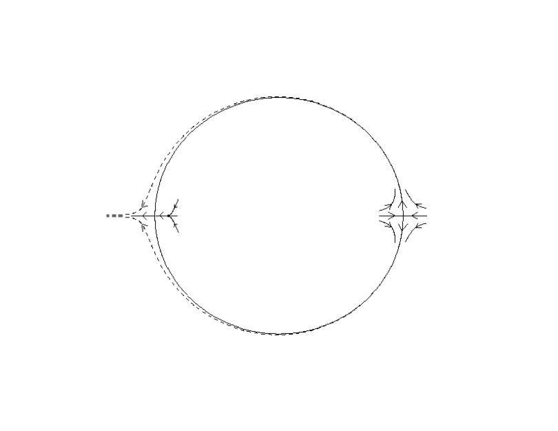
Figure 7.1: Lower Semi-continuity of approximate unstable manifold to the true unstable manifold .

The dashed line in Figure 7.1 represents the flow of the perturbed system ($h>0$); the solid lines represent the unperturbed system ($h=0$). The unstable manifold of the hyperbolic point at $r=1$, $\theta=0$ of the perturbed system now approximates the unstable manifold of the non hyperbolic stationary solution of the unperturbed system as well as the unstable manifold of the unperturbed hyperbolic fixed point. By preparing the above vector field these manifolds remain bounded.

Notice that the unperturbed unstable manifold of the hyperbolic point $r=1$, $\theta=0$ is a proper subset of the perturbed unstable manifold in the limit as $h\rightarrow 0$.

Acknowledgements. The authors are grateful to Edriss Titi for numerous discussions and helpful ideas. The authors would also like to thank Peter Constantin for suggestions on estimating the nonlinear term of the NSE, as well Bernard Minster and Len Margolin for their encouragement and interest. S.S. gratefully acknowledges the support of the Cecil H. and Ida M. Green Foundation and the Institute of Geophysics and Planetary Physics at Scripps Institution of Oceanography. D.A.J. gratefully acknowledges the support of the Institute for Geophysics and Planetary Physics (IGPP) and the Center for Nonlinear Studies (CNLS) at Los Alamos National Laboratory. This work was partially supported by the Department of Energy “Computer Hardware, Advanced Mathematics, Model Physics” (CHAMMP) research program as part of the U.S. Global Change Research Program.

References

- [1] F. Alouges, A. Debussche, On the qualitative behavior of the orbits of a parabolic partial differential equations and its discretization in the neighborhood of a hyperbolic fixed point, Num. Funt. Anal. and Opt., 12, (1991), 253-269.
- [2] F. ALouges, A. Debussche, On the discretization of a partial differential equation in the neighborhood of a periodic orbit, Numer. Math., 65, (1993), 143-175.
- [3] C. Bardos, L. Tartar, Sur l’unicité rétrograde des équations paraboliques et quelques équations voisines, Arch. Rat. Mech. Anal., 50, (1973), 10-25.
- [4] P.W. Bates, K. Lu, and C. Zeng, Existence and persistence of invariant manifolds for semiflows in Banach Space, preprint, (1997).
- [5] D. Beigie, A. Leonard, S. Wiggins, Invariant manifold templates for chaotic advection, Chaos Solitons Frac., 4, (1994), 749-868.
- [6] W.-J. Beyn, On invariant closed curves for one-step methods, Numer. Math., 51, (1987), 103-122.
- [7] W.-J. Beyn, J. Lorenz, Center manifolds of dynamical systems under discretization, Num. Func. Anal. and Opt., 9, (1987), 381–414.
- [8] L. Cattabriga, Su un problema al contorno relativo al sistemo di equazioni di Stokes, Rend. Sem. Mat. Univ. Padova, 31, (1961), 308-340.
- [9] S.-N. Chow, K. Lu, and G.R. Sell, Smoothness of inertial manifolds, J. Math. Anal. Appl., 169, (1992), 283-321.
- [10] P. Constantin, C. Foias, Navier-Stokes Equations, University of Chicago Press, 1988.
- [11] P. Constantin, C. Foias, B. Nicolaenko, R. Temam, Integral Manifolds and Inertial Manifolds for Dissipative Partial differential Equations, Applied Mathematics Sciences, 70, Springer-Verlag, 1988.
- [12] P. Constantin, C. Foias, B. Nicolaenko, R. Temam, Spectral barriers and inertial manifolds for dissipative partial differential equations, J. Dynamics Differential Eqs., 1, (1989), 45-73.
- [13] P. Constantin, C. Foias, R. Temam, On the large time Galerkin approximation of the Navier-Stokes equations, SIAM J. Numer. Anal., 21, (1984), 615-634.
- [14] F. Demengel, J.-M. Ghidaglia, Some remarks on the smoothness of inertial manifolds, Nonlinear Analysis-TMA, 16, (1991), 79-87.
- [15] F. Demengel, J.M. Ghidaglia, Time-discretization and inertial manifolds, Math. Mod. and Num. Anal, 23, (1989), 395-404.
- [16] J. Diéudonne, Foundations of Modern Analysis, Academic Press, New York, 1960.
- [17] D. Ebin and J. Marsden, Groups of diffeomorphisms and the motion of an incompressible fluid, Ann. of Math., 92, (1970), pp. 102-163.
- [18] E. Fabes, M. Luskin, G. Sell, Construction of inertial manifolds by elliptic regularization, J. Diff. Eq., 89, (1991), 355-387.
- [19] N. Fenichel, Persistence and smoothness of invariant manifolds for flows, Ind. Univ. Math. J., 21, (1971), 193-225.
- [20] C. Foias, B. Nicolaenko, G.R. Sell, R. Temam, Inertial manifolds for the Kuramoto-Sivashinsky equation and an estimate of their lowest dimensions, J. Math. Pures Appl., 67, (1988b), 197-226.
- [21] C. Foias, G. Sell, R. Temam, Variétés inertielles des équations différentielles dissipatives, C. R. Acad. Sci. Paris, Sér. I, 301, (1985), 139-142.
- [22] C. Foias, G. Sell, R. Temam, Inertial manifolds for nonlinear evolutionary equations, J. Diff. Eq., 73, (1988), 309-353.
- [23] C. Foias, G. Sell, E.S. Titi, Exponential tracking and approximation of inertial manifolds for dissipative nonlinear equations, J. Dynamics and Diff. Eq., 1, No. 2, (1989), 199-243.
- [24] C. Foias, E.S. Titi, Determining nodes, finite difference schemes and inertial manifolds, Nonlinearity, 4, (1991), 135-153.
- [25] J.K. Hale, Asymptotic Behavior of Dissipative Systems. AMS Mathematical Surveys and Monographs 25, Rhode Island, 1988.
- [26] J.K. Hale, X.-B. Lin, G. Raugel, Upper Semicontinuity of Attractors for Approximations of Semigroups and Partial Differential Equations, Math. Comp., 50, (1988), 89-123.
- [27] D. Henry, Geometric Theory of Semilinear Parabolic Equations. Lecture Notes in Mathematics, Springer-Verlag, New York, 1981.
- [28] J.G. Heywood, R. Rannacher, Finite element approximation of the nonstationary Navier-Stokes problems. Part II Stability of solutions and error estimates uniform in time, SIAM J. Num. Anal., 21, (1986), 615-634.
- [29] A.R. Humphries, Approximation of attractors and invariant sets by Runge-Kutta methods, submitted, (1994).
- [30] M.W. Hirsh, C.C. Pugh, M. Shub, Invariant Manifolds, Lecture Notes in Mathematics, 583, Springer-Verlag, New York, 1977.
- [31] D.A. Jones, On the behavior of attractors under finite difference approximation, Num. Func. Anal. and Opt., 16, (1995), 1155-1180.
- [32] D.A. Jones, E.S. Titi, approximations of inertial manifolds for dissipative nonlinear equations, J. Diff. Eq., 126, (1996).
- [33] D.A. Jones, A.M. Stuart, Attractive invariant manifolds under approximation: inertial manifolds, J. Diff. Eq., 123, (1995), 588-637.
- [34] D.A. Jones, A.M. Stuart, E.S. Titi, Persistence of invariant sets for dissipative evolution equations, Submitted.
- [35] P. Kloeden, J. Lorenz, Stable attracting sets in dynamical systems and their one-step discretizations, SIAM J. Num. Anal., 23, (1986), 986-995.
- [36] S. Lang, Differential and Riemannian Manifolds, Springer-Verlag, New York, 1995.
- [37] S. Larsson, J.M. Sanz-Serna, The behaviour of finite element solutions of semi-linear parabolic problems near stationary points, SIAM J. Numer. Anal., 31, (1994), 1000-1018.
- [38] S. Larsson, J.M. Sanz-Serna, A shadowing result with applications to finite element approximation of reaction-diffusion equations, preprint 1996-05, Dept. of Math. Chalmers Univ. of Tech., Göteborg, Sweden, (1996).
- [39] Y. Li, D.W. McLaughlin, J. Shatah, S. Wiggins, Persistent Homoclinic Orbits for Perturbed Nonlinear Schrödinger Equation, to appear.
- [40] J.L. Lions, Quelques Method de Résolution de Problém aux Limites Non Linéaire, Dunod, Paris, 1969.
- [41] G.J. Lord, Attractors and inertial manifolds for finite difference approximations of the complex Ginzburg-Landau equation, SIAM J. Num Anal., (to appear).
- [42] J. Mallet-Paret, G. Sell, Inertial manifolds for reaction diffusion equations in higher space dimensions, J. Amer. Math. Soc., 1, (1988), 805-866.
- [43] J. Marsden, J. Scheurle, The construction and smoothness of invariant manifolds by the deformation method, SIAM J. Math. Anal., 18, (1987), 1261-1274.
- [44] J. Moser, A rapidly convergent iteration method and non-linear partial differential equations–I, Ann. Scuola Norm. Sup. Pisa, Serie III, XX, (1966), 265-315.
- [45] Y.-R. Ou, S.S. Sritharan, Analysis of regularized Navier-Stokes equations II, Quarterly of Appl. Math., 49, (1991), 687-728.
- [46] A. Pazy, Semigroups of Linear Operators and Applications to Partial Differential Equations, Springer-Verlag, 1983.
- [47] V.A. Pliss, G.R. Sell, Perturbations of attractors of differential equations, J. Differential Eq., 92 (1991), 100-124.
- [48] R. Rosa, R. Temam, Inertial manifolds and normal hyperbolicity. Indiana Univ preprint # 9407.
- [49] R.J. Sacker, A perturbation theorem for invariant manifolds and Hölder continuity, J. Math. Mech., 18, (1969), 705-762.
- [50] G.R. Sell, Y. You, Inertial manifolds: the non-self-adjoint case, J. Diff. Eq., 96, (1992), 203-255.
- [51] V.A. Solonnikov, Estimates of the Green tensor for some boundary problems, Doklady Acad. S.S.S.R., 130, (1960), 988-991, (Russian).
- [52] A.M. Stuart, Perturbation Theory for Infinite-Dimensional Dynamical Systems, Theory and Numerics of Ordinary and Partial Differential Equations, Edited by M. Ainsworth, J. Levesley, W.A. Light, M. Marletta, (1994).
- [53] R. Temam, Navier-Stokes Equations and Nonlinear Functional Analysis, CBMS Regional Conference Series, No. 41, SIAM, Phildelphia, 1983.
- [54] R. Temam, Infinite Dimensional Dynamical Systems in Mechanics and Physics , Springer Verlag, New York, 1988.
- [55] E.S. Titi, On a criterion for locating stable stationary solutions to the Navier-Stokes equations, Nonlinear Anal. TMA, 11, (1987), 1085-1102.
- [56] E.S. Titi, Un critère pour l’approximation des solutions périodiques des équations de Navier–Stokes, C.R. Acad. Sci. Paris, 312, Série I. No. 1, (1991), 41-43.
- [57] I.I. Vorovich, V.I. Yudovich, Stationary flows of incompressible viscous fluids, Mat. Sbornik, 53, (1961), 393-428, (Russian).
- [58] S. Wiggins, Normally hyperbolic invariant manifolds in dynamical systems, Springer-Verlag, New York, 1994.