Orthonormal Compactly Supported Wavelets with Optimal Sobolev Regularity

Abstract: Numerical optimization is used to construct new orthonormal compactly supported wavelets with Sobolev regularity exponent as high as possible among those mother wavelets with a fixed support length and a fixed number of vanishing moments. The increased regularity is obtained by optimizing the locations of the roots the scaling filter has on the interval $(\pi/2,\pi)$. The results improve those obtained by I. Daubechies [Comm. Pure Appl. Math. 41 (1988), 909–996], H. Volkmer [SIAM J. Math. Anal. 26 (1995), 1075–1087], and P. G. Lemarié-Rieusset and E. Zahrouni [Appl. Comput. Harmon. Anal. 5 (1998), 92–105].

AMS Mathematics Subject Classification: 42C15

Keywords: wavelet, regularity, Sobolev exponent

E-mail address: ojanen@math.rutgers.edu

Address: Department of Mathematics - Hill Center; Rutgers, the State University of New Jersey; 110 Frelinghuysen Rd; Piscataway NJ 08854-8019; USA

1 Introduction

To construct orthonormal compactly supported wavelets we use as the starting point the dilation equation

$$\phi(x)=\sqrt{2}\sum_{k\in\mathbb{Z}}c_{k}\phi(2x-k),\qquad x\in\mathbb{R},\qquad c_{k}\in\mathbb{R},$$ (1)

for the scaling function or father function $\phi$. A solution exists in the sense of distributions when $\sum_{k}c_{k}=\sqrt{2}$ and it has compact support if only finitely many of the filter coefficients $c_{k}$ are non-zero (in fact, if $c_{k}\not=0$ only for $k\in\{0,\dots,n\}$ then the support of $\phi$ is contained in $[0,n]$). The solution of the dilation equation is given by

$$\widehat{\phi}(\xi)=\prod_{j=1}^{\infty}m_{0}(2^{-j}\xi),$$ (2)

where the trigonometric polynomial $m_{0}(\xi)$ is the scaling filter of $\phi$,

$$m_{0}(\xi)=\frac{1}{\sqrt{2}}\sum_{k\in\mathbb{Z}}c_{k}e^{-ik\xi}.$$ (3)

The condition when the solution to (1) yields wavelets can be expressed in terms of the scaling filter $m_{0}(\xi)$. If $m_{0}$ satisfies

$$\lvert m_{0}(\xi)\rvert^{2}+\lvert m_{0}(\pi+\xi)\rvert^{2}=1,\qquad\xi\in\mathbb{R},$$ (4)

$m_{0}(0)=1$, and a technical condition called the Cohen criterion holds, then there exists a scaling function and wavelet pair [1], [4, Section 6.3]. We will not need exact details about Cohen’s condition, we only use that if $m_{0}$ does not vanish on $[-\pi/2,\pi/2]$, then it satisfies the criterion.

If $\phi$ is such that it gives rise to a wavelet, the wavelet $\psi$ is obtained by

$$\psi(x)=\sum_{k\in\mathbb{Z}}(-1)^{k}c_{1-k}\phi(2x-k).$$

Note that then $\phi$ and $\psi$ have the same regularity properties.

The original construction of orthonormal compactly supported wavelets by I. Daubechies [3] considers a trigonometric polynomial $m_{0}$ with at most $2N$ non-zero coefficients $c_{0}$, …, $c_{2N-1}$. The polynomial $m_{0}$ is required to satisfy (4) and to have a zero at $\pi$ of maximal order $N$ (the order of the zero is also the number of vanishing moments the corresponding wavelet has). The resulting equations can be solved and the constructed $m_{0}$ has no roots on $(-\pi,\pi)$, hence it satisfies the Cohen criterion. ([4] is a comprehensive reference for these results.)

To construct smoother wavelets our approach is to reduce the order of the zero $m_{0}$ has at $\pi$ and instead to introduce zeros on the interval $(\pi/2,\pi)$. Keeping $N$ and the number of zeros on $(\pi/2,\pi)$ fixed we use numerical optimization to choose the locations of the roots so that the resulting wavelets are as smooth as possible. We are able to construct wavelets that are more regular than those introduced in [3], [8], and [15].

This paper is organized as follows: in Section 2 we state our results and compare them to the above mentioned papers. The methods used are described in Section 3, and in Section 4 the optimization is discussed in detail. We comment in Section 5 on some other approaches that were tried. Finally, filter coefficients for selected most regular wavelets are listed in section 6.

2 Results

In the numerical optimization for smoothness we studied wavelets with up to $40$ filter coefficients and whose scaling filter has up to four roots on the interval $(\pi/2,\pi)$. The Sobolev regularity exponents of the most regular wavelets found are shown in Table 1. (By the Sobolev regularity exponent $s_{0}$ of $\phi$ we mean $s_{0}=\sup\{s\colon\phi\in H^{s}\}$, where $H^{s}$ is the Sobolev space consisting of all $f\in L^{2}(\mathbb{R})$ such that $(1+\lvert\xi\rvert^{2})^{s/2}\widehat{f}(\xi)\in L^{2}(\mathbb{R})$.) The results are also summarized in Figure 1.

		Sobolev regularity exponent $s_{0}$
$2N$		${n_{z}}=0$	${n_{z}}=1$	${n_{z}}=2$	${n_{z}}=3$	${n_{z}}=4$
2		0.50
4		1.00
6		1.42	1.00
8		1.78	1.82
10		2.10	2.26	1.00
12		2.39	2.66	2.00
14		2.66	3.02	3.00	1.00
16		2.91	3.37	3.48	2.00
18		3.16	3.72	3.92	3.00	1.00
20		3.40	4.07	4.32	4.00	2.00
22		3.64	4.42	4.73	4.76	3.00
24		3.87	4.78	5.14	5.22	4.00
26		4.11	5.14	5.55	5.67	5.00
28		4.34	5.50	5.95	6.10	5.84
30		4.57	5.85	6.34	6.51	6.38
32		4.79	6.19	6.71	6.89	6.88
34		5.02	6.52	7.09	7.25	7.30
36		5.24	6.83	7.45	7.62	7.69
38		5.47	7.15	7.81	7.99	8.08
40		5.69	7.46	8.17	8.37	8.51

Table 1: The best Sobolev regularity exponents found. The length of the filter is $2N$ and the filter $m_{0}$ has $n_{z}$ roots on the interval $(\pi/2,\pi)$. For comparison the column ${n_{z}}=0$ gives the Sobolev exponents of the Daubechies wavelets [3], the other columns are new.

The column ${n_{z}}=0$ gives the Sobolev exponents for the Daubechies wavelets constructed in [3]. For $N\geq 4$ we have constructed wavelets which are more regular. For large values of $N$ there are four families of wavelets corresponding to different numbers of roots on $(\pi/2,\pi)$, and the regularity increases with the number of roots.

To relate these results to Hölder regularity, it can be shown that the Hölder regularity exponent $\alpha_{0}=\sup\{\alpha\colon\phi\in C^{\alpha}\}$ satisfies $\alpha_{0}\in[s_{0}-1/2,s_{0}]$ [13, Corollary 9.9]. Here $C^{\alpha}$ consists of functions that are continuously differentiable up to order equal to the integer part of $\alpha$, and the highest order continuous derivative belongs to the (standard) Hölder class with exponent equal to the fractional part of $\alpha$.

Note that in each column ${n_{z}}=1$, …$4$, the first few entries are smaller than in the previous columns on the same row. This is not surprising, since it can be shown that in order to have $\psi\in H^{n}$, the wavelet $\psi$ must have at least $n+1$ vanishing moments [13, Proposition 8.3]. The wavelets corresponding to the entries in the table have $N-2{n_{z}}$ vanishing moments.

We show below (see Section 4.2) that the entries in the column ${{n_{z}}=1}$ are best possible in the sense that the corresponding wavelets are smoothest possible among those with $2N\geq 8$ coefficients and at least $N-2$ vanishing moments.

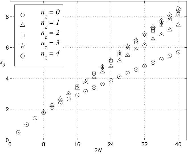
Figure 1: The Sobolev regularity exponents $s_{0}$ from Table 1. For clarity only those are shown that are better than the ones with the same length filter but with fewer roots on $(\pi/2,\pi)$.

For higher values of ${n_{z}}$ the exponents listed in Table 1 are best possible among those wavelets with $2N$ coefficients and whose scaling filter $m_{0}$ has the indicated number of zeros on $(\pi/2,\pi)$. Some of these were subjected to extensive tests by choosing many different initial approximations for the optimizer. Note also how the results, except for the first few entries, lie on almost straight lines in Figure 1. See also Figures 3 and 7 which show typical examples of the regularity exponent as a function of the location of the roots.

However, it is not completely clear if the results for $n_{z}\geq 2$ are best possible if we consider wavelets with the same number of vanishing moments as above but do not insist on $m_{0}$ having roots on $(\pi/2,\pi)$. We come back to this at the end of Section 4.3.

We remark that the case $2N=10$, ${n_{z}}=1$ appears already in [10].

More regular wavelets than the original Daubechies family have been constructed by I. Daubechies [5], H. Volkmer [15], P. G. Lemarié-Rieusset and E. Zahrouni [8]. We discuss the wavelets from [5] in Section 4.1.

H. Volkmer [15] computes only the asymptotic regularity ratio $\lim_{N\rightarrow\infty}\sigma/2N$ and constructs wavelets for which the ratio is close to $0.19$. Note that for many entries in Table 1 the ratio $\sigma/2N$ is over $0.21$.

P. G. Lemarié-Rieusset and E. Zahrouni [8] discuss what they call the Matzinger wavelets: the scaling filter has a multiple root at $2\pi/3$ and no other roots on $(\pi/2,\pi)$. Our results are better, e.g., the smoothest one they construct has $34$ coefficients and Sobolev exponent $6.13$. Table 1 shows that already with ${n_{z}}=1$ our wavelet with the same number of coefficients is more regular. In fact, for each value of $N$ the ${n_{z}}=1$ wavelet listed in Table 1 is better than the smoothest wavelet discussed in [8].

3 Methods

We begin by describing the theorem that allows us to compute exactly the Sobolev regularity exponent of solutions to (1). Define another trigonometric polynomial, $r(\xi)$, by factoring out all zeros of $\lvert m_{0}(\xi)\rvert^{2}$ at $\xi=\pi$, that is, let

$$\lvert m_{0}(\xi)\rvert^{2}=\left(\frac{1+\cos\xi}{2}\right)^{M}r(\xi),$$ (5)

where $M\in\mathbb{N}$ is chosen so that $r(\pi)\not=0$. The function $r$ is used to define an operator on $C[0,\pi]$ by

$$T_{r}u(\xi)=r(\xi/2)u(\xi/2)+r(\pi-\xi/2)u(\pi-\xi/2).$$ (6)

The Sobolev regularity exponent of a solution to the dilation equation (1) is given by the following theorem, proved independently by L. Villemoes and T. Eirola:

Theorem 3.1 ([7, 13])

Suppose $\phi$ is a solution to (1), $M$, $r$, and $T_{r}$ are as above, and $r$ satisfies the Cohen criterion. Then $\phi\in H^{s}$ if and only if $s<s_{0}=M-\log_{4}\rho(T_{r})$, where $\rho(T_{r})$ is the spectral radius of $T_{r}$ on $C[0,\pi]$.

If $r$ is a polynomial of cosines of degree at most $d$, i.e., $r(\xi)=\sum_{k=0}^{d}b_{k}\cos(k\xi)$, then $T_{r}$ maps the space spanned by $\{\cos(k\xi)\}_{k=0}^{d}$ into itself and the spectral radius of $T_{r}$ can be calculated from the eigenvalues of a finite matrix [7, 13].

Suppose we want to look at a filter of length $2N$ (i.e., a filter $m_{0}$ with at most $2N$ non-zero coefficients), such that $m_{0}$ has a zero of order $M$ at $\pi$ and ${n_{z}}$ zeros on the interval $(\pi/2,\pi)$. Note that $M$ is also the number of vanishing moments the associated wavelet has (if it exists).

Define a new sequence of coefficients by

$$\lvert m_{0}(\xi)\rvert^{2}=\sum_{k=0}^{2N-1}a_{k}\cos(k\xi).$$ (7)

The orthonormality condition (4) is equivalent to

$$a_{0}=\frac{1}{2},\qquad a_{2k}=0,\quad\text{for $k=1$, \ldots, $N-1$.}$$

We first use the zero of $m_{0}$ at $\pi$ to find (linear) relations among the $\{a_{k}\}$: we express $a_{k}$, $k=1$, $3$, …, $2M-1$, in terms of $a_{k}$, $k=2M+1$, $2M+3$, …, $2N-1$. Note that there are $N-M=2n_{z}$ independent parameters. For convenience we switch to a new set of parameters $\mathbf{v}=(v_{1},\dots,v_{n_{z}})$ that are simply obtained from $a_{k}$, $k=2M+1$, $2M+3$, …, $2N-1$ by scaling the latter so that $\mathbf{v}=(1,\dots,1)$ corresponds to the Daubechies wavelets (i.e., all roots of $m_{0}$ are at $\pi$). The function $r$ is then obtained by factoring $\big{(}(1+\cos\xi)/2\big{)}^{M}$ from $\lvert m_{0}(\xi)\rvert^{2}$. (The computations are done quickly with a symbolic algebra system such as Mathematica by using the Taylor polynomial of $m_{0}$ at $\pi$.)

When $r$ has low degree it is easy to compute the matrix of the operator $T_{r}$ on the span of $\{\cos(k\xi)\}_{k=0}^{\deg r}$ algebraically—an example is done in Section 4.1. When the degree is high it is more convenient to compute the matrix numerically by using the fast Fourier transform. Finally, $s_{0}$ is computed from the largest eigenvalue of this matrix.

Note that fixing the value of $\mathbf{v}$ does not uniquely determine the wavelet, since it only determines the absolute value of $m_{0}(\xi)$. For our purposes this is enough, since all those wavelets have the same regularity by Theorem 3.1.

4 Optimization

4.1 One degree of freedom

First consider wavelets with four filter coefficients, i.e., $N=2$, and one vanishing moment. Then

$$\lvert m_{0}(\xi)\rvert^{2}=\frac{1}{2}+a_{1}\cos\xi+a_{3}\cos 3\xi$$

and $m(\pi)=0$ gives $a_{1}=1/2-a_{3}$. To compute $r$ we get

$$\lvert m_{0}(\xi)\rvert^{2}=\frac{1}{2}(1+\cos\xi)(8a_{3}\cos^{2}\xi-8a_{3}\cos\xi+1)=\frac{1}{2}(1+\cos\xi)r(\xi).$$

The Daubechies wavelet has two vanishing moments, hence $r(\pi)=0$, which implies $a_{3}=-1/16$. Introduce the new parameter $v$ by $a_{3}=-v/16$. Then

$$r(\xi)=-\frac{v}{2}\cos^{2}\xi+\frac{v}{2}\cos\xi+1,$$

and the matrix of the operator $T_{r}$ on the span of $\{1,\cos\xi,\cos 2\xi\}$ is easily computed to be

$$\frac{1}{4}\begin{pmatrix}8-2v&-2v&0\\ 2v&2v&0\\ -v&8-2v&-v\end{pmatrix}.$$

The eigenvalues of this matrix are

$$\lambda_{1}=1+\sqrt{1-v},\quad\lambda_{2}=1-\sqrt{1-v},\quad\text{and}\quad\lambda_{3}=-\frac{v}{4}.$$

Recall that $r(\xi)$ has to be non-negative. In particular $r(\pi)\geq 0$ gives $v\leq 1$. Then $\lambda_{1}\geq 1$ and $\rho(T_{r})\geq 1$ and so $s_{0}\leq 1$ for all admissible values of $v$. The Daubechies wavelet corresponds to $v=1$ and $s_{0}=1$, for all other wavelets in this family we have $v<1$, and therefore $s_{0}<1$.

Numerical results show this is also the case for wavelets with larger values of $N$ and with one degree of freedom. Thus the original Daubechies [3] wavelets are the smoothest possible among wavelets with $2N$ coefficients and at least $N-1$ vanishing moments.

I. Daubechies [5] has also constructed wavelets that have higher Hölder regularity exponents than the ones originally constructed in [3]. In [5] the cases $2N=4$ and $2N=6$ were studied. Table 2 gives both Hölder and Sobolev exponents for two wavelets from the original construction in [3]. (The Sobolev exponents are as in Table 1, the Hölder exponents are from [6].) Table 3 gives the exponents for the two wavelets constructed in [5]. The Sobolev exponents for the new wavelets are easily computed from Theorem 3.1, e.g., for $2N=4$ we get $s_{0}=\log_{4}(10/3)\approx 0.87$.

Comparing the numbers in Tables 2 and 3 an interesting phenomenon appears: both for $2N=4$ and for $2N=6$ we have an example of two functions, one of which is slightly more regular when regularity is measured in the Hölder sense, but the opposite is true if Sobolev regularity is used.

$2N$		Hölder	Sobolev
4		0.55	1.00
6		1.09	1.42

Table 2: Hölder and Sobolev regularity exponents for the wavelets constructed in [3].

$2N$		Hölder	Sobolev
4		0.59	0.87
6		1.40	1.31

Table 3: Hölder and Sobolev regularity exponents for the Hölder smoothest wavelets constructed in [5]. (The Hölder exponents are lower bounds for the actual value.)

4.2 Two degrees of freedom

Optimization was done on the $\mathbf{v}=(v_{1},v_{2})$ parameters. Since some values of $\mathbf{v}$ yield an $r_{\mathbf{v}}$ that takes on also negative values, this is now a constrained optimization problem with the nonlinear constraint $\min_{0\leq\xi\leq\pi}r_{\mathbf{v}}(\xi)\geq 0$.

Figure 2 shows a plot of the Sobolev exponent as a function of the parameters $v_{1}$, $v_{2}$. A typical example of the exponent on the boundary of the feasible region is given in Figure 3, where the exponent is plotted as a function of the double root that $r$ has on $(\pi/2,\pi)$. Figure 4 shows a plot of $r(\xi)$ and $\lvert m_{0}(\xi)\rvert$ for the optimal choice of the root. Note that the Cohen criterion is clearly satisfied.

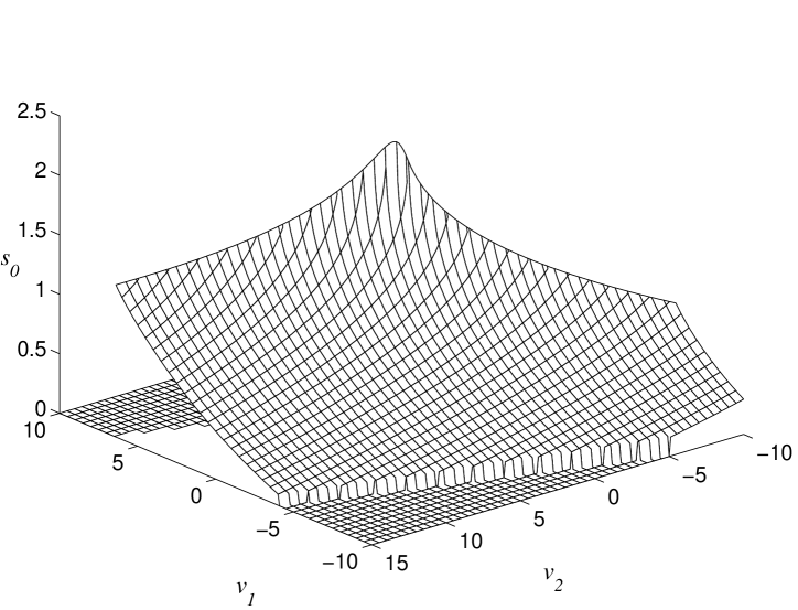
Figure 2: The Sobolev regularity exponent $s_{0}$ as a function of the parameters $\mathbf{v}=(v_{1},v_{2})$ for the case $2N=10$. (When $\mathbf{v}$ is outside the admissible region $\min r_{\mathbf{v}}\geq 0$ we plot $s_{0}$ as zero.)

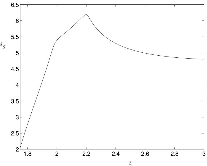
Figure 3: The Sobolev regularity exponent $s_{0}$ as a function of the root $z$ that $m_{0}$ and $r$ have on the interval $(\pi/2,\pi)$. Here $2N=32$, ${n_{z}}=1$.

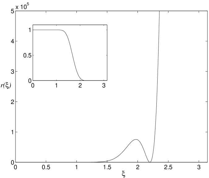
Figure 4: The function $r(\xi)$ for $2N=32$, ${n_{z}}=1$ corresponding to optimal regularity. The inset shows the graph of $\lvert m_{0}(\xi)\rvert$.

Numerical optimization of the regularity exponent was done by using the Matlab Optimization Toolbox. The smoothest wavelet was always found on the boundary of the feasible region $\{\mathbf{v}\in\mathbb{R}^{2}\colon\min r_{\mathbf{v}}\geq 0\}$, that is, the optimal $r$ has a double root on $(\pi/2,\pi)$. For comparison with the Daubechies family, the most regular scaling function with ten coefficients is shown in Figure 5 together with its first derivative and graphs of the corresponding Daubechies scaling function. Figure 6 shows graphs of the Fourier transforms of the scaling functions.

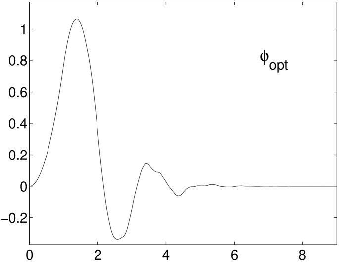
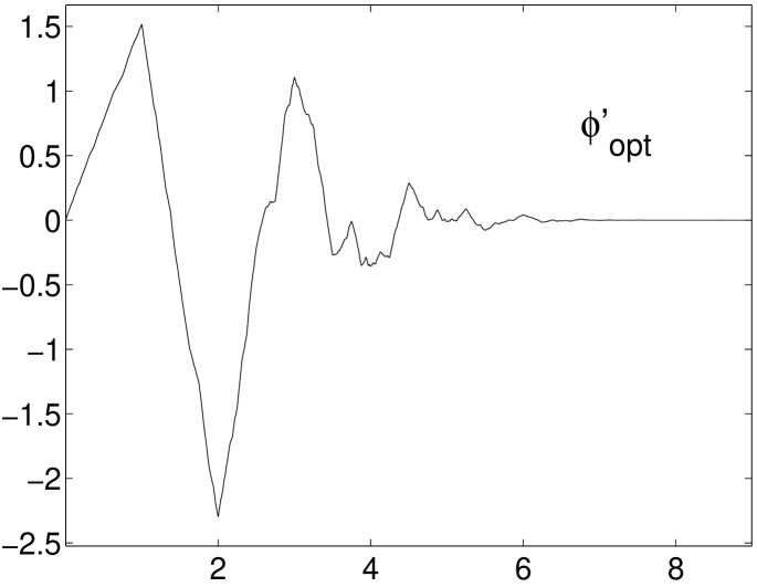
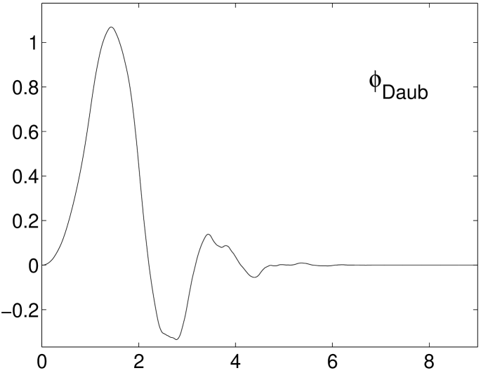
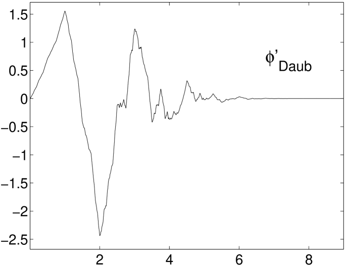
Figure 5: On the top the most regular scaling function and its first derivative, on the bottom the Daubechies scaling function and its first derivative. Here $2N=10$.

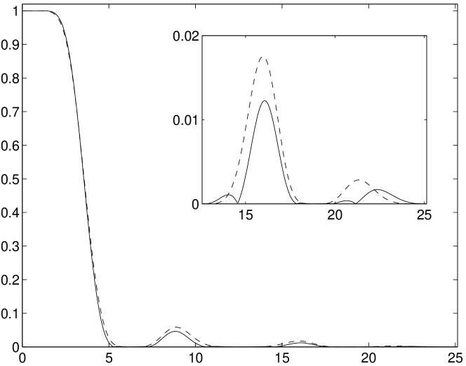
Figure 6: Graphs of $\widehat{\phi}(\xi)$ given by (2) for the most regular (solid curve) and Daubechies wavelets (dashed) with ten coefficients. The blow-up of the interval $[4\pi,8\pi]$ in the inset shows how the root of $m_{0}$ on $(\pi/2,\pi)$ improves decay of $\widehat{\phi}$, hence regularity of $\phi$.

Table 4 lists the locations of the root of $m_{0}$ on $(\pi/2,\pi)$ for the most regular wavelets.

$2N$		$z$			$2N$		$z$
8		2.	8762		26		2.	2346
10		2.	6450		28		2.	2213
12		2.	5099		30		2.	2099
14		2.	4200		32		2.	1995
16		2.	3630		34		2.	1894
18		2.	3238		36		2.	1799
20		2.	2939		38		2.	1712
22		2.	2701		40		2.	1633
24		2.	2506

Table 4: Location of the root of $r$ for the most regular wavelets for ${n_{z}}=1$.

The set $\{\mathbf{v}\in\mathbb{R}^{2}\colon\min r_{\mathbf{v}}\geq 0\}$ contains a parametrization of all wavelets with $2N$ coefficients and $N-2$ vanishing moments. Together with the results of the previous section this shows the regularity exponents in the ${n_{z}}=1$ column of Table 1 are the best possible among wavelets with at least $N-2$ vanishing moments and $2N\geq 8$ filter coefficients.

4.3 More degrees of freedom

The approach of the previous section did not work with higher degrees of freedom, i.e., with $\mathbf{v}\in\mathbb{R}^{n}$, $n\geq 3$, due to convergence problems with Matlab’s constrained optimizer (since $r$ is a polynomial of high degree, problems with the constraint $\min r_{\mathbf{v}}\geq 0$ are not unexpected). Instead, the optimization was done by considering the Sobolev regularity exponent $s_{0}$ as a function of the zeros $\mathbf{z}=(z_{1},\dots,z_{n_{z}})$ of $r$ on $(\pi/2,\pi)$. The benefits are that now we are studying an unconstrained optimization problem and the number of degrees of freedom is halved.

For a fixed value of $\mathbf{z}$ we can solve for the parameters $\mathbf{v}$ discussed above by requiring $r_{\mathbf{v}}(\mathbf{z})=r^{\prime}_{\mathbf{v}}(\mathbf{z})=0$. This is a linear system, though it may be badly conditioned when $r$ is of high degree. (This problem was overcome by using Mathematica and 30 digit precision in the computations.)

The optimal locations for the roots of $m_{0}$ are given in Tables 5, 6, and 7. Figure 7 shows a typical example of the regularity exponent as a function of the roots and Figure 8 shows a plot of $r(\xi)$ for the optimal choice of the roots. Again the Cohen criterion is clearly satisfied.

As discussed in Section 2 it is still open what happens if $r$ is not required to have as many roots on $(\pi/2,\pi)$ as above. Recall that $r$ is essentially a polynomial (of cosines) of high degree. Figure 8 shows high peaks between the roots of $r$. Is it possible to make these peaks lower by not requiring $r$ to vanish between them? However, even if this were the case, it is not clear how the regularity exponent would change.

$2N$		$z_{1}$			$z_{2}$
16		2.	3525		2.	8336
18		2.	3150		2.	7491
20		2.	2790		2.	7110
22		2.	2496		2.	6867
24		2.	2260		2.	6691
26		2.	2072		2.	6566
28		2.	1931		2.	6448
30		2.	1814		2.	6337
32		2.	1718		2.	6255
34		2.	1630		2.	6217
36		2.	1557		2.	6199
38		2.	1501		2.	6192
40		2.	1450		2.	6186

Table 5: Location of the roots of $r$ for the most regular wavelets for ${n_{z}}=2$.

$2N$		$z_{1}$			$z_{2}$			$z_{3}$
22		2.	2474		2.	6807		3.	0380
24		2.	2199		2.	6571		2.	9637
26		2.	2005		2.	6413		2.	9197
28		2.	1871		2.	6303		2.	8892
30		2.	1761		2.	6229		2.	8710
32		2.	1668		2.	6196		2.	8598
34		2.	1582		2.	6184		2.	8440
36		2.	1497		2.	6172		2.	8071
38		2.	1425		2.	6143		2.	7488
40		2.	1369		2.	6174		2.	7109

Table 6: Location of the roots of $r$ for the most regular wavelets for ${n_{z}}=3$.

$2N$		$z_{1}$			$z_{2}$			$z_{3}$			$z_{4}$
28		2.	2307		2.	4928		2.	9401		3.	0099
30		2.	1767		2.	6544		2.	6958		3.	0326
32		2.	1657		2.	6250		2.	8334		2.	9133
34		2.	1581		2.	5655		2.	6837		2.	9097
36		2.	1480		2.	5568		2.	6178		2.	9207
38		2.	1362		2.	4881		2.	6498		2.	9159
40		2.	1316		2.	6311		2.	7035		2.	8414

Table 7: Location of the roots of $r$ for the most regular wavelets for ${n_{z}}=4$.

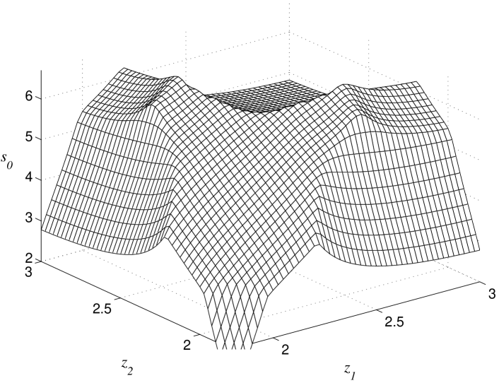
Figure 7: The Sobolev regularity exponent $s_{0}$ as a function of the roots $z_{1}$, $z_{2}$ that $m_{0}$ and $r$ have on the interval $(\pi/2,\pi)$. Here $2N=32$.

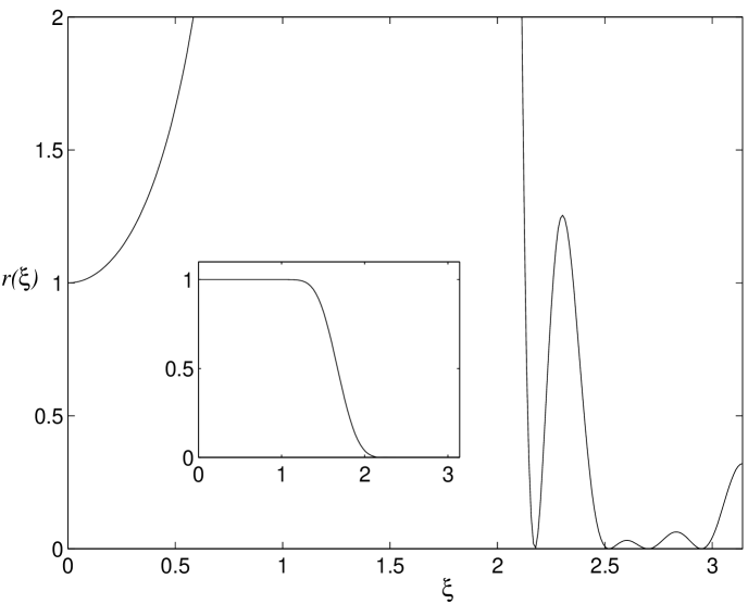
Figure 8: The function $r(\xi)$ for $2N=32$, ${n_{z}}=4$ corresponding to optimal regularity. The inset shows the graph of $\lvert m_{0}(\xi)\rvert$.

5 Other parametrizations

The parametrization of the wavelets could also be based on the original result of Daubechies [4, Proposition 6.1.2], or on a similar result by Wells [16]. Both of these were tried, but they suffer from the same difficulty as our parametrization in terms of the vector $\mathbf{v}$: there is a non-linear constraint that makes numerical optimization for complicated filters impossible with the software that was used. (These parametrizations could be used as the starting point for a parametrization in terms of roots of $m_{0}$, though.)

Direct parametrizations of the coefficients $c_{k}$ have been introduced in [9, 11, 12, 17], but in contrast to our approach the moment condition (5) is then a system of non-linear equations of the parameters (see in particular [17, Theorem 2]). For wavelets with $2N$ filter coefficients and $M$ vanishing moments there are $N$ parameters and $M-1$ non-linear equations. The equations can be used to solve for $M-1$ of the parameters when the rest are kept fixed. Numerical experiments show, however, that typically there are multiple solutions that correspond to wavelets with different regularity, making this approach unsuitable for optimizing regularity. Moreover, these parametrizations provide an expression directly for $m_{0}(\xi)$, but for the computation of the regularity exponent we need $r(\xi)$.

Only the parametrization in terms of the roots of $m_{0}$ has provided the computational simplicity necessary for optimizing regularity when the filter is complicated: recall that there are only linear equations to be solved.

6 Filter coefficients

The optimization provides us with an expression for $\lvert m_{0}(\xi)\rvert$. The (low-pass) filter coefficients $c_{k}$ in (1) are then easy to compute by using spectral factorization [4, p. 172]. The coefficients for selected most regular wavelets are listed in Tables 8–10. To guarantee that $m_{0}$ satisfies the orthonormality condition (4) to high precision, the factorization was done with Mathematica using 30 digit precision and checked by repeating the computations with 60 digit precision: the results are accurate to the number of decimals given in the tables.

$c_{k}$
1.	807084186243315e-1
6.	272955371644549e-1
7.	021176047824324e-1
1.	120128480002895e-1
-2.	446469866533168e-1
-2.	970511286791226e-2
8.	518480911807988e-2
-7.	179751673520435e-3
-1.	625706468497944e-2
4.	683260563235789e-3

Table 8: $2N=10$, ${n_{z}}=1$

$c_{k}$
4.	409469394058257e-2
2.	599093138855805e-1
6.	057694016921036e-1
6.	371421499968423e-1
1.	364367462665367e-1
-2.	883826797756209e-1
-1.	270531514862528e-1
1.	555314597190144e-1
6.	802158361295070e-2
-8.	862450100620332e-2
-2.	399047021783915e-2
4.	548910378211001e-2
2.	025062066984338e-3
-1.	790050908684461e-2
3.	315675665790194e-3
4.	335970768455452e-3
-1.	852310988320677e-3
-3.	359209223085526e-4
3.	395506340120817e-4
-5.	760617447778257e-5

Table 9: $2N=20$, ${n_{z}}=2$

$c_{k}$
9.	286962261105670e-3
8.	065009178408755e-2
2.	975638977797063e-1
5.	849583107003815e-1
5.	940950288790657e-1
1.	464131039850201e-1
-2.	899897992799635e-1
-1.	888671876256031e-1
1.	529318071875427e-1
1.	393659002859078e-1
-9.	487951734281382e-2
-8.	688845136891955e-2
6.	416864747737246e-2
4.	586586496411027e-2
-4.	242829324588881e-2
-1.	870129886474555e-2
2.	492219541071851e-2
4.	323699937678751e-3
-1.	195215551785778e-2
7.	996165686836154e-4
4.	259303332169016e-3
-1.	263090636020650e-3
-9.	623632092949613e-4
5.	655466161125865e-4
7.	527472879191102e-5
-1.	260995097154413e-4
2.	020452355886283e-5
1.	026632536894423e-5
-4.	411797664714925e-6
5.	080242007105260e-7

Table 10: $2N=30$, ${n_{z}}=3$

7 Conclusions

We have constructed wavelets that are more regular than any of the wavelets that have appeared in the literature with the same number of filter coefficients, thus improving the ratio of regularity to complexity. Our methods show that a numerical optimization approach provides the flexibility necessary to construct highly regular wavelets while keeping the number of vanishing moments of the wavelet as high as possible.

We have also shown our results are optimal for wavelets with $2N$ filter coefficients and at least $N-2$ vanishing moments.

References

- [1] A. Cohen, Ondelettes, analyses multirésolutions et filtres miroirs en quadrature, Ann. Inst. H. Poincaré Anal. Non Linéaire 7 (1990), no. 5, 439–459.
- [2] A. Cohen and J.-P. Conze, Régularité des bases d’ondelettes et mesures ergodiques, Rev. Mat. Iberoamericana 8 (1992), no. 3, 351–365.
- [3] I. Daubechies, Orthonormal bases of compactly supported wavelets, Comm. Pure Appl. Math. 41 (1988), 909–996.
- [4] , Ten Lectures on Wavelets, Society for Industrial and Appl. Math., 1992.
- [5] , Orthonormal bases of compactly supported wavelets II. Variations on a theme, SIAM J. Math. Anal. 24 (1993), no. 2, 499–519.
- [6] I. Daubechies and J. C. Lagarias, Two-scale difference equations. II. Local regularity, infinite products of matrices and fractals, SIAM J. Math. Anal. 23 (1992), no. 4, 1031–1079.
- [7] T. Eirola, Sobolev characterization of solutions of dilation equations, SIAM J. Math. Anal. 23 (1992), no. 4, 1015–1030.
- [8] P. G. Lemarié-Rieusset and E. Zahrouni, More regular wavelets, Appl. Comput. Harmon. Anal. 5 (1998), 92–105.
- [9] J.-M. Lina and M. Mayrand, Parametrizations for Daubechies wavelets, Phys. Rev. E (3) 48 (1993), no. 6, R4160–R4163.
- [10] H. Ojanen, Remarks on the Sobolev regularity of wavelets and interpolation schemes, Research Reports A305, Helsinki Univ. of Technology, Inst. of Math., 1991.
- [11] D. Pollen, for a subfield of , J. Amer. Math. Soc. 3 (1990), no. 3, 611–624.
- [12] J. Schneid and S. Pittner, On the parametrization of the coefficients of dilation equations for compactly supported wavelets, Computing 51 (1993), no. 2, 165–173.
- [13] L. F. Villemoes, Energy moments in time and frequency for two-scale difference equation solutions and wavelets, SIAM J. Math. Anal. 23 (1992), no. 6, 1519–1543.
- [14] H. Volkmer, On the regularity of wavelets, IEEE Trans. Inform. Theory 38 (1992), no. 2, part 2, 872–876.
- [15] , Asymptotic regularity of compactly supported wavelets, SIAM J. Math. Anal. 26 (1995), no. 4, 1075–1087.
- [16] Wells, R. O., Jr., Parametrizing smooth compactly supported wavelets, Trans. Amer. Math. Soc. 338 (1993), no. 2, 919–931.
- [17] H. Zou and A. H. Tewfik, Parametrization of compactly supported orthonormal wavelets, IEEE Trans. Signal Processing 41 (1993), no. 3, 1428–1431.