Algorithms for recognizing knots and 3-manifolds

1 Algorithms and Classifications.

Algorithms are of interest to geometric topologists for two reasons. First, they have bearing on the decidability of a problem. Certain topological questions, such as finding a classification of four dimensional manifolds, admit no solution. It is important to know if other problems fall into this category. Secondly, the discovery of a reasonably efficient algorithm can lead to a computer program which can be used to examine interesting examples. In this paper we will survey some topological algorithms, in particular those that relate to distinguishing knots. Our approach is somewhat informal, with many details omitted, but references are given to sources which develop these ideas in full depth.

Given a question $Q$, a decision procedure for $Q$ or an algorithm to decide $Q$ can be thought of as a computer program which will produce an answer to $Q$ in a finite amount of time. A formal description of an algorithm or a computer is given by the notion of a Turing machine. A Turing machine is a basic computational device that reads and writes onto a tape. The questions such a machine can decide are the same as those that can be decided by more complicated computers. The tape is divided into cells, which the Turing machine can read from and write to, one at a time. The tape has a leftmost cell, but is infinite to the right. A finite set of symbols can be written onto the tape - the usual English alphabet if we wish. The Turing machine has a finite number of possible states, and its behavior is determined by its state. Initially, some finite number of cells on the tape contain symbols and the rest are blank. At each time interval, the Turing machine scans the symbol at the current tape location, and in a manner determined by the symbol and its current state it: 1. Changes to a new state. 2. Overwrites the symbol it has read with a new symbol. 3. Moves the tape one cell left or right. Some states are final. The computation ends when they occur.

$Q$ is called recursive if there is an algorithm that produces an answer in a finite amount of time. Showing that there is an algorithm to decide $Q$ is equivalent to showing that $Q$ is recursive. It is often easier to find an algorithm that takes a finite amount of time to give a “Yes” answer to a question, but may run forever if the answer is “No”. This does not establish that the question is recursive. A rather different issue is the amount of time it takes an algorithm to answer a given question. This is determined by its computational complexity. Computational complexity is a measure of the difficulty of a problem, and can have implications to a real world implementation of an algorithm, but is independent of the decidability of a question. A good reference for the notions of Turing machine, algorithms and decidability is [8].

There are natural questions that do not admit any algorithm to decide them. A famous example is the word problem for finitely presented groups. Given a group described by a collection of generators and relations

$$G=\{x_{1},\dots,x_{m};r_{1},\dots,r_{n}\},$$

this question asks whether a given product of generators represents the identity element. It was shown by Novikov and Boone that there are groups in which there is no algorithm to decide this question. An exposition can be found in [20]. Closely related is the question of whether a finitely presented group $G$ is isomorphic to the trivial group, which also cannot be decided by an algorithm. Note however that it is easy to construct an algorithm which will answer the triviality question with a “Yes” in finite time if the group is trivial. An algorithm which constructs all products of relations and their inverses and checks for the generators in this list will accomplish this goal. However this algorithm will run on forever if the group is non-trivial, so it does not decide the triviality question.

The notion of a classification is closely related. Define a classification of a set of objects to be a list containing each element of the set once. Finding a classification of some set of objects does not necessarily end its mathematical interest. As an example, it is easy to classify the natural numbers.

I am indebted to W. Jaco and G. Kuperberg for helpful discussions.

2 Topological algorithms

We will now consider the problem of classifying compact orientable 3-manifolds. We seek a list containing each 3-manifold once, with the property that if we are given a 3-manifold in some standard form then we can determine where on the list it appears.

While surfaces have been classified for some time, a classification remains elusive for 3-manifolds. Markov showed that the Novikov-Boone results implied that the classification problem for 4-manifolds was not solvable [15]. Given a finitely presented group, a compact 4-manifold (or $n$-manifold with $n>4$) can be constructed with that group as its fundamental group. Markov showed that a classification of 4-manifolds could be used to give an algorithm to solve the problem of whether this presentation defines the trivial group, which we have seen is impossible. While it seems unlikely that a similar type of problem arises for 3-manifolds, it is still unknown whether they can be classified.

Here is an example of something that is not a classification of 3-manifolds. All closed 3-manifolds can be triangulated [16]. Since there are only finitely many ways to glue together $k$ tetrahedra, we can construct all of these systematically. A resulting complex is a manifold exactly when the links of all vertices are 2-spheres, a condition that is easy to check. Throwing away the non-manifolds gives a method of generating a list containing all 3-manifolds. The drawback is that a given manifold appears many times in this list, and there is no known method to decide whether two manifolds in this list are homeomorphic. However this procedure would lead to a classification if we could solve the
Recognition Problem for 3-manifolds: Give an algorithm to decide whether two closed 3-manifolds are homeomorphic.

The 3-manifolds are specified by the finite amount of data needed to describe a finite triangulation. This data can be extracted from any of the standard ways of describing 3-manifolds, such as surgery on a link, Heegaard diagrams, hierarchies, etc. In dimension three the PL category is equivalent to the smooth or topologically tame categories [16]. For combinatorial manifolds, a classification is equivalent to a solution of the recognition problem. Given a recognition algorithm, one can construct a list of manifolds using increasing numbers of simplices, discarding duplicates by applying the recognition algorithm. Conversely, a classification would give a recognition algorithm by comparing combinatorial manifolds to those in the list. While the recognition problem in general is still open, important cases are known.

3 Surfaces in 3-manifolds

A common approach in trying to understand 3-manifolds is to cut them open along surfaces into simpler building blocks, and to understand the ways that these are recombined to form the manifold. The cutting surfaces should reflect the global nature of the 3-manifold that they are dissecting, or the building blocks could become more complicated than the original manifold. It appears to be counterproductive to cut open along a surface with lots of knotted tubes, or with complicated self-intersections, since the cut open 3-manifold would be more complex. To get simplified pieces, several possible cutting surfaces can be used. Incompressible surfaces are embedded and contain no trivial tubes or handles. Heegaard surfaces, a second important class, cut the 3-manifold into two simple pieces, handlebodies. Even with these surfaces, careful choices must be made for the cutting open procedure to be useful.

Once one has decided on a surface to cut along, there is still a great deal of choice. One could vary the surface in its isotopy class, perhaps creating fingers which needlessly spiral around the 3-manifold. It seems natural to search for a particularly simple representative in the surface’s isotopy class. One successful idea, developed originally by Meeks and Yau, is to put a Riemannian metric on the 3-manifold and find a surface of least area in the homotopy or isotopy class of the surface [17][18]. It is a non-trivial result that a least area surface tends to minimize its self-intersections, as well as being rather rigidly situated in the 3-manifold. In Thurston’s development of the theory of hyperbolic 3-manifolds, pleated surfaces played a similar role. In the piecewise linear (PL) context, where one has a triangulated 3-manifold, an attempt to push the surface around until it becomes as simple as possible gives rise to what is called a normal surface. These ideas are closely related - normal surfaces are the discrete analogs of minimal surfaces.

A triangulated 3-manifold is a decomposition of a 3-manifold into a union of tetrahedra, which intersect one another along lower dimensional simplices. We do not restrict to a combinatorial triangulation, so it’s not forbidden for two tetrahedra to intersect along several faces or edges. We can also generalize the triangulation to allow ideal simplices, tetrahedra with some or all of their vertices removed. A neighborhood of a vertex could then be a surface corresponding to a boundary component of $M$.

Definitions: Normal triangles are disks in a 3-simplex which meet three edges and three faces of the 3-simplex, and normal quadrilaterals are disks in a 3-simplex which meet four edges and four faces of the 3-simplex. An elementary disk is a normal triangle or quadrilateral. A normal surface in a triangulated 3-manifold is an embedded surface in $M$ which intersects each 3-simplex in a disjoint union of elementary disks.

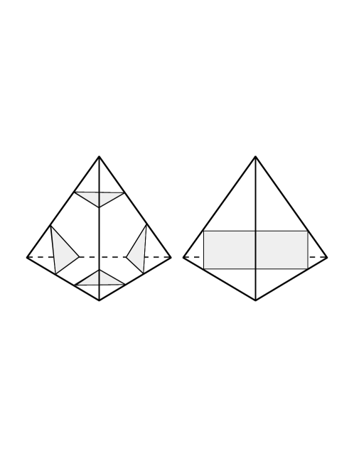
Figure 1: Normal triangles and normal quadrilaterals.

All four types of normal triangle can coexist disjointly in a 3-simplex. However as soon as one normal quadrilateral is around, the other two types of normal quadrilateral can not be present, or else an intersection would occur.

Definitions: A compressing disk for a surface $F$ inside a 3-manifold $M$ is an embedded disk in $M$ which meets $F$ along its boundary. We call the compressing disk non-trivial if the boundary curve of the disk does not bound a disk on $F$. A surface with no non-trivial compressing disks is incompressible. A boundary compressing disk for a surface with boundary $F$ is an embedded disk in $M$ with an arc of its boundary on $F$ and the remainder of its boundary on $\partial M$. We call the boundary compressing disk non-trivial if the arc on $F$ is not parallel to the boundary of $F$. A surface with no non-trivial boundary compressing disks is boundary incompressible. A non-trivial compressing disk can be used to squeeze off a handle of a surface, a process called compression, as in Figure 2. A similar process called boundary compression squeezes arcs on a surface into the boundary of a 3-manifold, as in Figure 3.

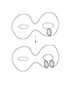
Figure 2: A compressing disk for a surface and the result of a compression.

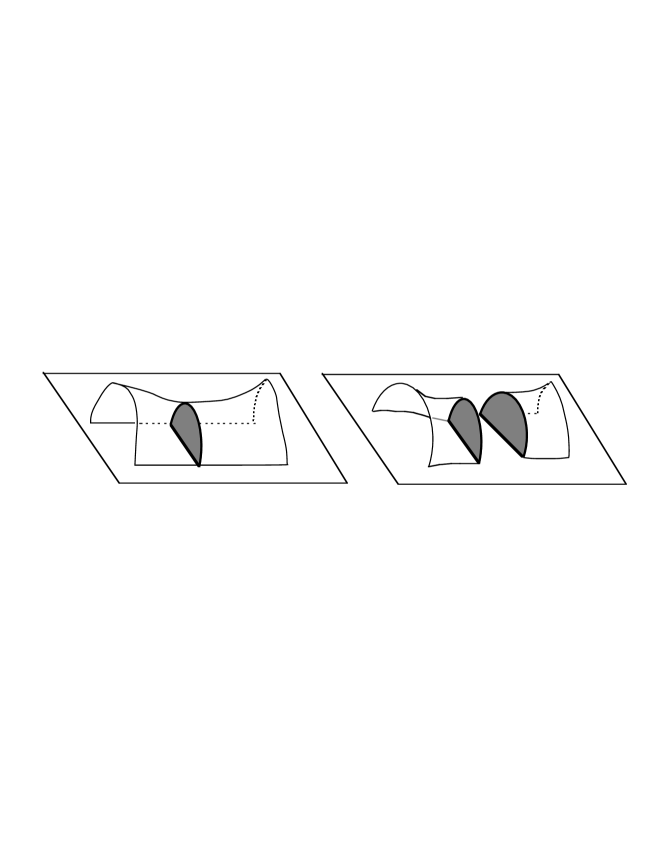
Figure 3: A boundary compressing disk for a surface and the result of a boundary compression.

4 Kneser’s Theorem

A 3-manifold $M$ which contains a separating 2-sphere can be cut open into two 3-manifolds with 2-sphere boundaries. By gluing in 3-balls to the boundaries, we get two new closed 3-manifolds $M_{1}$ and $M_{2}$. We say that the original manifold is the connect sum of these two manifolds, $M=M_{1}\#M_{2}$, which are called the summands. This operation is well defined and associative if each manifold is oriented and the gluing map of the two 2-spheres is required to reverse orientation. If the 2-sphere bounds a ball, then one summand is homeomorphic to $M$ and the other to the 3-sphere. This decomposition is called trivial. The question arises whether it’s possible to keep on splitting $M$ indefinitely in a non-trivial way, into more and more pieces.

Normal surfaces were introduced by Kneser, who used them to prove the following result [13].

Theorem 1

Let $M$ be a triangulated 3-manifold with $t$ 3-simplices and let $k(M)=\mbox{dim}(H_{1}(M;Z_{2}))+\mbox{dim}(H_{1}(M;Z))+6t$. Them $M$ can be decomposed non-trivially along 2-spheres into at most $k(M)$ pieces.

Suppose we have a collection of disjoint embedded 2-spheres in $M$. We will put the 2-spheres in a rigid position, making each of them a special type of surface.

In fact we will show that any embedded surface, not necessarily connected, can be compressed and isotoped to a union (possibly empty) of normal surfaces. To do so we introduce a notion of how complex a surface is relative to a given triangulation. The weight $w(F)$ of a surface $F$ is the number of times it intersects the 1-skeleton of $M$. Weight gives an analog of area in the PL context. It equals the area in the limiting case when all area measure is concentrated near the 1-skeleton.

Lemma 2

Let $F$ be an embedded surface in $M$. Then after a series of compressions, isotopies and removal of trivial 2-spheres, $F$ becomes isotopic to a union (possibly empty) of disjoint normal surfaces.

Proof: Consider the intersection of $F$ with the triangulation. After a slight perturbation of $F$, we can assume this intersection is transverse. We will simplify the intersection by a process which we call normalization.

$F$ intersects the interior of a tetrahedron $T$ in a collection of subsurfaces $F\cap T$, with boundary a collection of disjoint simple closed curves. The boundary of $T$ is a 2-sphere, and each simple closed curve in $F\cap\partial T$ cuts $\partial T$ into two disks. By applying the Loop Theorem of Papakyriakopoulous [19] [6], we can find a series of compressions in $T$ which yield a new surface, all of whose components meet $T$ in disks and 2-spheres. Since $T$ is a ball, and therefore irreducible, the 2-sphere components are trivial and can be discarded. The weight does not increase in this process, though the number of components of $F$ may rise. Repeating for each tetrahedra, we arrive at a surface $F_{1}$ of no higher weight with every curve in $F_{1}\cap\partial T$ bounding a disk in $T$.

If a curve in $F_{1}\cap\partial T$ lies completely inside a face of $T$, then we can isotop the disk it bounds in $T$ across that face and eliminate the curve, as well as any curves that lie inside it on the face. Repeating for other tetrahedra, we can assume that no such curves exist in a face of any tetrahedron.

Now suppose that there is a curve $\delta$ of $F_{1}\cap\partial T$ that meets an edge of $T$ in more than one point. If we consider all points of intersection of that edge with $F_{1}$, we can find an adjacent pair of points which lies on one curve of $F_{1}\cap\partial T$. These points can be connected by an arc on $F_{1}\cap T$ whose interior is in the interior of $T$. We can isotop this arc on $F_{1}$ across the edge segment between these two points, reducing the weight of $F_{1}$ by two.

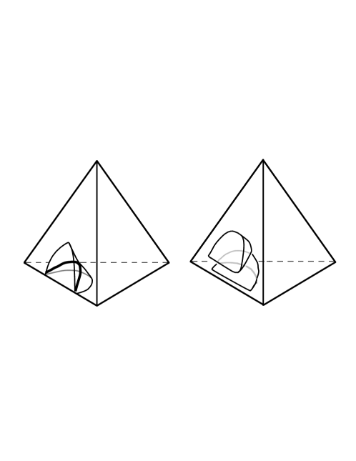
Figure 4: An isotopy across an edge of a tetrahedron reduces weight.

Repeating in all the tetrahedra, we arrive at a surface whose curves of intersection with the boundary of any tetrahedron meet each edge at most once. A disk in a tetrahedron whose boundary meets each edge at most once can only be a normal triangle or quadrilateral. The resulting surface is a disjoint union of normal surfaces and surfaces completely contained in a single tetrahedron. These latter surfaces can be compressed to give trivial 2-spheres by an application of the Loop Theorem, and the trivial 2-spheres can then be removed, leaving a normal surface as claimed.

To illustrate the close connection between normal surfaces and minimal surfaces, we now state an important theorem of W. Meeks, L. Simon and S.T. Yau [18]. Lemma 2 is essentially the same theorem in the PL context.

Theorem 3

Let $F$ be an embedded surface in a Riemannian 3-manifold $M$. Then after a series of compressions, isotopies, and collapsing of the boundary of an I-bundle to its core, $F$ can be realized as a union (possibly empty) of disjoint embedded minimal surfaces.

The extra process of collapsing I-bundles can be seen in the Mobius band, where a shortest curve isotopic to the boundary can be homotoped to double cover the core. In the Riemannian setting, the metric may force the minimizer to be a double cover. In the PL setting, this type of collapse is not necessary, even where it is possible.

Each 3-simplex contains four distinct types of normal triangle and three types of quadrilaterals. A good way to keep track of them is to notice that each normal triangle cuts off a unique vertex, and each normal quadrilateral separates one opposite pair of edges of the 3-simplex. In a given 3-simplex, a union of normal triangles and quadrilaterals can contain at most five types, - up to four triangles and at most one quadrilateral. Of course many parallel copies of one of the disk types can occur without causing intersections. The complementary regions in the 3-simplex consist of a collection of product regions, {triangle}$\times$I or {quadrilateral}$\times$I, together with at most six exceptional regions, which are not products. The exceptional regions meet either a vertex or at least two distinct disk types. The two tetrahedra in Figure 1 contain five and two exceptional regions respectively.

Proof of Kneser’s Theorem: Let $\{S_{1},S_{2},\dots,S_{n}\}$ be disjoint 2-spheres in $M$, no subset of which bounds a ball with some open balls removed, which we call a punctured ball. Let $F$ denote their union, and apply Lemma 2 to $F$. Then we can isotope and compress to obtain a normal surface. A compression causes a 2-sphere $S$ to be split into two 2-spheres $S_{1}$ and $S_{2}$. The property that no subset of the set of spheres bounds a ball may not be preserved after the compression. However if $S_{1}$ together with some other spheres bounds a punctured ball $B_{1}$, and $S_{2}$ together with some other spheres bounds a punctured ball $B_{2}$, then $S$ together with some other spheres also bounds a punctured ball. So we can replace $S$ by one of $S_{1}$ and $S_{2}$ and get a new set of spheres still having the property that no subset bounds a punctured ball. Repeating, we arrive at a collection of normal 2-spheres with this property which is as large as the initial collection.

We now show that if there are more than $k(M)$ disjoint normal 2-spheres, then a subset bounds a punctured ball, which implies there is a trivial $S^{3}$ summand in the decomposition they define. Each tetrahedron contains at most 6 non-product regions. The number of components of $M-F$ which are not built entirely out of product regions is bounded by $6t$. The product region components of $M-F$ are $I$-bundles with boundary a 2-sphere, and are either homeomorphic to $S^{2}\times I$ or to a non-trivial $I$-bundle over an embedded projective plane in $M$. Each of the latter components contributes an $RP^{3}$ to the connect sum decomposition of $M$, and a generator to $H_{1}(M;Z_{2})$. So the number of components of the complement of the collection of 2-spheres is bounded by $H_{1}(M;Z_{2})+6t$. This gives a bound to the number of separating 2-spheres in our collection. The number of non-parallel disjoint non-separating 2-spheres is bounded by $H_{1}(M;Z)$. So if the number of 2-spheres is greater than $k(M)$ then some subset of them must bound a punctured ball.

Kneser’s Theorem led to the establishment by Milnor of a unique factorization theorem for 3-manifolds into prime pieces. See [6] for an exposition.

An almost identical argument proves a theorem of Haken [3].

Theorem 4

Let $M$ be a triangulated 3-manifold with $t$ 3-simplices and let $k(M)=\textstyle{dim}(H_{1}(M;Z_{2}))+\textstyle{dim}(H_{1}(M;Z))+6t$. Then $M$ contains at most $k(M)$ disjoint, non-parallel, incompressible surfaces.

5 Recognizing the unknot.

Haken realized that the theory of normal surfaces had powerful applications in the study of 3-manifolds. He used them in two important ways.

1. To establish finiteness results about the number of ways in which manifolds can be cut open along surfaces other than 2-spheres. Haken showed that cutting manifolds open along suitably chosen incompressible surfaces resulted in a process which terminated after a finite number of steps [3]. Incompressible surfaces have assumed a central role in the theory of 3-manifolds. The 3-manifolds which are irreducible and which contain incompressible surfaces are called Haken manifolds.

2. To give algorithms to solve problems in 3-dimensional topology.

We will concentrate on the second contribution, and describe Haken’s algorithm to recognize the unknot among the knots in the 3-sphere [2].

A knot is the unknot if it bounds an embedded disk in $S^{3}$. The algorithm will search for this disk, and either produce it or show it does not exist in a finite amount of time. In fact, the same algorithm can find an embedded surface of smallest genus whose boundary is the knot, giving the genus of the know. The knot is the unknot if and only if this smallest genus surface is a disk. The surface will be described as a normal surface.

To allow this, we need to extend the notion of normal surface to surfaces and 3-manifolds with boundary. The definitions and pictures are the same, except that some faces of some tetrahedra lie on the boundary of the 3-manifold, giving a triangulation of the boundary. Lemma 2 generalizes with the extra operation of boundary compression.

To get started, we need to describe a 3-manifold and a surface with a finite amount of data. A 3-manifold is described nicely by a triangulation. The data is a finite set of vertices, and finite sets of pairs, triples and quadruples of vertices representing edges, faces and 3-simplices. There are some obvious conditions, such as that the three pairs constructed from a triple of vertices representing a face must occur as edges. We allow these sets of vertices to contain a vertex or edge more than once, since our 3-simplices are not required to be combinatorial.

Describing a surface will need some additional data. Taking advantage of Lemma 2, we work with normal surfaces. For each tetrahedron we have seven types of normal triangles and quadrilaterals. Assign to the $7t$ disk types found in the 3-manifold the labels $\{\sigma_{i}\}$ and let $x_{i}$ denote the multiplicity with which the disk type $\sigma_{i}$ occurs, $\ 1\leq i\leq 7t$. The vector of non-negative integers $x_{i}$ completely determines any embedded normal surface.

We now ask which non-negative integer vectors $x_{i}$ give rise to a normal surface. Two conditions must be met.

1. Each tetrahedron contains at most one type of quadrilateral. This is called the quadrilateral condition.

2. The disks must match up across a face separating two tetrahedra.

The first condition means that if certain $\sigma_{i}$ have non-zero coefficients, then others must have zero coefficients. The second means that the number of quadrilaterals and triangles in a tetrahedron having a given arc of intersection with a particular triangular face must equal the corresponding sum in the tetrahedron adjacent across that face. Since each arc on a triangular face of a tetrahedron can be part of the boundary of exactly one type of normal triangle and one type of normal quadrilateral, this leads to equations of the form $x_{i_{1}}+x_{i_{2}}=x_{i_{3}}+x_{i_{4}}.$ These linear equations are called the matching equations. There are three of them for each pair of tetrahedral faces which are glued to one another. Together with the conditions $0\leq x_{i}$ we call them the normal surface equations. There are no matching equations associated to boundary faces. Solutions of the normal surface equations can have boundaries contained in these faces. If the quadrilateral condition and the normal surface equations hold, then the integers $x_{i}$ give a unique embedded normal surface, constructed by gluing together the normal triangles and quadrilaterals in the unique way giving an embedding. We denote by $X$ the vector of non-negative integers $(x_{1},x_{2}\ldots,x_{n})$, and also use $X$ to denote the embedded normal surface made from the union of $x_{i}$ copies of the normal piece $\sigma_{i}$.

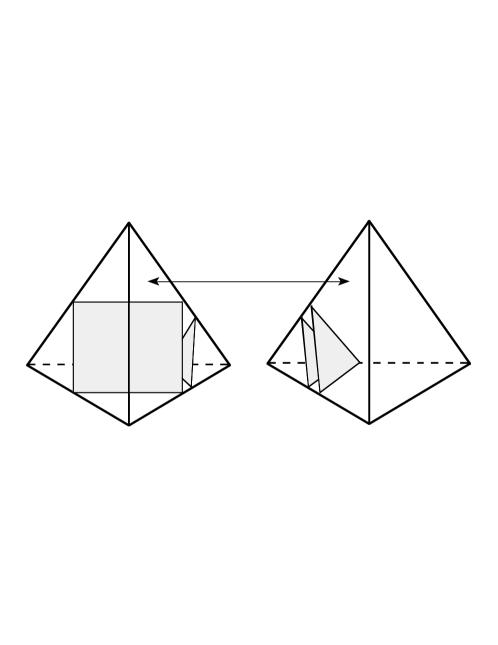
Figure 5: Elementary disks in adjacent tetrahedra match up.

Two normal surfaces $A$ and $B$ may intersect one another. A surface $C$ is obtained by taking their union and doing an operation called regular exchange. This involves cutting and pasting along double curves so as to preserve the property that all disks are normal. There is always a unique way to cut and paste two normal disks intersecting along an arc to obtain a pair of disjoint normal disks, unless they are non-parallel quadrilaterals. In that case no choice will give normal disks.

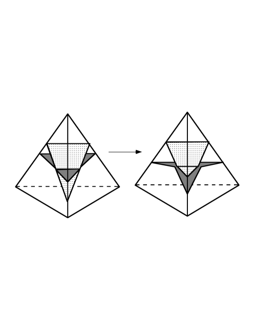
Figure 6: A regular exchange keeps all disks normal.

Lemma 5

If $A,B,C$ are solutions of the normal surface equations with $A+B=C$, and $C$ gives rise to an embedded normal surface, then so do $A$ and $B$. Furthermore, $\chi(C)=\chi(A)+\chi(B)$ and $w(C)=w(A)+w(B)$.

Proof: If $C$ corresponds to an embedded surface then it satisfies the quadrilateral condition, so it doesn’t contain intersecting quadrilaterals, and neither do $A$ or $B$. We can calculate the Euler characteristic of $C$ by counting vertices, edges and faces. The same number of each form $C$ and $A\cup B$. The weight is unchanged when regular exchanges are made, and $C$ is obtained from $A\cup B$ by making regular exchanges.

A solution $C$ of the normal surface equations is fundamental if it cannot be written as a sum of two other solutions, $C\neq A+B$.

Lemma 6

The set of fundamental solutions to the normal surface equations is finite.

Proof: Real non-negative solution to the normal surface equations form a cone contained in $R_{+}^{n}$. We can intersect this cone with the convex simplex defined by $\Sigma x_{i}=1,x_{i}\geq 0$ and obtain a convex polyhedron with finitely many vertices $v_{j}$. The non-negative integer solutions are rational multiples of points in this polyhedron. Thus any solution of the normal surface equations can be expressed as a rational linear combination of the vertex solutions $v_{j}$. Consider now integral multiples $V_{j}=\lambda_{j}v_{j}$ of the $v_{j}$. The normal surfaces $V_{j}$ also form a rational basis for all normal surfaces, so any normal surface $X$ can be expressed in the form $X=\Sigma t_{j}V_{j}$ with $0\leq t_{j}$. Now consider the set $S$ of real solutions to the normal surface equations which can be expressed in the form $s=\Sigma t_{j}V_{j}$ with $0\leq t_{j}\leq 1,1\leq j\leq n$. $S$ is compact, and so contains a finite number of integral points. If $X$ is an integral solution of the normal surface equations not in $S$, then some $t_{k}>1$ and we can write $X$ as the sum of two other positive integral solutions, $X=V_{k}+(\Sigma t_{j}V_{j}-V_{k})$. Thus all fundamental solutions lie in $S$, and there are only finitely many.

Some subset of these fundamental solutions, those that also satisfy the quadrilateral condition, correspond to embedded surfaces.

The following result is due to Schubert [23].

Lemma 7

If $C$ is a connected normal surface in an irreducible 3-manifold and $C$ is not fundamental then we can find connected normal surfaces $A$ and $B$ so that $C=A+B$. If $A$ and $B$ are chosen to minimize the number of curves of intersection in $A\cap B$, then no curve in $A\cap B$ is separating in both $A$ and $B$.

Proof: Suppose $C=A_{1}+A_{2}\ldots+A_{k}$, where each $A_{i}$ is an embedded normal surface. If $A_{2}$ intersects $A_{1}$, then we can perform regular exchanges successively along each curve in their intersection. The number of surfaces adding to $C$ changes by at most one each time we perform a regular exchange. Continuing for each surface $A_{j}$, we eventually arrive at a connected surface $C$, so at some point we must get two connected surfaces whose sum is $C$. If these are not embedded, we can perform regular exchanges along their curves of self-intersection, giving a possibly larger collection of embedded surfaces. There are only finitely many curves on which we can do a regular exchange so the process stops with two embedded surfaces whose sum is $C$.

Now pick $A$ and $B$ to minimize the number of curves of intersection in $A\cap B$ among all pairs of connected embedded normal surfaces whose sum gives $C$. Suppose a curve $\alpha$ in $A\cap B$ separates in both $A$ and $B$. Then a regular exchange along $\alpha$ cannot result in a single connected surface. It must result in two connected surfaces $A^{\prime}$ and $B^{\prime}$, possibly non-embedded. Regular exchanges on all self-intersection curves of $A^{\prime}$ and $B^{\prime}$ results in embedded surfaces $A^{\prime\prime}$ and $B^{\prime\prime}$, possibly not connected, whose sum is $C$. If $A^{\prime}$ and $B^{\prime}$ are not connected, then we can carry out a series of regular exchanges until we again arrive at exactly two connected surfaces. Eventually we obtain $C$ as a sum of two embedded surfaces with fewer curves of intersection than $A$ and $B$, a contradiction.

A curve on the boundary torus of a knot complement is essential if it does not bound a disk on the torus. The following lemma allows us to reduce the search for an unknotting disk to the finite collection of fundamental surfaces. Our proof is based on that of Jaco-Oertel[9].

Lemma 8

Suppose $C$ is a normal disk in a knot complement, with minimal weight among all normal disks with essential boundary. Then $C$ is fundamental.

Proof: If the lemma fails, then we can find two connected normal surfaces $A$ and $B$ such that $C=A+B$. Pick $A$ and $B$ as in Lemma 7. Since $\chi(C)=1=\chi(A)+\chi(B)$, we have several possibilities. 1. $A$ is a punctured torus and $B$ a 2-sphere. 2. $A$ is a punctured Klein-bottle and $B$ a 2-sphere. 3. $A$ is a disk and $B$ a torus. 4. $A$ is a disk and $B$ an annulus. 5. $A$ is a disk and $B$ a Mobius band. Possibilities involving embedded Klein bottles and projective planes, though not more difficult, cannot occur in a knot complement.

In each case we can obtain a contradiction. An argument used in [9] for closed surfaces, extends to our setting. This extension is explicitly derived in [11]. In each of the above cases, if $C=A+B$ then we can find $A^{\prime}$ and $B^{\prime}$ such that $C=A^{\prime}+B^{\prime}$ where $A^{\prime}$ is an essential disk and $B^{\prime}$ is a torus or an annulus. The essential normal disk $A^{\prime}$ has lower weight than $C$, a contradiction.

Note: An alternate way to obtain a contradiction can be found by taking $C$ to be of minimal complexity, as measured in the sense of Jaco-Rubinstein [10]. In this setting the complexity measures the length of intersection of a normal surface with the 2-skeleton of a triangulation.

Theorem 9

There is an algorithm to decide whether a knot is the unknot.

Proof: Triangulate the knot complement $M_{K}$ and construct the finitely many fundamental solutions. Among them find the ones satisfying the quadrilateral conditions. By calculating the Euler characteristics, check if any of these are disks. If yes, test if the boundary of the disk is essential on $\partial M_{K}$ by checking whether it disconnects $\partial M_{K}$. If there is a disk with essential boundary on $\partial M_{K}$ then $K$ is the unknot. If there is no such disk it is not.

We now show why the algorithm works. Suppose $K$ is the unknot. Then it bounds a disk. Lemma 2 implies that there is a normal disk $D$ which bounds an essential curve on $\partial M_{K}$. Lemma 8 implies we can find such a disk among the fundamental solutions. So the algorithm finds an unknotting disk if it exists.

6 Other algorithms to recognize the unknot.

One might hope that an approach involving a search for moves that simplify a knot projection would give an algorithm to recognize the unknot. No approach using this idea has been found. The following projection of the unknot, suggested by Cameron Gordon, shows that if one wants to use a sequence of Reidemeister moves, it may be necessary to increase the number of crossings on the way to the unknot. It is an interesting open problem to find a larger class of allowable moves which would allow monotonic progress towards the unknot.

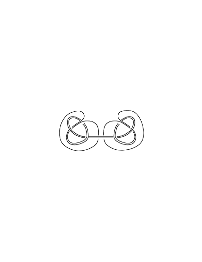
Figure 7: The number of crossings in this projection of the unknot must be increased before it can be decreased using Reidemeister moves.

Alternate algorithms to recognize the unknot could follow from a better understanding of certain knot invariants. It is conjectured that the Jones polynomial of a knot equals 1 if and only if the knot is the unknot. Since there is a simple finite procedure for computing the Jones polynomial of a knot, a proof of this conjecture would provide an algorithm to decide if a knot is the unknot.

Kuperberg has pointed out that Thurston’s work on geometric structures on 3-manifolds gives an alternate approach to constructing knot triviality algorithms, one of which we now describe. We will refer to it as an algebraic algorithm.

This algorithm considers PL knots, as before. We triangulate the 3-sphere and consider a knot contained in the 1-skeleton. The algorithm tests whether this knot is the unknot by running two processes in parallel.

The first process checks if the knot is unknotted by looking for embedded disks in the 2-skeleton. If it fails to find any, it takes a barycentric subdivision and repeats. The process ends if it finds a disk, in which case the knot is unknotted.

The second process searches for a non-cyclic finite representation of the fundamental group of the knot, in the following way. It first computes the Wirtinger presentation of the fundamental group of the knot complement. It then computes all homomorphisms of the group to the groups $S_{3},S_{4},S_{5}\ldots$, where $S_{n}$ is the group of permutations of $n$ elements. All homomorphisms to $S_{n}$ can be constructed by mapping the Wirtinger presentation generators to the finitely many possible sets of elements in $S_{n}$, and checking whether the relations of the knot group are satisfied in $S_{n}$. The process stops if it finds a homomorphism with non-cyclic image, in which case it concludes that the knot is non-trivial.

Theorem 10

The algebraic algorithm described above gives an algorithm to decide whether a knot is the unknot.

Proof: If the knot is unknotted, the first process will end after a finite amount of time.

If the knot is not the unknot, then it is a consequence of the existence of geometric structures on knot complements that the fundamental group of the knot complement is a non-abelian residually finite group [7]. Residually finite means that for any non-trivial element of the group, there is a homomorphism to some finite group which takes that element to a non-trivial element of the finite group. There is no loss of generality in considering as images only the groups $S_{n}$, which contain all other finite groups as subgroups.

A non-abelian residually finite group has a non-trivial commutator subgroup. An element of this subgroup has non-trivial image in some $S_{n}$ under some homomorphism. If the image of all homomorphisms of the group were cyclic, and therefore abelian, then this element would always map to the trivial element, contradicting residual finiteness. So for some element and some $S_{n}$ the image of the group is non-cyclic.

The process is guaranteed to stop after a finite time in either case.

7 Classifying knots.

To classify all knots we need to be able to decide not just whether a knot is the unknot, but whether two arbitrary knots $K_{1}$ and $K_{2}$ are the same. This was carried out by Haken and Hemion using some additional arguments based on normal surfaces [5]. We outline very briefly here an extension of the algebraic algorithm described above that can also give such a classification. This emerges from work of Thurston, and was also related to me by Kuperberg. We call it the geometric algorithm to distinguish knots.

Assume we are given two knots, $K_{1}$ and $K_{2}$, each presented as an embedded circle in the 1-skeleton of a triangulation of the 3-sphere. The idea is to set two processes in motion, one of which will terminate if the knots are the same, the other if they are different. Call the two triangulations $T_{1}$ and $T_{2}$. The first process checks if $T_{1}$ is equal to $T_{2}$ by an isomorphism carrying $K_{1}$ to $K_{2}$. If not, it performs a bistellar move on $T_{1}$ and checks again. After trying all bistellar moves on $T_{1}$, it performs all pairs of bistellar moves. Eventually it will get to all sequences of $k$ successive bistellar moves. If the two knots are the same, this will terminate in finite time.

The second process will terminate in finite time if the knots are distinct. It has two stages, first constructing geometric structures on each knot complement, and then checking if they are distinct. It generates a series of subprocesses, run in parallel, as it tries different triangulations. It searches for the geometric structures on each knot complement, which must exist by Thurston’s geometrization theorem. The geometric structure is constructed by triangulating the complement, with the tetrahedra allowed to be ideal, and constructing geometric structures on each tetrahedron so that the angles at edges and vertices match up. If no compatible collection of angles can be constructed, then the process looks for tori and annuli in the 2-skeleton along which to cut up the knot complement, and tries to geometrize each piece. If it fails, it subdivides barycentrically and repeats. After a finite amount of time, geometric structures on each knot complement will be found by this process. Moreover the meridian of the knot and the gluing maps along splitting tori can be marked and remembered. It remains to check if these structures determine distinct knots. This can be done by putting an $\epsilon$ net on one 3-manifold, and trying to construct an isometry of this net into the second knot complement, preserving markings. If this is impossible, then the knots are distinct. If possible, then the process picks $\epsilon$ smaller and tries again. If the knots are distinct, the process will fail to construct an isometry eventually, and so will terminate in finite time, establishing that the knots are different.

8 Other recognition results.

In this section we briefly describe some other results on the problem of recognizing knots and three dimensional manifolds.

Schubert developed an alternate view of normal surfaces based on handle theory. He gave an algorithm to decide if a link is split [23]. This approach is also used in Jaco and Oertel [9], where an algorithm to decide if a 3-manifold is Haken is developed. Haken and Hemion solved the recognition problem for Haken manifolds [5]. Rubinstein extended the notion of normal surfaces to the concept of almost normal surfaces. He used this to describe an algorithm which decides whether a 3-manifold is homeomorphic to the 3-sphere [22]. Thompson gave an elegant argument that this algorithm works by using the notion of thin position [26]. Rubinstein also described algorithms to recognize Lens spaces and other 3-manifolds of small genus. See also Stocking [25]. Rubinstein and Rannard have recently announced an algorithm to recognize Seifert Fibered manifolds. Sela gave an algorithm to decide whether two 3-manifolds with Gromov hyperbolic fundamental group are homotopy equivalent [24]. Birman and Hirsch [1] have recently announced a new algorithm, based on work of Birman and Menasco, which detects whether a knot presented in braid form is the trivial knot. Jaco and Tollefson describe algorithms to construct maximal families of 2-spheres in a 3-manifold in [11]. They also develop the important idea of a vertex surface, a type of fundamental normal surface introduced by Jaco and Oertel in [9], which gives a more specialized representative for a class of surfaces. In [4] a bound for the complexity of the unknotting algorithm is given. It is also shown that this problem is in the class NP. Casson has recently announced a computation of the compexity of th 3-sphere recognition algorithm, which shows that it is also in the class NP.

References

- [1] J. Birman and M. Hirsch, Recognizing the Unknot, preprint.
- [2] W. Haken, Theorie der Normalflachen, Acta. Math. Vol. 105, 1961, 245-375. 1961, 245-375.
- [3] W. Haken, Connections between topological and group theoretical decision problems, Word Problems, W.W. Boone (Ed.) North Holland, Amsterdam 1973, 427-441.
- [4] J. Hass, J. Lagarias and N. Pippenger, The computational complexity of knot and link problems, preliminary report, Proc. 38th Annual Symposium on Foundations of Computer Science, 1997, 172-1181.
- [5] G. Hemion, The Classification of Knots and 3-dimensional Spaces, Oxford University Press, 1992.
- [6] J. Hempel, 3-manifolds, Annals of Math Studies 86, Princeton U. Press 1976.
- [7] J. Hempel, Residual finiteness for 3-manifolds, Combinatorial group theory and topology, Alta, Utah, 1984, Ann. of Math. Stud., 111, Princeton, 379-396. Univ. Press, Princeton, NJ, 1987.
- [8] J. Hopcroft and J. Ullman, Introduction to automata theory, languages and computation, Addison Wesley 1979.
- [9] Jaco, W. and Oertel, U., An Algorithm to Decide if a 3-Manifold is a Haken Manifold, Topology Vol. 23, No. 2, 1984, pp. 195-209.
- [10] W. Jaco and J.H. Rubinstein, A piecewise linear theory of minimal surfaces in 3-manifolds, J. Diff. Geom. Vol. 27, (1988), 493-524.
- [11] W. Jaco and J.L. Tollefson, Algorithms for the complete decomposition of a closed -manifold, Illinois J. Math. 39 (1995), 358-406.
- [12] K. Johannson, Classification problems in low-dimensional topology, Geometric and algebraic topology, Banach Center Publ., 18, PWN, Warsaw (1986) 37-59.
- [13] H. Kneser, Geschlossene Flachen in dreidimesionalen Mannifgfaltigkeiten, Jahresericht der Ent. Math. Verein 28 (1929) 248-260..
- [14] S. V. Matveev, Algorithms for the recognition of the three-dimensional sphere (after A. Thompson). Mat. Sb. 186 (1995) 69-84.
- [15] A.A. Markov, Insolubility of a problem of homeomorphy, Proc. International Congress of Mathematicians (1958) Cambridge Univ. Press, 300-306.
- [16] E.E. Moise, Affine Structures in 3-manifolds V, Annals of Math. 55 (1952) 96-114.
- [17] W. H. Meeks and S.T.Yau, Topology of three dimensional manifolds and the embedding theorems in minimal surface theory, Annals of Math. 112 (1980) 441-484.
- [18] W. Meeks, L. Simon and S.T. Yau, Embedded minimal surfaces, exotic spheres and manifolds of positive Ricci curvature, Annals of Math. 116 (1982) 621-659.
- [19] C.D. Papakyriakopoulous, On Dehn’s lemma and the asphericity of knots, Annals of Math. 66 (1957), 1-26.
- [20] J. J. Rotman, The Theory of Groups, Second Ed., Allyn and Bacon (1973).
- [21] J.H. Rubinstein, Polyhedral minimal surfaces, Heegaard splittings and decision problems for 3-dimensional manifolds, Proceedings of the Georgia Topology Conference, (1993) AMS/Intl. Press, 1-20.
- [22] J.H. Rubinstein, An algorithm to recognize the 3-sphere, to appear in Proceedings of the ICM, Zurich 1994. 3.
- [23] H. Schubert, Bestimmung der Primfaktorzerlegung von Verkettungen, Math. Z. 76 (1961) 116-148.
- [24] Z. Sela, The isomorphism problem for hyperbolic groups I. Annals of Math. 141 (1995) 217-283.
- [25] M. Stocking, Almost normal surfaces in 3-manifolds. Ph.D. Thesis, UC Davis (1996).
- [26] A. Thompson, Thin Position and the Recognition Problem for , Math. Research Letters 1, (1994) 613-630.
- [27] W. Thurston, The geometry and topology of 3-dimensional manifolds, Princeton University Lecture Notes (1978).
- [28] F. Waldhausen, Recent results on sufficiently large 3-manifolds, Proc. Sympos. in Pure Math. 32, Amer. Math. Soc. (1978) 21 - 38.
- [29] F. Waldhausen, Some problems on 3-manifolds, Proc. Sympos. in Pure Math. 32, Amer. Math. Soc. (1978) 313-322.
Joel Hass
Department of Mathematics
University of California
Davis, CA 95616
e-mail: hass@@math.ucdavis.edu